Histogram Methods for Quantum Systems: from
Reweighting to Wang-Landau Sampling
Matthias Troyer, Fabien Alet,
Theoretische Physik, ETH Z¨urich, CH-8093 Z¨urich, Switzerland
Computational Laboratory, ETH Z¨urich, CH-8092 Z¨urich, Switzerland
and Stefan Wessel
Theoretische Physik, ETH Z¨urich, CH-8093 Z¨urich, Switzerland
Received on 2 September, 2003
We discuss how reweighting and histogram methods for classical systems can be generalized to quantum models for discrete and continuous time world line simulations, and the stochastic series expansion (SSE) method. Our approach allows to apply all classical reweighting and histogram techniques for classical systems, as well as multicanonical or Wang-Landau sampling to the quantum case.
1
Introduction
Quantum Monte Carlo simulations have become almost as powerful as classical simulations, despite their usually more complex formulation and implementation.
Not only local update algorithms,[1] but also general-izations of the classical cluster Monte Carlo algorithms [2] have been developed for quantum systems, solving the prob-lem of critical slowing down at some important second order phase transitions.[3, 4, 5] Some cluster update algorithms, such as the worm algorithm [6] have even originally been developed for quantum models before being applied to clas-sical ones.[7]
Here we show that also classical reweighting, histogram sampling methods, and the Wang-Landau algorithm[8] can be adapted to quantum systems, expanding on technical is-sues omitted in Ref. [9]. Histogram reweighting [10] allows simulation results to be obtained in a range of temperatures (or couplings) from simulations performed at a single tem-perature. It is useful in accurately finding critical points, the Wang-Landau algorithm [8], which is related to multicanon-ical sampling [11] eases tunneling through free energy bar-riers at first order phase transitions.
We start with a short review of the classical histogram reweighting before discussing how it can be generalized to quantum systems, and finish with applications of a quantum version of Wang-Landau sampling.
2
Classical Monte Carlo simulations
2.1
Histogram reweighting
In a classsical system the thermal average of a quantityAat an inverse termperatureβis defined as a sum over all
con-figurations
A(β)= 1
Z
c
Ace−βEc, (1)
whereAc is the measurement of the observable A in the
configurationcandEc the energy of that configuration. In
a Monte Carlo simulations, a subset ofM configurations {ci}, drawn with probabilitypc = exp(−βEc)is sampled,
and the thermal average estimated by the sample mean
A(β) ≈A= 1
M
i
Aci. (2)
This sampling scheme gives results only for the inverse temperatureβ, but actually there is much more information available than just the simple average Eq. (2). Indeed, in the search for a phase transition a range of temperatures needs to be explored and information at a nearby inverse temper-atureβ′ ≈βcan be obtained from a simulation performed atβ. This is done by reweighting the configurations sam-pled with the Boltzmann weightpc= exp(−βEc)to obtain
averages for the Boltzmann weightp′
c= exp(−β′Ec):
A(β′) ≈
iAcip
′
ci/pci
ip′ci/pci
(3)
=
iAcie
−∆βEci
ie−∆βEci
(4)
where∆β =β′−β.
Instead of storing the full time series of measurements {Aci}and energies{Eci}, we now store a histogramH(E),
counting how often the energy levelEoccurs in the time se-ries{Eci}, and the averageA(E)of all the measurements
A(E) = 1
H(E)
iwithEci=E
Aci (5)
With these two histograms the averageA(β′)can be cal-culated as a sum over all energies
A(β′) ≈
EH(E)A(E)e−∆βE
EH(E)e−∆βE
(6)
Histogram reweighting works well only if the configu-rations sampled at the inverse temperatureβ are also rele-vant atβ′, requiring that∆β is small. Otherwise the errors become too large since there will not be sufficient entries inH(E)for the energiesE important atβ′. Multiple his-tograms obtained at different temperatures can be used to broaden the accessible temperature range.[10]
2.2
Wang-Landau sampling
While cluster updates, optionally combined with histogram reweighting, are an efficient solution to the problem of crit-ical slowing down at a second order phase transition they do not address the problem of tunneling between local free energy minima at a first order phase transition. There, the multicanonical algorithm[11] or Wang-Landau sampling can help.[8]
The key idea of the multicanonical method and Wang-Landau sampling is to calculate the density of statesρ(E)
directly by a random walk in energy space instead of per-forming a canonical simulation at a fixed temperature. If, instead of the Boltzmann weightp(E) ∝ exp(−βE) one uses the inverse density of statesp(E)∝1/ρ(E), the prob-ability of encountering a state with energyEchanges from
PBoltzmann(E)∝ρ(E)p(E) =ρ(E)e−βE (7) to a constant probability
PWang−Landau(E)∝ρ(E)
1
ρ(E) = const (8)
This algorithm should be much more efficient and solve the exponential tunneling problem, since one now performs a perfect random walk in energy space with a flat histogram. Naively one expects the scaling to be theO(N2)scaling of a random walk overN energy levels. In a detailed scaling analysis[12] we found that due to memory effects this is not a Markovian random walk. The scaling is slightly worse, but remains polynomial, for homogeneous non-frustrated and frustrated systems, and becomes exponential only for spin glasses.
Besides solving the tunneling problem at first order phase transitions, the Wang-Landau algorithm calculates the density of statesρ(E)in an iterative procedure. Knowledge ofρ(E)then allows the direct calculation of the free energy from the partition function
Z=
E
ρ(E)e−E/kBT
. (9)
The internal energy, entropy, specific heat and other thermal properties are easily obtained as well, by differentiating the free energy.
3
Quantum Monte Carlo
3.1
Generalizing histogram reweighting and
Wang-Landau sampling
Since simulations of quantum systems suffer from the same problems as classical simulations, in particular from long tunneling times at first order phase transitions and the in-ability to calculate the free energy directly, an extension of this algorithm to quantum systems is highly desired. The generalization is not immediately obvious since the partition function of a quantum system
Z = Tre−βH (10)
cannot be cast in the form of Eq. (9) unless the complete spectrum of the Hamilton operatorHis known.
Instead of a representation like Eq. (9) we will aim for a generalized representation of the form
Z =
(n1,...,nd)
g(n1, . . . , nd)p(β, n1, . . . , nd). (11)
where the tuple(n1, . . . , nd)describes properties of the
con-figuration that are sampled,p(β, n1, . . . , nd)is the weight of
that configuration, and the histogramg(n1, . . . , nd)counts
how many configurations there are with the same properties
(n1, . . . , nd). In the classical simulations discussed above
we had one-dimensional histiograms d = 1, the desired property was the energyn1=E, the weight the Boltzmann weightp(β, E) = exp(−βE)and the histogramg(E)the density of states.
Both histogram reweighting and Wang-Landau sam-pling are straightforwardly generalized to a representation (11). E.g., to employ Wang-Landau sampling, the weight
p(β, n1, . . . , nd) of a configuration in standard sampling
should be replaced by 1/g(n1, . . . , nd) and the algorithm
will perform a random walk with a flat histogram in the space of the(n1, . . . , nd).
We will now describe how the mapping to Eq. (11) can be done for quantum systems in three different rep-resentations: in discrete[13] and continuous time[14, 4] path integrals and in the stochastic series expansion (SSE) representation.[15]
3.2
Discrete Time Path Integrals
The historically first approach to quantum Monte Carlo sim-ulations of lattice models was based on the Trotter-Suzuki decomposition, by splitting the Hamilton operator H into two or more termsH = N
i Hi so that the exponentials
of each of the termsexp(−βHi)are easy to calculate.
Al-though theHido not commute, the error in estimating the
exp(−ǫH)≈
i
exp(−ǫHi) +O(ǫ2) (12)
is small for small prefactorsǫ. Applying this approximation to the partition function we get Suzuki’s famous mapping, here shown for the simplest case of a chain with nearest neighbor interactions with two terms H1 collecting terms on even bonds andH2terms on odd bonds:
Z = Tr
e−βH
= Tre−∆τ(H1+H2)M
= Tr
e−∆τ H1
e−∆τ H2M
+ O(∆τ2) (13)
=
i1,...,i2M
i1|U1|i2i2|U2|i3 · · · i2M|U2|i1 + O(∆τ2),
where the time step is∆τ = β/M, the|ikeach are
com-plete orthonormal sets of basis states, and the transfer ma-trices areUi = exp(−∆τ Hi). The evaluation of the matrix
elementsi|U1|i′is straightforward since theHiare chosen
to be easily diagonalized.
To see how this can be mapped to Eq. (11) let us con-sider a spin-1/2 model with Hamilton operator
H =
i,j
JxySixSjx+S y iS
y
j +JzSizSjz
(14)
Since each of theHiis a sum of commuting bond terms, we
can focus on a single bond term:
H=
Jz/4 0 0 0
0 −Jz/4 Jxy/2 0
0 Jxy/2 −Jz/4 0
0 0 0 Jz/4
, (15)
the exponential of which is
U =e−∆τ H=
p1 0 0 0
0 p2 p3 0
0 p3 p2 0
0 0 0 p1
(16)
with
p1 = e−∆τ Jz/4
p2 = e+∆τ Jz/4cosh(∆τ Jxy/2) (17)
p3 = e+∆τ Jz/4sinh(−∆τ Jxy/2)
The product of matrix elements in Eq. (13) can be expressed as integer powers of these matrix elements:
Z =
c=(i1,...,i2M)
p1n1(c)p2n2(c)pn33(c) (18)
=
(n1,n2,n3)
g(n1, n2, n3)fd(β, n1, n2, n3) (19)
with
fd(β, n1, n2, n3) = e(−n1+n2+n3)βJz/4M ×
[cosh(βJxy/2M]n
2
× (20)
[sinh(−βJxy/2M)]n3.
Using a three-dimensional histogram instead of a one-dimensional one all classical reweighting approches, such as histogram reweighting, [10] multicanonical sampling,[11] and the Wang-Landau algorithm[8] can now be applied to a quantum system.
3.3
Continuous Time Path Integrals
Simulations in discrete imaginary time with finite time steps
∆τrequire extrapolations to continuous time∆τ→0from calculations performed at several discrete time steps∆τ. For models with a finite number of states per lattice site, the limit∆τ →0can already be taken in the construction of the algorithm and simulations can be performed directly in the continuous time limit∆τ →0. Following Ref. [14], the continuous time limit can be formulated through time-dependent perturbation theory in imaginary time:
⌋
Z = Tr exp(−βH) = Tr
exp(−βH0)T exp− β
0
dτ V(τ)
,
= Tr
exp(−βH0)
1− β
0
dτ V(τ)dτ+ (21)
1 2
β 0
dτ1 β
τ1
dτ2V(τ1)V(τ2) +...
,
where the symbolT denotes time-ordering of the exponen-tial. The HamiltonianH =H0+V is split into a diagonal termH0which in our example of a spin-1/2 model is
H0=Jz
i,j
Sz
iSjz (22)
and an offdiagonal perturbationV:
V =Jxy
i,j
SixSxj +S y iS
y
j (23)
The time-dependent perturbation in the interaction rep-resentation isV(τ) = exp(τ H0)V exp(−τ H0). In order to gain an expression in the form of Eq. (11) we insert sums over complete sets of basis states and make the β depen-dence explicit by redefiningτi →βτi:
Z =
i1
i1|e−τ1βH0|i1+
∞
n=1
(i1,...,in)
(−β)n
n!
1
0
dτ1· · · 1
0
dτn
i1|e−τ1βH0|i1i1|V|i2i2|e−(τ2−τ1)βH0|i2 · · · · · · in|V|i1i1|e−(1−τn)βH0|i1 (24) Making use of the observation that all matrix elements ofV
areJxy/2we end up with an expression
Z=
c=(i1)
e−βE(c)+
∞
n=1
c=(i1,...,in)
(−βJxy/2)n
n!
1
0
dτ1· · · 1
0
dτne−βE(c),
=
dE
n
g(E, n)fc(β, E, n) (25)
whereE(c)is the averaged diagonal energy of the configu-rationc= (i1, . . . , in):
E(c) = (τ1+(1−τn))i1|H0|i1+
n
j=2
(τj−τj−1)ij|H0|ij
(26) and for the special casen= 0
E(c) =i1|H0|i1. (27)
We end up with Eq. (25), which is of the desired form of Eq. (11) with a two-dimensional histogramg(E, n)of the diagonal energiesEand expansion ordersn, and a weight function
fc(E, n) =e−βE(−βJxy/2)
n
n! . (28)
At this point we need to address two technical issues before we are able to implement histogram reweighting or Wang-Landau sampling. The first is that the energyEis a continuous variable and we need to discretize it by introduc-ing narrow energy bins of finite width∆E. The second is
that the sum over order nruns to infinity and needs to be truncated at some upper limit Λ. This truncation restricts the validity of the histogram reweighting or Wang-Landau sampling to inverse temperaturesβ <O(Λ/N)whereNis the number of lattice sites. By choosingΛlarge enough we can still reach down to any desired temperature.
3.4
Stochastic Series Expansion
In going from discrete to continuous time we not only got rid of the time discretization error but also simplified the his-togram from a three-dimensional to a two-dimensional one. We can formally do this by setting H0 = 0 andV = H in the above continuous time representation, which will re-sult in a constant E = 0 but at the cost of now perturb-ing in the diagonal part of the Hamiltonian (theJz term)
which was previously treated exactly. After integrating out the time integrals we obtain the stochastic series expansion (SSE) representation:[15] We start by expressing the parti-tion funcparti-tion as a high temperature expansion
Z = Tre−βH=
∞
n=0
βn
n!Tr(−H)
n
= Z(0) +
∞
n=1
βn n!
(i1,...,in)
i1| −H|i2 · · · in| −H|ii
≡ ∞
n=0
g(n)fSSE(β, n) (29)
whereZ(0) =g(0)is just the number of states in the Hilbert space and the weight function is (assuming for simplicity a Heisenberg model withJxy=Jz=Jon a bipartite lattice)
fSSE(β, n) =(βJ/2)
n
n! . (30)
Then-th order series coefficientg(n)now plays the role of the density of states in the classical algorithm and we can apply histogram reweighting or Wang-Landau sampling.
4
Application examples
0.838 0.8385 0.839 0.8395 0.84 T (J)
0.61 0.615 0.62 0.625 0.63 0.635 0.64
U
L=32 L=48 L=64 L=96
Figure 1. The Binder cumulant ratioU of a 3D quantum Heisen-berg ferromagnet obtained from histogram reweighting of multiple histograms obtained in an SSE simulation.
0.4 0.8 1.2 1.6 2.0
T / J
0.0 0.2 0.4 0.6 0.8 1.0
S
(
π,π,π
) /
L
2−
η
0.0 1.0 2.0
T / J
0.0 0.5 1.0
C
/
L
3
L=12
L=8
L=6
L=4
L=16
Figure 2. Scaling plot of the staggered structure factor of a cu-bic antiferromagnet as a function of temperature, obtained from simulations at a fixed temperature for various lattice sizes. The inset shows the specific heat as a function of temperature. The
cut-offΛ = 500(L/4)3
restricts the accessible temperature range to
T 0.4J.
To demonstrate Wang-Landau sampling for quantum systems, we first consider a second order thermal phase transition in the Heisenberg antiferromagnet on a simple cubic lattice. From simulations of systems with L3 sites,
L = 4,6,8,12,16, we can calculate the staggered struc-ture factorS(π, π, π)for any value of the temperature using the measured histograms. Fig. 2 shows the scaling plot of
S(π, π, π)/L2−η withη= 0.034. The estimate for the
crit-ical temperatureTc = 0.947J, obtained in only a couple of
days on an 800 MHz Pentium-III CPU, compares well with earlier estimates [16]. In Fig. 2, we show error bars as ob-tained from ten independent runs for each system size. Note that, compared to the histogram reweighting results in Fig. 1 we show results for smaller systems but over a much wider temperature range.
0.0 0.5 1.0 1.5 2.0
T / t
100 102 104 106 108
τav
conventional
Wang−Landau sampling SSE
Figure 3. Average tunneling times (in units of Monte Carlo sweeps) between horizontal and vertical arrangement of stripes in a hard core boson model forV2/t = 3andµ/t= 6on a8×8lattice. The solid line is obtained using the standard SSE algorithm with directed loop updates. The dashed line is obtained using our algo-rithm, where the temperature is defined as the lowest temperature accessible in the simulation.
Next we demonstrate the efficiency of the algorithm at a
first order phase transitionby considering two-dimensional hardcore bosons with next-nearest neighbour interactions [17] described by:
H =−t
i,j
(a†iaj+a†jai)+V2
i,k
nink−µ
i
ni (31)
wherea†i (ai) creates (annihilates) a hardcore boson at sitei,
niis the density at this site,tthe hopping amplitude between
nearest neighbour sites,V2the next-nearest neighbour repul-sion, andµthe chemical potential. At low temperature and half filling this model is in an insulating phase with striped charge order and provides the simplest quantum mechan-ical model with stripes. Simulations with conventional up-date schemes suffer from exponentially increasing tunneling times needed to change the stripe orientation from a horizon-tal to a vertical arrangement. These tunneling times quan-tify the autocorrelation effects within a single simulation. The flat histogram in the ordernin our algorithm reduces the tunneling times by many orders of magnitude already on small lattices (c.f. Fig. 3) which demonstrates the efficiency of our algorithm at first order phase transitions.
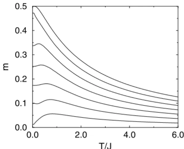
As a last example we show in Fig. 4 magnetization curves as a function of temperature for a spin ladder model.[18]
5
Coupling expansion
Histogram reweighting and Wang-Landau sampling can not only be applied to reweighting in the temperature but also to reweighting in the strength of a coupling constant. We will show as an example the SSE version.[9] Defining the Hamiltonian asH =H0+λV we can rewrite the partition function Eq. (29) as
Z=
∞
n=0
βn
n!Tr(−H0−λV)
n≡
∞
nλ=0
˜
0.0 2.0 4.0 6.0
T/J
0.0 0.1 0.2 0.3 0.4 0.5
m
Figure 4. Magnetization curve of an antiferromagnetic isotropic spin-1/2Heisenberg ladder as a function of temperature at varying magnetic fieldsh/J = 0,0.5,1,1.5,2,2.5,3.
0.00 0.20 0.40 0.60 0.80 1.00
J / J’
0.00 0.50 1.00 1.50 2.00
S
(
π,π
) /
L
2−
z
−
η
L=6
L=8
L=12
L=16
L=4
Figure 5. Scaling plot of the staggered structure factor of a Heisen-berg bilayer as a function of the coupling ratioλ=J/J′. Results
are shown for various linear system sizesL. The temperature was chosenβJ′ = 2L, low enough to be in the scaling regime. The
cutoffΛ = 8L3
was chosen large enough to cover the coupling rangeJ/J′ 1. The dynamical critical exponent of this model is
z= 1andη= 0.034.
where on the right hand side we have collected all terms as-sociated withλnλ
into˜g(nλ).
We consider as a first example thequantum phase transi-tionin a bilayer Heisenberg antiferromagnet whose ground state changes from quantum disordered to N´eel ordered as the ratio λ = J/J′ of intra-plane (J) to inter-plane (J′) coupling is increased [19]. From the histograms generated withinonesimulation we can calculate the staggered struc-ture factorS(π, π)of the system atany valueofλ. In Fig. 5 we show a scaling plot ofS(π, π)/L2−z−η as a function of
λ. In short simulations, taking only a few days on an 800 MHz Pentium-III CPU, we find the quantum critical point at
λ= 0.396, which again compares well with earlier results [19]. Statistical error bars are obtained from ten independent runs, and shown in Fig. 5 at selected values ofJ′/J.
As a final example we show magnetization curves for a spin flop transition in a two-dimensional quantum Heisen-berg antiferromagnet in Fig. 6.
1.7 1.8 1.9
h/J
0.000.05 0.10 0.15
m
Figure 6. Magnetization curve at the spin flop transition in a two-dimensional quantum spin-1/2 easy-axis antiferromagnet withJz/Jxy = 1.5at an inverse temperatureβJxy = 24
cal-culated by the quantum version of Wang-Landau sampling.
6
Conclusions
To summarize, we have shown how classical histogram reweighting and Wang-Landau sampling can be applied to quantum systems, allowing us to simulate quantum systems with similar accuracy as is possible for classical ones. This is possible in any representation, such as discrete or contin-uous time path integrals or in a stochastic series expansion (SSE) representation. At first order phase transitions we see, like in the classical case, a speedup of simulations by many orders of magnitude. These algorithms open up new possi-bilities for quantum Monte Carlo simulations.
We thank D.P. Landau for discussions and acknowledge support of the Swiss National Science Foundation. MT is grateful to the organizers of the third Brazilian Meeting on Simulational Physics for the invitation to visit their country.
References
[1] M. Suzukiet al., Prog. Theor. Phys.58, 1377 (1977); J.E. Hirschet al., Phys. Rev. Lett.47, 1628 (1981).
[2] R.H. Swendsen and J.-S. Wang, Phys. Rev. Lett. 58, 86 (1987); U. Wolff, Phys. Rev. Lett.62, 361 (1989).
[3] H.G. Evertzet al., Phys. Rev. Lett.70, 875 (1993).
[4] B. B. Beard and U. J. Wiese, Phys. Rev. Lett.77, 5130 (1996).
[5] A.W. Sandvik, Phys. Rev. B 59, R14157 (1999); O. F. Sylju˚asen and A. W. Sandvik, Phys. Rev. E 66, 046701 (2002).
[6] N. V. Prokof’evet al., Sov. Phys. - JETP87, 310 (1998).
[7] N. Prokof’ev and B. Svistunov, Phys. Rev. Lett.87, 160601 (2001).
[8] F. Wang and D.P. Landau, Phys. Rev. Lett.86, 2050 (2001); Phys. Rev. E64, 056101 (2001).
[9] M. Troyer, S. Wessel and F. Alet, Phys. Rev. Lett.90, 120201 (2003).
[11] B.A. Berg and T. Neuhaus, Phys. Rev. Lett.68, 9 (1992).
[12] P. Dayalet al., Preprint cond-mat/0306108.
[13] M. Suzuki, Prog. Theor. Phys.65, 1454 (1976).
[14] N.V. Prokof’evet al., Pis’ma v Zh.Eks. Teor. Fiz., 64, 853 (1996) [English translation is Report cond-mat/9612091].
[15] A.W. Sandvik and J. Kurkij¨arvi, Phys. Rev. B 43, 5950 (1991); A. W. Sandvik, J. Phys. A25, 3667 (1992).
[16] A.W. Sandvik, Phys. Rev. Lett.80, 5196 (1998).
[17] F. Hebertet al., Phys. Rev. B65, 014513 (2002).
[18] T. Barneset al., Phys. Rev. B47, 3196 (1993); M. Troyeret al., Phys. Rev. B50, 13515 (1994).