UNIVERSIDADE T´
ECNICA DE LISBOA
INSTITUTO SUPERIOR DE ECONOMIA E GEST ˜
AO
Mestrado em: Matem´
atica Financeira
COPULAS AND DEFAULTS WITHIN A CRISIS
CL ´
AUDIA CATARINA AC ´
URCIO DUARTE
Orienta¸c˜ao: Doutora Ana Isabel Pires Sarmento Lacerda
J´
uri:
Presidente: Doutor Onofre Alves Sim˜oes
Vogais: Doutor Jo˜ao Carlos Henrique da Costa Nicolau
Doutora Ana Isabel Pires Sarmento Lacerda
Abstract
In the aftermath of the subprime crisis, the main purpose of this thesis is to
as-sess the default dependency among firms, studying the case of four US financial
institutions in two periods of time: before and during the crisis. The methodology
followed is based on conditional copula models, which provides a set of global and
tail dependency measures, beyond the linear correlation widely misused in financial
problems. For this purpose, we use CDS (credit default swap) data to estimate the
copulas, that are assumed to be a proxy for default closeness, as they reflect the
credit risk of the institutions. As far as we know, this is a novelty of the present
analysis. The usual practice is to use equity returns, which are incomplete and more
indirect indicators of defaults. The procedures are carried out in two steps. First,
we model the individual dynamics for defaults closeness, by using ARMA-GARCH
specifications applied to CDS spreads variations and assuming t-distributed
innova-tions (to capture the extreme observainnova-tions). Then, we fit a set of copula funcinnova-tions
to the standardised residuals of the marginal distributions. The best specifications
for the characterisation of the dependency structure are different for the two
sub-periods analysed, confirming a structural break in the default dependency pattern,
occurred in the summer of 2007. The results also confirm our expectations regarding
the global dependency under stressful scenarios. For the four considered financial
institutions, all the dependency measures rose substantially in the crisis period.
Furthermore, we observe a significant increase in the upper tail dependency,
corre-sponding to high probabilities of simultaneous defaults. These outcomes point out
to the increase of the systemic and contagion risks in the US financial markets.
Keywords: Crisis, Copula, Default, Dependency, CDS spreads, ARMA-GARCH.
Resumo
No rescaldo da crise do subprime, o principal objectivo desta tese ´e avaliar a
de-pendˆencia entre os defaults de empresas, estudando o caso de quatro institui¸c˜oes
financeiras americanas em dois per´ıodos: antes e durante a crise. A metodologia
utilizada baseia-se em modelos de c´opulas condicionadas, que fornecem um conjunto
de medidas de dependˆencia global e de cauda, complementando a correla¸c˜ao linear
indevidamente utilizada nos problemas financeiros. Para esse efeito, usamos os CDS
para estimar c´opulas, que s˜ao assumidos comoproxy para a proximidade aodefault,
dado que reflectem o risco de cr´edito das institui¸c˜oes. Tanto quanto sabemos, esta
´e uma novidade da presente an´alise. A pr´atica usual ´e utilizar rendibilidades das
ac¸c˜oes, que s˜ao um indicador incompleto e mais indirecto dos defaults. Os
procedi-mentos s˜ao realizados em duas etapas. Primeiro, s˜ao modelizadas as dinˆamicas
indi-viduais para a proximidade aosdefaults, usando especifica¸c˜oes ARMA-GARCH para
as varia¸c˜oes dos CDS spreads e assumindo que as inova¸c˜oes seguem a distribui¸c˜ao
t-student (para captar as observa¸c˜oes extremas). De seguida, ajustamos um
con-junto de fun¸c˜oes c´opula para os res´ıduos standardizados das distribui¸c˜oes marginais.
As melhores especifica¸c˜oes para a caracteriza¸c˜ao da estrutura de dependˆencia s˜ao
diferentes para os dois sub-per´ıodos analisados, confirmando uma quebra estrutural
no padr˜ao de dependˆencia dos defaults, ocorrida no Ver˜ao de 2007. Os
resulta-dos tamb´em confirmam as nossas expectativas relativamente `a dependˆencia global
em cen´arios de stress. Para os quatro bancos considerados, todas as medidas de
dependˆencia aumentaram substancialmente no per´ıodo de crise. Al´em disso,
obser-vamos um aumento significativo da dependˆencia na cauda direita, o que corresponde
a uma elevada probabilidade dedefaults simultˆaneos. Estes resultados apontam para
o aumento do risco sist´emico e de cont´agio nos mercados financeiros dos EUA.
Palavras-Chave: Crise, Copula, Default, Dependˆencia, CDS spreads, ARMA-GARCH.
Contents
1 Introduction 8
2 Theoretical framework 14
2.1 Copulas . . . 14
2.1.1 Definition . . . 16
2.1.2 Measures of dependency . . . 18
2.1.3 Copula Families . . . 21
2.1.4 Calibration . . . 25
2.1.5 The conditional copula . . . 27
2.2 Applications to finance . . . 28
3 Empirical analysis 31 3.1 Data and Descriptive Statistics . . . 32
3.1.1 CDS spreads . . . 34
3.1.2 CDS spreads variation . . . 37
3.2 Empirical results . . . 39
3.2.1 Marginal densities . . . 42
3.2.2 Joint distributions using conditional copulas . . . 50
4 Summary and conclusions 59
Bibliography 64
List of Tables
3.1 Summary statistics of CDS spreads before the crisis (bp). . . 34
3.2 Summary statistics of CDS spreads during the crisis (bp). . . 35
3.3 Correlation matrix of CDS spreads before the crisis (bp). . . 35
3.4 Correlation matrix of CDS spreads during the crisis (bp). . . 35
3.5 ADF test for CDS spreads before the crisis. . . 36
3.6 ADF test for CDS spreads during the crisis. . . 36
3.7 Summary statistics of CDS spreads variation before the crisis (bp). . 37
3.8 Summary statistics of CDS spreads variation during the crisis (bp). . 37
3.9 Correlation matrix of CDS spreads variation before the crisis (bp). . . 38
3.10 Correlation matrix of CDS spreads variation during the crisis (bp). . 38
3.11 DF test for CDS spreads variation before the crisis. . . 40
3.12 DF test for CDS spreads variation during the crisis. . . 40
3.13 Jarque-Bera test for CDS spreads variation before the crisis. . . 40
3.14 Jarque-Bera test for CDS spreads variation during the crisis. . . 40
3.15 ARCH test for CDS spreads variation before the crisis. . . 41
3.16 ARCH test for CDS spreads variation during the crisis. . . 41
3.17 ARMA-GARCH models results, estimates (standard errors) for CDS spreads variation before the crisis. . . 44
3.18 ARMA-GARCH models results, estimates (standard errors) for CDS spreads variation during the crisis. . . 44
3.19 Ljung-Box test applied to the standardised residuals before the crisis. 45 3.20 Ljung-Box test applied to the standardised residuals during the crisis. 45 3.21 ARCH test for standardised residuals before the crisis. . . 45
3.22 ARCH test for standardised residuals during the crisis. . . 45
3.23 Linear correlation of the standardised residuals before the crisis . . . 47
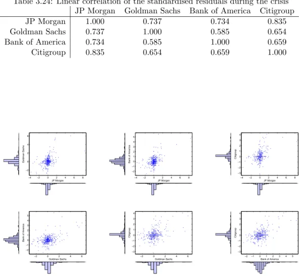
3.24 Linear correlation of the standardised residuals during the crisis . . . 47
3.25 Gaussian and T parameters for each pair of banks, before the crisis. . 51
3.26 Gaussian and T parameters for each pair of banks, during the crisis. . 51
3.28 Archimedean copula parameters (standard errors) for each pair of banks, during the crisis. . . 51 3.29 AIC criterion for each pair of banks, before the crisis. . . 52 3.30 AIC criterion for each pair of banks, during the crisis. . . 52 3.31 Rank correlation measures for T, Frank and Gumbel copulas, before
the crisis. . . 53 3.32 Rank correlation measures for T, Frank and Gumbel copulas, during
the crisis. . . 53
3.33 Confidence intervals for the estimates of the degrees of freedom (ν) of
the T-copula and for the parameters of Gumbel and Frank copulas, before and during the crisis. . . 54 3.34 Dependency measures according to the T copula, before the crisis. . . 57 3.35 Dependency measures according to the Frank copula, during the crisis. 57 3.36 Upper tail dependency coefficients according to the estimated Gumbel
List of Figures
1.1 Five stages of the crisis, BIS (2009) page 16. . . 10
3.1 CDS spreads before (left-hand side) and during the crisis (right-hand side). . . 34 3.2 ACF of CDS spreads before the crisis (bp), for JPMorgan, Goldman
Sachs, Bank of America and Citigroup, respectively. . . 36 3.3 ACF of CDS spreads during the crisis (bp), for JPMorgan, Goldman
Sachs, Bank of America and Citigroup, respectively. . . 36 3.4 CDS spreads variation before (left-hand side) and during the crisis
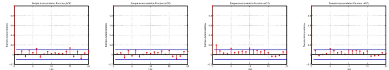
(right-hand side). . . 37 3.5 QQ-plots of the normal versus the empirical quantiles of CDS spreads
variation before the crisis (bp), for JPMorgan, Goldman Sachs, Bank of America and Citigroup, respectively. . . 40 3.6 QQ-plots of the normal versus the empirical quantiles of CDS spreads
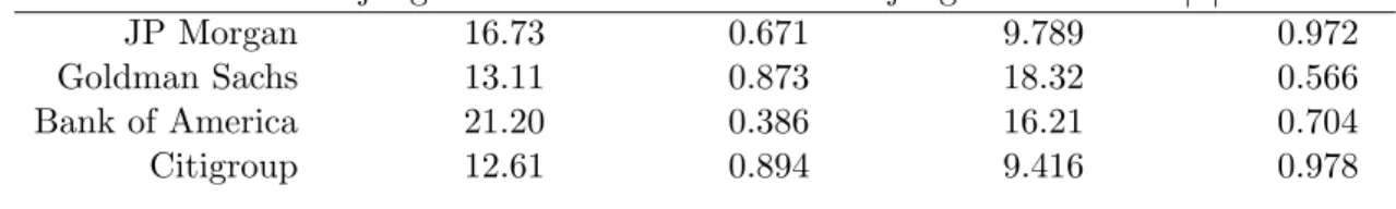
variation during the crisis (bp), for JPMorgan, Goldman Sachs, Bank of America and Citigroup, respectively. . . 40 3.7 ACF of CDS spreads variation before the crisis (bp), for JPMorgan,
Goldman Sachs, Bank of America and Citigroup, respectively. . . 41 3.8 PACF of CDS spreads variation before the crisis (bp), for JPMorgan,
Goldman Sachs, Bank of America and Citigroup, respectively. . . 41 3.9 ACF of CDS spreads variation during the crisis (bp), for JPMorgan,
Goldman Sachs, Bank of America and Citigroup, respectively. . . 41 3.10 PACF of CDS spreads variation during the crisis (bp), for JPMorgan,
Goldman Sachs, Bank of America and Citigroup, respectively. . . 41 3.11 Empirical distributions of standardised residuals, during the crisis.
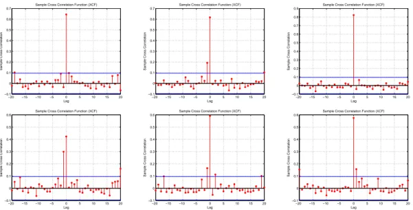
From the left-hand side to the right-hand side, JP Morgan, Goldman Sachs, Bank of America and Citigroup. . . 44 3.12 Cross-Correlograms of standardised residuals, during the crisis. Above,
3.13 Scatter plot of standardised residuals and the individual histograms, before the crisis, for each pair of institutions. . . 47 3.14 Scatter plot of standardised residuals and the individual histograms,
during the crisis, for each pair of institutions. . . 48 3.15 3-D Histograms for the standardised residuals and for the
correspond-ing uniform variables, for JPMorgan vs Citigroup, before the crisis. . 48 3.16 3-D Histograms for the standardised residuals and for the
correspond-ing uniform variables, for Goldman Sachs vs Bank of America, before the crisis. . . 48 3.17 3-D Histograms for the standardised residuals and for the
correspond-ing uniform variables, for JPMorgan vs Citigroup, durcorrespond-ing the crisis. . 49 3.18 3-D Histograms for the standardised residuals and for the
correspond-ing uniform variables, for Goldman Sachs vs Bank of America, durcorrespond-ing the crisis. . . 49 3.19 Probability and cumulative distribution functions, for JP Morgan vs
Citigroup, before the crisis, T copula. . . 55 3.20 Probability and cumulative distribution functions, for Goldman Sachs
vs Bank of America, before the crisis, T copula. . . 55 3.21 Probability and cumulative distribution functions, for JPMorgan vs
Citigroup, during the crisis, Frank copula. . . 55 3.22 Probability and cumulative distribution functions, for Goldman Sachs
vs Bank of America, during the crisis, Frank copula. . . 56
A.1 Time-varying parameter and Kendall’s tau, for JP Morgan vs Gold-man Sachs, during the crisis, Gumbel copula. . . 67 A.2 Time-varying parameter and Kendall’s tau, for JP Morgan vs Bank
of America, during the crisis, Gumbel copula. . . 67 A.3 Time-varying parameter and Kendall’s tau, for JP Morgan vs
Citi-group, during the crisis, Gumbel copula. . . 67 A.4 Time-varying parameter and Kendall’s tau, for Goldman Sachs vs
Bank of America, during the crisis, Gumbel copula. . . 68 A.5 Time-varying parameter and Kendall’s tau, for Goldman Sachs vs
Citigroup, during the crisis, Gumbel copula. . . 68 A.6 Time-varying parameter and Kendall’s tau, for Bank of America vs
Nomenclature
ACF Autocorrelation function
ADF Augmented Dickey-Fuller
AIC Akaike’s information criteria
ARCH Autoregressive conditional heteroscedasticity
ARMA Autoregressive moving average
BIS Bank for International Settlements
bp basis points
CDS Credit default swap
CML Canonical maximum likelihood
DF Dickey-Fuller
GARCH Generalised autoregressive conditional heteroscedasticity
IFM Inference functions for margins
IGARCH Integrated generalised autoregressive conditional heteroscedasticity
iid Independent and identically distributed
LB Ljung-Box
ML Maximum likelihood
Acknowledgments
Agradecimentos
⋆ A minha orientadora, Ana Lacerda, pela dedica¸c˜ao pessoal, disponibilidade e`
empenho na supervis˜ao da tese.
⋆ Aos colegas da Area de An´alise e Controlo Financeiro da Gest˜ao de Activas e´
Reservas do Banco de Portugal, pelo apoio incondicional, compreens˜ao e tempo disponibilizado. Em particular, ao colega Jo˜ao Pedro Brito, pela revis˜ao da tese e sugest˜oes pertinentes.
⋆ Ao Bruno Albuquerque, quer pela amizade demonstrada, quer pela leitura do
texto e respectivos coment´arios, sem esquecer os bons momentos proporciona-dos pelas discuss˜oes :-)
⋆ Ao Ant´onio Antunes, sempre prest´avel e ajuda imprescind´ıvel em tantas d´uvidas
que surgiram.
⋆ A Dora Leal, pelas trocas de impress˜oes muito ´` uteis sobre a metodologia.
⋆ To Rafael Guitart, by his support and useful comments regarding the writing
procedures.
⋆ Ao colega de mestrado Andr´e Ribeiro, por ouvir os desabafos em tantos
mo-mentos de desˆanimo.
⋆ Aos amigos em geral, pela aten¸c˜ao e paciˆencia nesta fase, especialmente `a
ˆ
Angela Salvador, que lidou diariamente com o problema :-)
⋆ Aos meus pais, que me apoiaram em todas as dificuldades e foram os grandes
respons´aveis pela manuten¸c˜ao da minha sanidade mental, ao longo do percurso efectuado!
⋆ A Funda¸c˜ao Econ´omicas, pela comparticipa¸c˜ao financeira do mestrado.`
⋆ A todos os que contribuiram directa ou indirectamente para o trabalho, que n˜ao
Chapter 1
Introduction
How could this happen? No one thought that the financial system could collapse...
The modern financial system is immensely complex - possible too complex for any
person to really understand it. Interconnections create systemic risks that are
ex-traordinary difficult to figure out. The fact that things apparently worked so well ...
gave everyone a false sense of comfort.1
Economic crises are the result of years, even decades, of global economic change,
imbalances accumulation, policy errors and investor misjudgement. Although these
crisis never happen overnight, there is always a moment when the world seems to
be upside down, faced with a dramatic loss of confidence. The bankruptcy of the
158-years-old firm Lehman Brothers, on 15 September 2008, was indeed one of those
such moments, corresponding to the worst point of the financial crisis and plunging
the world economy in to what seems to be the most dangerous recession, since the
Great Depression of the late 1920s.
Modern life style requires an appropriate and reliable functioning of the financial
system, composed of banks, insurance companies, governments, pension funds and
securities firms. Around the middle of the current decade, the financial world system
seemed to be working perfectly. Prosperity and stabilisation were evidenced in the
main economic indicators, with inflation kept at low levels and economic growth
ex-1
hibiting a sustainable rate. In addition, central banks were providing liquidity to the
market, lending to banks when needed, deposit insurance and investors protections
schemes were in place and regulators and supervisors were, apparently, comfortable
with the risk taken by financial institutions.
However, when the house prices began their steep decline, after their peak in
mid-2006, refinancing became more difficult. Securities backed with subprime
mort-gages,2 widely held by financial institutions, lost most of their value resulting in a
large decline in the capital of many banks and U.S. government sponsored agencies,
in particular, Freddie Mac and Fannie Mae. The subprime crisis had begun. The
losses were even higher than expected, as many banks have hidden their holdings
of sub-prime mortgages in exotic, off-balance sheet instruments such as structured
investment vehicles. The lack of confidence between banks, evidenced by the
un-willingness to lend to each other, was a clear sign of the collapse, prevailing a huge
panic in financial markets and in economies in general. Bear Stearns was rescued in
March 20083 and, six months later, it was the Lehman Brothers bankruptcy. In fact,
since then, the complex financial system has been critically hampered to its core.
Public bailouts of financial institutions and massive economic support packages as
well as unconventional liquidity support measures by central banks, to restore the
global financial markets, remind the vulnerability of the system and the importance
of keeping it healthy. This unprecedent intervention of central banks and
govern-ments was fundamental to avoid a more severe and lasting recession. However, such
monetary policies and government actions, for instance, the very low level of interest
rates, bank rescues, fiscal stimulus programs and bailouts, cannot be maintained for
too long, to avoid future asset-price bubbles and other destabilising phenomena.
Media, literature, investigators often inquire on the causes of the current crisis.
The increased risk-taking and leverage, due to the long period of low real interest
rates are commonly presented as reasons. The global imbalances and the dependency
2
The subprime home loans are provided to borrowers with poor credit histories and weak documentation of income.
3
between the export emerging countries and industrial economies that, at least,
wors-ened and extended the crisis reach and duration. From a microeconomic point of
view, several factors were also pointed out. Among them, it should be stressed, on
the one hand, the dangerous incentives for investors and for financial sector
employ-ees and, on the other hand, the lack of impartiality in ratings assignment, depending
on who pays and needs them the most; the flaws in techniques4 used to measure,
price and manage risk and in corporate governance structures used to monitor it;
and the shortfalls of the regulatory systems.
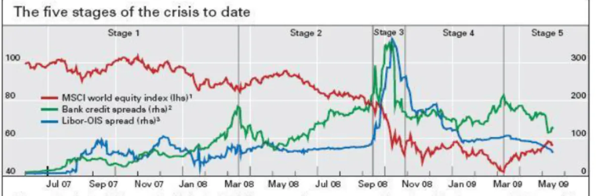
Figure 1.1: Five stages of the crisis, BIS (2009) page 16.
The aforementioned reasons were the ground for a severe financial crisis, with
deep implications on the economic activity. Figure 1 presents an indicative
section-ing of the crisis period:
1. Pre-March 2008: prelude of the crisis, leading up to the takeover of Bear Sterns;
2. Mid-March to mid-September 2008: towards the Lehman bankruptcy, credit
default swaps (CDS) spreads increased substantially;
3. 15 September to late October 2008: global loss of confidence, a growing number
of financial institutions were facing risk of default, large scale bank rescues,
deposit and debt guarantees;
4
4. Late October 2008 to mid-March 2009: global downturn - declines in GDP,
inflation falls, huge fiscal stimulus packages were announced by governments,
rates cut to near zero levels, outright purchases of public and corporate debt;
5. Since mid-March 2009: downturn deepens but loses speed, first signs of
stabil-isation, volatilities have declined but persistent signs of dysfunction in markets
remain.
In this context, for the years 2007-2008, the following key events should be
high-lighted:
⋆ July/August 2007 - Liquidity crisis
⋆ November 2007 - Northern Rock collapse
⋆ March 2008 - Bear Sterns takeover
⋆ September/October 2008 - Lehman bankruptcy
The behaviour of the average CDS spreads for 18 major international banks
(see figure 1) reflect these key events, seeming to provide a reliable indicator of the
magnitude of the crisis.
Under this scenario, an accurate measure of credit risk and default dependency
between institutions became an absolute need. Lehman Brothers filled the largest
bankruptcy in history and it was followed by a large number of institutions. This
phenomenon was not predicted in credit risk products whose pool of collateral
even-tually did not include Lehman, but included some of related institutions’ debt that
certainly were affected by the Lehman fall-out. Hence, estimating dependencies is
really important, because under stressful conditions the mispecification of
diversi-fication can be crucially dangerous to portfolio returns. Throughout the crisis, the
early warning signals of deteriorating credit quality, materialised in CDS spreads,
as well as the evidence of bankruptcies are obvious issues to study.
In this context, the main goal of the thesis is to understand the association and
default dependencies among financial institutions, before and during the crisis,
modelling, which is a novelty of the present work, as far as we know. An usual
prac-tice is to assume that default probabilities share the same dependency structure
than equity returns and use them to fit the copula.5 However, in this thesis, CDS
spreads are used because they are a more direct and complete indicator of defaults
than equity data, confirmed by their increasing liquidity of the last years. In fact,
when the price of a CDS goes up, it indicates that default risk has risen. Our
analy-sis is carried out using the CDS spreads of four US institutions, namely, JP Morgan
Chase & Co., Goldman Sachs Inc, Bank of America Corp and Citigroup Inc. The
relationship between these institutions is studied for two periods: before the crisis,
since January 2006 until July 2007, and during the crisis, since August 2007 until
March 2009. The work follows Dias and Embrechts (2003) and Palaro and Hotta
(2006) to explore dependency concepts through conditional copula models. Firstly,
the individuals default behaviour is specified using the CDS spreads variations of
the corresponding institutions to fit ARMA-GARCH models. Then, based on
con-ditional copula-approach, the residuals of default dynamics are the inputs used to
evaluate the default dependency between the considered institutions. The measures
of dependency based on rank correlation and tail dependency are taken into account
beyond the correlation estimates commonly used.
The remainder of the text is organised as follows. Chapter 2 describes the
the-oretical framework needed to understand copulas as a tool to capture dependencies
between random variables. In particular, in section 2.1 is presented a survey on
copula related definitions, properties and dependency measures, such as global and
tail dependency, and their suitability compared to linear correlation. In addition,
we review a set of elliptical and Archimedean copula specifications, as well as the
estimation procedures based on maximum likelihood. At the end of the section,
the conditional copula framework is introduced. In section 2.2, the application of
copulas to finance and some references are pointed out. Chapter 3 presents all the
empirical study, repeating the procedures for the two periods considered, before and
during the crisis, for each of the six pairs composed by four US financial institutions:
5
JP Morgan Chase, Goldman Sachs, Bank of America and Citigroup. In section 3.1,
the CDS data is analysed and all the pre-model work is explained, including the
differentiation of CDS spreads to obtain stationary series. Section 3.2 implements
the individual dynamics for CDS spreads variations, through ARMA-GARCH
mod-els, assuming t-distribution for innovations, and tests their adequacy. In addition, a
set of copula models are fitted evaluating the t-cumulative distribution function at
the standardised residuals from the ARMA-GARCH modelling. The AIC criterion
ranks the estimated copulas and the confidence intervals are calculated to ensure
robustness of copula parameters estimates. Given the selected copulas, we interpret
the global and tail dependency measures before and during the crisis, for the pairs
of institutions considered. Finally, section 4 presents a summary of the results and
suggestions of future investigation. In appendix A we illustrate a particular dynamic
copula which is compared with the corresponding static one, to motivate the study
Chapter 2
Theoretical framework
This chapter provides an introduction to the copula theory. In section 2.1 we review
the theoretical background on copula function, while in section 2.2 some references
of empirical applications to finance are presented.
2.1
Copulas
The term copula comes from the Latin noun which means “link, tie, bond”,i.e.,
join-ing together. A copula is a function which marries a group of univariate marginal
distribution functions into a multivariate distribution function, capturing the
rela-tionship between random variables. Every joint distribution function of a set of risk
factors implicitly contains a description of the marginal behaviour of individual risk
factors and a description of their dependency structure. Copula functions provide
a way of isolating the dependency structure and to express it on a quantile scale,
which is useful for describing the dependency of extreme outcomes and, naturally,
to use in a risk-management context.
Copula functions, introduced in 1959, are the most general way to view
depen-dency of random variables. They provide a number of useful alternative measures of
dependency to the linear correlation coefficient, which often fail to capture important
risks. In fact, correlation is widely misused in finance, being applied to problems for
the interval [−1,1], is defined as
ρ(Y1, Y2) =
Cov(Y1, Y2)
p
V ar(Y1)
p
V ar(Y2)
,
whereY1 and Y2 are random variables.
The linear correlation coefficient merely captures the linear dependency. Two
perfectly dependent variables exhibit a correlation coefficient of +1 or−1,
depend-ing on the variables bedepend-ing positively (i.e., rise or fall together) or negatively
de-pendent, respectively. The closer the coefficient is to either −1 or 1, the stronger
the correlation. If the variables are independent, the linear correlation coefficient is
zero, but the converse is not true, with the exception being the variables whose joint
distribution is normal. For other cases the linear correlation can be an imperfect
measure of dependency. This measure presents several limitations, as it is not
invari-ant under non-linear transformations of the random variables and it is not defined
when variances approach to infinite, which is the case of heavy-tailed distributions.
As in financial series there is strong dependency among big losses (gains), this is an
important drawback of correlation.
Furthermore, according to Elizalde (2005), the conclusions extracted from the
comparison of linear default correlations should be read carefully. In fact, these
measures are covariance-based and do not make sense for joint non-elliptical random
variables1 such as default events. The use of copula based measures of dependency
can overcome this limitation. Unlike correlation, copulas are invariant under strictly
increasing transformations of risks and allows us to model asymmetries, as we will
see below. For a more detailed description of copula theory see McNeil et al. (2005),
Nelsen (1999) and Embrechts et al. (2001).
1
IfY is a n-dimensional random vector, for someµ∈Rnand somen×nnonnegative definite, symmetric
matrix Σ, the characteristic functionψY−µ(t) of (Y−µ) is a function of the quadratic formtTΣt. SoY has
an elliptical distribution with parametersµ, Σ andψ. t-student and normal distributions are examples of
elliptical distributions. Even for jointly elliptically distributed random variables there are situations where using linear correlation does not make sense, for example, when there is infinite second moments such as
2.1.1 Definition
A copula functionCis the joint distribution of a set of N uniform random variables
U1, . . . , UN, allowing to separate the modelling of the marginal distribution functions
from the modelling of the dependency structure. The choice of the copula does not
constrain the choice of the marginal densities and vice-versa. Moreover, copulas
differ not so much in the degree of association they provide, but rather in which
part of the distributions the association is strongest.
A formal definition of a copula function is as follows:
Definition 1. A N-dimensional copula is a function C : [0,1]N → [0,1] satisfying
the conditions:
• For all (u1, . . . , uN) in [0,1]N, if at least one component ui is zero, then
C(u1, u2, . . . , uN) = 0.
• For ui ∈[0,1], C(1, . . . ,1, ui,1. . . ,1) =ui for all i∈ {1,2, . . . , N}.
• For all[u11, u12]×[u21, u22]×. . .×[uN1, uN2]N-dimensional rectangles in[0,1]N,
2
X
i1=1
2
X
i2=1
· · ·
2
X
iN=1
(−1)i1+i2+...+iNC(u
1i1, u2i2. . . , uN iN)≥0.
An alternative and more intuitive definition of a copula function is presented in
Sch¨onbucher (2003):
Definition 2. A functionC: [0,1]N →[0,1]is a copula if there are uniform random
variables U1, . . . , UN taking values in [0,1] such that C is their joint distribution
function.
The Sklar’s Theorem(1959) shows that any multivariate distribution function F
can be written as a copula function. Formally,
Theorem 3. (Sklar) Let Y1, Y2, . . . , YN be random variables with marginal
N-dimensional copula C such that for(y1, y2, . . . , yN)∈RN we have
F(y1, y2, . . . , yN) = P[Y1 ≤y1, Y2 ≤y2, . . . , YN ≤yN] =C(F1(y1), F2(y2), . . . , FN(yN)).
(2.1)
Additionally, if each Fi is continuous, the copula C is unique.
Sklar’s theorem expresses the basic idea of dependency modelling via copula
functions by stating that, for any multivariate distribution function, the
univari-ate margins (the distribution functions of random variables) and the dependency
structure can be separated, with the latter being completely described by a
cop-ula function. This theorem has the following important corollary for simcop-ulation
purposes:
Corollary 4. Let F and C be, respectively, a N-dimensional distribution function
(with continuous univariate margins F1, F2, . . . , FN) and a N-dimensional copula
function. Then, for any u∈[0,1]N, we have
C(u1, u2, . . . , uN) =F(F1−1(u1), F2−1(u2), . . . , FN−1(uN)), (2.2)
where Fi−1(ui) denotes the inverse of the cumulative distribution function, namely,
for ui ∈[0,1], Fi−1(ui) = inf{y:Fi(y)≥ui}.
Corollary 5. Applying Sklar’s theorem and using the relation between the
dis-tribution and the density function, we can derive the multivariate copula density
c(F1(y1), . . . , FN(yN)) associated with a copula function C(F1(y1), . . . , FN(yN)):
f(y1, . . . , yN) =
∂N[C(F
1(y1), . . . , FN(yN))]
∂F1(y1). . . ∂FN(yN) ·
f1(y1). . . fN(yN)
= c(F1(y1), . . . , FN(yN))·f1(y1). . . fN(yN), (2.3)
where we define
c(F1(y1), . . . , FN(yN)) =
∂N[C(u
1, . . . , uN)]
∂u1. . . ∂uN
= f(y1, . . . , yN)
f1(y1). . . fN(yN)
The associated copula density is particulary useful to calibrate its parameters to
real market data.
Remark 6. Consider a pair of uniform (0,1) random variables (U, V) with copula
C. We have
P(V ≤v|U =u) = ∂
∂uC(u, v); (2.4)
C(u,1) =P(U ≤u, V ≤1) = P(U ≤u) =u; (2.5)
and
C(u,0) =P(U ≤u, V ≤0) = 0. (2.6)
2.1.2 Measures of dependency
Since each marginal distribution Fi contains all the univariate information on the
individual variableYi and the joint distribution functionF contains all the univariate
and multivariate information, the information contained on the copula C respects
the dependency between the marginal distributions (Yi variables).
The dependency between variables can be assessed with different measures. On
the one hand, we have the linear correlation and, on the other hand, we have copula
based dependency measures, such as rank correlation coefficients (Kendall’s tau and
Spearman’s rho) and coefficients of tail dependency. Some measures of association
are only dependent on the copula and not on the marginal distributions. As we
have already mentioned, the linear correlation coefficient, the most used measure of
dependency, measures the overall strength of the association but does not provide
information on the variation of this association across the distribution. Furthermore,
unlike linear correlation, rank correlation and tail dependency coefficients do not
depend on the marginal distributions.
The characteristics of the data and the respective dependency measures can
suggest the copula specification to choose. In particular, these measures indicate
the part of the distributions where variables are more associated, specially in the
tails, which represent, for example, correlation among large losses.
significant part of the theoretical framework, including the dependency measures, is
explained for the bivariate case.
Rank correlation
Rank correlations are simple scalar association measures that only depend on the
copula of a bivariate distribution. The standard empirical estimators of rank
corre-lation may be calculated only by analysing the ranks of the data, regardless of the
actual numerical values.
Definition 7. Concordance Let (y1, y2) and (y′
1, y′2) be two observations from a
vector (Y1, Y2) of continuous random variables. Then, (y1, y2) and (y1′, y′2) are said
to be concordant if (y1−y′1)(y2−y′2)>0 and discordant if (y1−y1′)(y2−y2′)<0.
Intuitively, if Y2 tends to increase with Y1, then we expect that the probability
of concordance to be high relative to the probability of discordance; ifY2 tends to
increase with the decreasing ofY1, then we expect the opposite.
Kendall’s tau and Spearman’s rho are two measures of dependency, based on the
concordance concept.
Definition 8. Let (Y1, Y2) and (Y1′, Y2′) be i.i.d. random vectors of continuous
ran-dom variables with the same joint distribution function given by the copula C (and
with marginals F1 and F2). Then, Kendall’s tau of the vector (Y1, Y2) (and of the
copula C) is defined as the probability of concordance minus the probability of
dis-cordance, i.e.
τ = P[(Y1−Y1′)(Y2−Y2′)>0]−P[(Y1−Y1′)(Y2−Y2′)<0] (2.7)
= 4
Z Z
[0,1]2
C(u, v)dC(u, v)−1
= 1−4
Z Z
[0,1]2
∂C(u, v)
∂u
∂C(u, v)
∂v dudv. (2.8)
Definition 9. Let (Y1, Y2), (Y1′, Y2′)and(Y1′′, Y2′′)be i.i.d. random vectors of
contin-uous random variables with the same joint distribution function given by the copula
of the copula C) is defined as
ρS = 3(P[(Y1−Y1′)(Y2−Y2′′)>0]−P[(Y1−Y1′)(Y2 −Y2′′)<0]) (2.9)
= 12
Z Z
[0,1]2
uvdC(u, v)−3
= 12
Z Z
[0,1]2
C(u, v)dudv−3. (2.10)
Spearman’s rho can be interpreted as the linear correlation between distribution
functions of random variables. Let (Y1, Y2) be a random vector of continuous random
variables with the same joint distribution function H (whose margins are F1 and
F2) and copula C, and consider the random variables U = F(Y1) and V = F(Y2).
Therefore, we can write the Spearman’s rho coefficient of (Y1, Y2) as
ρS(Y1, Y2) = 12
Z Z
[0,1]2
uvdC(u, v)−3 = 12E[U V]−3 = E[U V]−1/4
1/12
= p Cov(U, V)
V ar(U)V ar(V) =ρ(U, V) =ρ(F1(Y1), F2(Y2)),
where ρ denotes the linear correlation coefficient. So, the Spearman’s rho of the
vector (Y1, Y2) is the Pearson correlation of the random variablesF1(Y1) andF2(Y2).
These rank measures of dependency take values that belong to the interval [−1,1].
It equals−1 if the two random variables are countermonotonic; equals 1 if they are
comonotonic and, equals 0 if they are independent.
Tail dependency
Kendall’s tau and Spearman’s rho are measures of global dependency. In
con-trast, tail dependency coefficients between two random variables (Y1, Y2) are
lo-cal/extremal measures of dependency, as they refer to the level of dependency
be-tween extreme values,i.e., the tails of the distributionsF1(Y1) and F2(Y2).
Copulas have a flexible structure that allow for tail dependency, which is a very
important feature to study correlated defaults in crisis periods. The concept of tail
dependency is specified for each tail and it relates to the amount of dependency in the
addressing upper tail dependency, lower tail dependency or both.
The coefficients we describe are defined in terms of limiting conditional
proba-bilities ofquantile exceedances.
Definition 10. Let (Y1, Y2) be a random vector of continuous random variables
with copula C (and with marginals F1 and F2). Then, the coefficient of upper tail
dependency of the vector (Y1, Y2) (and of the copula C) is defined as
λU = lim
u→1P[Y1 > F
−1
1 (u)|Y2 > F2−1(u)] (2.11)
= lim
u→1
1−P[Y1 ≤F1−1(u)]−P[Y2 ≤F2−1(u)] +P[Y1 ≤F1−1(u), Y2 ≤F2−1(u)]
1−P[Y2 ≤F2−1(u)]
= lim
u→1
1−2u+C(u, u)
1−u (2.12)
whereFi−1 represents the inverse function ofFi, provided the limit exist. We say that
the random vector (and copula C) has upper tail dependency if λU > 0. Similarly,
the coefficient of lower tail dependency of the vector(Y1, Y2)(and copulaC) is defined
as
λL= lim
u→0P[Y1 < F
−1
1 (u)|Y2 < F2−1(u)] = lim
u→0
C(u, u)
u . (2.13)
We say that the random vector (and copulaC) has lower tail dependency if λL >0.
Upper (lower) tail dependency measures the probability of a component of the
vector (Y1, Y2) to be extremely large (small) given that the other is extremely large
(small). Intuitively, upper (lower) tail dependency exists when there is a positive
probability of positive (negative) outliers occurring jointly.
If λU = 0 (λL = 0), then the two random variables (Y1, Y2) are said to be
asymptotically independent in the upper (lower) tail.
2.1.3 Copula Families
This subsection surveys some of the copula functions most used in default risk
modelling. First, we present the Gaussian and T-copulas, which belong to the
Multivariate Gaussian Copula
The N-dimensional Gaussian copula with covariance matrix Σ is given by
C(u1, . . . , uN) = ΦNΣ(Φ−1(u1), . . . ,Φ−1(uN)), (2.14)
where ΦN
Σ represents a N-dimensional normal distribution function, with Σ and Φ−1
denoting the covariance matrix and the inverse of the univariate normal distribution
function, respectively.
Normal copulas are radially symmetric (λU =λL), tail independent (λU =λL =
0). Furthermore, the linear correlation coefficient ρ can be expressed in terms of
both Kendall’s tau (τ) and Spearman’s rho (ρS): ρ= 2 sin(π6ρS) = sin(π2τ).
As with any other copula, the normal copula enables the use of any marginal
distribution.
Multivariate Student’s T-Copula
Let X be a random vector distributed as a N-dimensional multivariate t-student
with ν degrees of freedom, mean vector µ (for ν > 1) and covariance matrix ν
ν−2Σ
(forν > 2). X can be expressed as
X =µ+
√
ν
√
SZ, (2.15)
where S is a random variable χ2-distributed with ν degrees of freedom and Z
is a N-dimensional normal random vector, independent of S, with zero mean and
covariance matrix Σ. The N-dimensional T-copula of X is given by
C(u1, . . . , uN) = tNν,R(tν−1(u1), . . . , t−ν1(uN)), (2.16)
where tN
ν,R is the distribution function of
√
ν
√
SZ, Z is a N-dimensional normal
random vector, independent of S, with zero mean and covariance matrix Σ. t−1
ν
denotes the inverse of the univariate t-student distribution function with ν degrees
of freedom and Rij = √ΣΣij
iiΣjj
The T-copula is radially symmetric and has tail dependency given by
λU =λL = 2−2tν+1
(ν+ 1)(1−ρ)
1 +ρ
1/2
, (2.17)
where ρ is the linear correlation of the bivariate t-distribution. The coefficient
of upper (lower) tail dependency is increasing in ρ and decreasing in ν. For ρ < 1,
it tends to zero as the number of degrees of freedom tends to infinity (Embrechts
et al. (2001)).
Archimedean copulas
Archimedean copulas constitute an important class of copula functions due to their
analytical tractability (many of them have closed form expression), parsimoniously
and variety of different dependency structures.
Let us consider a function ϕ : [0,1] → [0,∞], continuous, ϕ′(u) < 0 for all
u∈ [0,1] and ϕ(1) = 0. We then define pseudo-inverse of ϕ as the function ϕ[−1] :
[0,∞]→[0,1] such that:
ϕ[−1](t) =
ϕ[−1] for 0≤t≤ϕ(0)
0 for ϕ(0) ≤t≤ ∞
If ϕ is convex, then the function C: [0,1]2 →[0,1] defined as
C(u1, u2) = ϕ[−1][ϕ(u1) +ϕ(u2)] (2.18)
is an Archimedean copula andϕ is called the generator of the copula. Moreover,
if ϕ(0) = ∞, the pseudo-inverse describes an ordinary inverse function (that is
ϕ[−1] = ϕ−1) and we call ϕ and C, respectively, a strict generator and a strict
⋆ Gumbel Copula. Let ϕ(t) = (−lnt)θ with θ ≥ 1 and independency for
θ = 1. Then we have
CGumbelθ (u1, u2) = exp{−[(−lnu1)θ+ (−lnu2)θ]1/θ}.
⋆ Clayton Copula. Let ϕ(t) = (t−θ −1)/θ with θ ≥ −1, strict for θ ≥ 0 and
independency for θ= 0. Then,
CClaytonθ (u1, u2) = max[(u−1θ+u−2θ−1)−1/θ,0].
⋆ Frank Copula. Let ϕ(t) = −lne−θt
−1
e−θ−1 with θ ∈R\{0} and independency for
θ = 0. Then we obtain the following expression for copula
CF rankθ (u1, u2) =−
1
θln
1 + (e−
θu1
−1)(e−θu2
−1)
e−θ−1
.
For this family of copulas, tail dependency and Kendall’s tau coefficients can be
expressed in terms of the generator function,2
τ = 1 + 4
Z 1 0
φ(u)
φ′(u)du, (2.19)
λU = 2−2 lim
u→0
φ−1′ (2u)
φ−1′
(u) , (2.20)
λL = 2 lim
u→∞
φ−1′ (2u)
φ−1′
(u) . (2.21)
provided that the limits exist.
The Clayton copula has lower tail dependency (2−1/θ) but not upper tail
depen-dency andτ = θ+2θ . The Gumbel copula only has upper tail dependency (2−21/θ)
and τ = 1−1/θ. The Frank copula has neither upper nor lower tail dependency
and τ = 1 + 4D1(θ)−1
θ , where D1(θ) is the first order Debye function, defined as
D1(θ) = 1θ
Rθ
0
t
exp(t)−1dt. For these copulas, the larger the parameter θ (in absolute
value), the stronger the dependency structure.
2
In the Archimedean copulas framework, the dependency between any two random
variables does not depend on which variables we choose. Hence, the parameters do
not have a straightforward meaning in multivariate data. In terms of credit risk
analysis, this imposes an important restriction on the dependency structure since
the default dependency is the same between any set of firms. This is precisely the
reason for using pairs of variables in the empirical application.
2.1.4 Calibration
This subsection presents the main methods to calibrate copula parameters proposed
in statistical literature.3 In the following analysis consider a random sample
rep-resented by the time series Y = (Y1,t, Y2,t, . . . , YN,t)Tt=1, where N is the number
of underlying assets (firms) included and T represents the number of observations
available on a periodic (daily) basis.
The maximum likelihood (ML) method
Let Θ be the parameter space andθ be the k-dimensional vector of parameters to
be estimated. Let Lt(θ) and lt(θ) be, respectively, the likelihood and log-likelihood
for the observation at timet. The log-likelihood function l(θ) is defined as
l(θ) = ΣTt=1lt(θ). (2.22)
Expanding the previous expression using the copula function presented in
equa-tion (2.3), we obtain
l(θ) = ΣTt=1lnc(F1(y1t), . . . , FN(yNt )) + ΣTt=1ΣNi=1lnfi(yti). (2.23)
Then, the maximum likelihood estimator is defined as the vector ˆθ such that
ˆ
θ:= (ˆθ1, . . . ,θˆk)∈arg max{l(θ) :θ ∈Θ}.
3
As the ML estimates the dependency structure and the margins parameters
simultaneously, it is computationally very intensive. Therefore, two alternative
methodologies follow.
The inference functions for margins (IFM) method
According to this method,4 the parameters of marginal distributions are estimated
separately from the parameters of the dependency structure. The log-likelihood
functionl(θ) presented in equation (2.23) is expressed as follows
l(θ) = ΣTt=1lnc(F1(y1t;θ1), . . . , FN(yNt ;θN);α) + ΣTt=1ΣNi=1lnfi(yit;θi). (2.24)
In the above expression, the separation between the vector of the parameters for the
univariate marginals θ = (θ1, . . . , θN) and the vector of the copula parameters α is
clear. Summing up, the estimation process is dived into two steps:
1. Estimation of the vector of the parameters for univariate marginalsθ = (θ1, . . . , θN)
using ML method. For example, for the i− th underlying asset, we have
ˆ
θi = arg maxθi
PT
t=1lnfi(yit;θi).
2. Estimation of the vector of the copula parameters α using the previous
esti-mators ˆθ = (ˆθ1, . . . ,θˆN):
ˆ
αIF M = arg max
α Σ T
t=1lnc(F1(y1t; ˆθ1), . . . , FN(yNt ; ˆθN);α).
The IFM estimator5 is then defined as the vectorθIF M = (ˆθ,αˆ
IF M).
The canonical maximum likelihood (CML) method
Both ML and IFM methods are based on an exogenous imposition of a parametric
form of the univariate marginals. The CML differs from the IFM method because
4
Joe and Xu (1996).
5
no assumptions are needed about the parametric form of the marginal
distribu-tions. This method relies on the concept of empirical marginal transformation.
This transformation tends to approximate6 the marginals ˆF
i, fori= 1, . . . , N, with
the empirical distribution functions ˆFi(·) defined as
ˆ
Fi(·) =
1
TΣ
T
t=11{Yit≤·}, f or i= 1, . . . , N, (2.25)
where 1{·}represents the indicator function. The CML method is performed into
two steps:
1. Transformation of the initial data set Y = (Y1t, . . . , YN t)Tt=1 into uniform
variables, using the empirical marginal distribution described above, i.e., for
t = 1, . . . , T, let ˆut = (ˆut1, . . . ,uˆtN) = [ ˆF1(Y1t), . . . ,FˆN(YN t)].
2. Estimation of the vector of copula parameters α using the following relation:
ˆ
αCM L = arg max
α Σ T
t=1lnc(ˆut1, . . . ,uˆtN;α).
The CML estimator is then defined as the vectorθCM L = ˆα
CM L.
2.1.5 The conditional copula
This is an extension of some of the early applications of copulas in statistical
mod-elling where the random vector of interest could be assumed to be independent and
identically distributed (iid).
The conditional likelihood is given by the conditional version of the Sklar’s
The-orem 3. LetFi be the conditional distribution of Yi|W fori= 1, . . . , N,W be some
information set andF be the joint (absolutely continuous) conditional distribution
of Y|W, whereY = (Y1, . . . , YN) has conditional copula function C. Then,
F(y1, . . . , yN|w) = C(F1(y1|w), . . . , FN(yN|w)|w).
6
with the following adaptation of Corollary 5:
f(y1, . . . , yN|w) =c(F1(y1|w), . . . , FN(yI|w)|w) N
Y
i=1
fi(yi|w), (2.26)
where fi(yi|w) is the conditional density of Yi|W =w and
c(u1, . . . , uN|w) =
∂NC(u
1, . . . , uN|w)
∂u1. . . ∂uN
.
The log-likelihood expression that is equivalent to the one presented in equation
(2.23) is given by:
l(θ) = ΣTt=1lnc(F1(y1t|wt), . . . , FN(yNt |wt)|wt) + ΣTt=1ΣNi=1lnfi(yit|wt). (2.27)
and we can follow all the previous procedures in order to estimate the parameters.
An important restriction introduced of Sklar’s theorem applied to conditional
distributions is that the conditioning set, W, must be the same for all marginal
distributions and for the copula.
2.2
Applications to finance
Copulas are used in several scientific areas, for instance, mathematics, statistics,
biostatistics, operations research, natural sciences, engineering, actuarial science,
economics and finance. Nelsen (1999) is one of the standard books of copulas
com-bining the most important theorems and fundamental results about this subject.
Following this publication, the interest in applying copula methodology to finance
increased substantially. In fact, in June 2006, finance and actuarial science
to-gether contributed 47% of the literature7 about copulas. In the financial area, the
first research group in copulas, which was headed by Paul Embrechts and Mc Neill,
published several very cited papers about using copulas in risk management.8 At
the same time, Li (2000) developed a pioneer work about default correlation that
7
Genest et al. (2009).
8
models the random variable “time-until-default” and the survival functions, using
a Gaussian copula function. Other important references in the financial area, for
mathematical and intuitive framework, are Sch¨onbucher (2003), Duffie and
Single-ton (2003), Lando (2004) and, more recently, McNeil et al. (2005), which combines
copula theory and extreme value theory in the context of credit, market, operational
risks and insurance.
Nowadays, copulas are widely used in finance.9 Indeed, according to the database
presented in Genest et al. (2009), the major areas of application in finance are the
following, with some references:
⋆ Risk Management: Credit, market, operational risks and risk aggregation. See
Embrechts et al. (1999), Li (2000) and McNeil et al. (2005);
⋆ Portfolio Management: Dependency between financial markets, different assets
and currencies. See, for example, Patton (2004) and Dias and Embrechts
(2003);
⋆ Pricing of derivatives: CDS, CDO and other credit risk products. Some
refer-ences: Meneguzzo and Vecchiato (2002), Galiani (2003), Bluhm (2003),
Cheru-bini et al. (2004), Hull and White (2006), Hull and White (2007), Hull and
White (2008) and Hitier and Huber (2009);
⋆ Risk measurement: value-at-risk (VaR), expected shortfall (conditional VaR)
and financial contagion. See, for example, Embrechts et al. (2003) and Palaro
and Hotta (2006).
A topic that has captured the attention of finance researchers using copula
meth-ods is the study of financial contagion.10 As copulas contain all the information
about the dependency structure of a vector of random variables, they can capture
nonlinear dependency among variables and, in particular, in the tails of the
distri-bution. This is of extreme importance in periods of high levels of volatility in which
9
The websitewww.defaultrisk.com provides a substantial set of free downloadable papers on credit risk
and, in particular, contagion and dependency. Some of the references mentioned in this subsection can be found there.
10
a specific institution can lead to problems in other institutions, for instance, during
economic crisis. Following this line of thought, this thesis studies a set of
depen-dency measures between US financial institutions in two periods of time, testing a
Chapter 3
Empirical analysis
In our study copula theory is used to model the default dependency between four
US financial institutions, namely, JP Morgan Chase & Co., Goldman Sachs Inc.,
Bank of America Corp. and Citigroup Inc. The modelling is done in the following
sequence:
⋆ An exploratory data analysis is conducted in section 3.1, where the CDS
spreads and the CDS spreads variation were analysed;
⋆ In section 3.2 we present the results for the general model. The model selection
and estimation is done in two steps:
– In subsection 3.2.1 we use ARMA-GARCH models to fit each of the CDS
spreads variations series.
– In subsection 3.2.2 five different copulas are tested for the bivariate
dis-tribution of each pair of institutions, using the obtained ARMA-GARCH
innovations.
The software used for the empirical work was MATLAB R2009a (mainly the
Econometrics and Statistics toolboxes).1
1
3.1
Data and Descriptive Statistics
A CDS is a contract, regulated by International Swaps and Derivatives Association
(ISDA), which provides insurance against losses arising to creditors from a firm’s
default. In a CDS transaction, the spread paid by the CDS buyer to insure against
credit events2 is usually expressed as an annualised percentage of the notional value.
As their liquidity have increased a lot in the last years, CDS spreads can be used to
capture the closeness to default of a firm, being a more reliable indicator of default
than equity prices. When the spread approaches 100%, assuming no recovery rate,
the company is on the verge of bankruptcy. Unlike the usual practice of using equity
returns to fit the copula,3 we use CDS spreads, which are a more direct indicator of
default dependency between financial institutions.
We analyse the dependency between four US financial institutions, pair by pair,
in two periods of time: before the crisis, since 2 January 2006 until 19 July 2007
(404 observations), and during the crisis, since 20 July 2007 until 31 March 2009
(442 observations). The period division on mid-July of 2007 coincides with the
first signs of the liquidity crisis, when the losses of some funds and banks with
subprime investments forced central banks to extraordinary liquidity interventions.
The second period remains until the first shy signs of recovery on economies in
March 2009, as explained on chapter 1. The start of the pre-crisis was chosen to
be January 2006, to allow that the two subperiods had approximately the same
number of observations. We considered the US market, whose financial system was
particulary affected, represented by the following institutions: JPMorgan Chase &
Co., Bank of America Corp, Citigroup Inc and Goldman Sachs Inc. JP Morgan
Chase Bank, Bank of America NA and Citibank, are the top three US banks, 100%
owned by the first three abovementioned institutions, respectively. This ranking
is based on total assets and is published by BANKERSAlmanac.4 The choice of
2
Generally, five events are included: the reference entity fails to meet payment obligations when they are due; bankruptcy; repudiation; material adverse restructuring of debt and acceleration or default of obligation.
3
See Elizalde (2005).
4
Goldman Sachs was due to its restructuring during the crisis, as we will see below.
The information on the CDS spreads for senior unsecured debt of these institutions
was extracted from Markit’s CDS database. We consider the spreads of 5-years
maturity, as it was the most liquid contract, XR as document clause5 and US dollar
denominated.
Empirical related facts:
⋆ JP Morgan Chase have been the institution least affected by the crisis within
the considered set of banks, according to its CDS spreads and equity market
capitalisation. In March 2008, this institution agreed to purchase Bear Stearns,
which was on the verge of bankruptcy, in a transaction sponsored by the US
authorities. This acquisition certainly carried some risks, but the degree of
public support for this transaction clearly helped to mitigate the impact on JP
Morgan market indicators.
⋆ Goldman Sachs obtained permission from the US authorities to convert itself
into a bank holding company, in September 2008. This new regime,
funda-mentally, allowed a direct access to FED liquidity providing operations and a
sharp reduction in the level of debt, or leverage, of its balance sheet.
⋆ Citigroup was bailed out in November 2008 by three US Federal institutions
- the FED, the Treasury Department and the Federal Deposit Insurance
Cor-poration (FDIC), which were forced to guarantee the losses on $306bn of risky
assets and injected $20bn of capital into the banking group.
⋆ In September 2008 Bank of America Corporation announced its intentions to
purchase Merrill Lynch & Co., Inc., in a $50 billion all-stock transaction. The
acquisition was supported by the US authorities, through a preferred equity
stake and guarantees on a pool of troubled assets, in January 2009.
5
3.1.1 CDS spreads
Figure 3.1 presents the CDS spreads of the four US institutions considered, before
and during the crisis. Before the crisis, the CDS spreads ranged between 5 to 50
basis points (bp). Citigroup and Bank of America evolved very close, exhibiting
smaller spreads than JP Morgan and Goldman Sachs. During the crisis, the CDS
spreads of the four financial institutions increased significantly. Notice, for example,
the premium of 6% (600 bp) for bearing the credit risk of Goldman Sachs, reached
in the last quarter of 2008, which was roughly equivalent to a speculative-grade
bond’s yield in the pre-crisis period. Observing the evolution of CDS spreads, we
conclude that they were very reactive in the crisis period, with different behaviour
along the crisis. In particular, we note the huge volatility in CDS of Goldman Sachs,
which was an investment bank with a business profile similar to Lehman Brothers,
and Citigroup, due to its successive problems throughout the crisis. The descriptive
statistics are presented in tables 3.1 and 3.2. The registered positive skewness and
excessive kurtosis points out to a significant density associated to high CDS spreads
(in the right tail).
Jan065 Apr06 Jul06 Oct06 Jan07 Apr07 Jul07 Oct07 10
15 20 25 30 35 40 45 50
Date
CDS spreads bp
JPM Chase Co Goldman Sachs Bank of Amer Citigroup
Jul070 Oct07 Jan08 Apr08 Jul08 Oct08 Jan09 Apr09 100
200 300 400 500 600 700
Date
CDS spreads bp
JPM Chase Co Goldman Sachs Bank of Amer Citigroup
Figure 3.1: CDS spreads before (left-hand side) and during the crisis (right-hand side).
Table 3.1: Summary statistics of CDS spreads before the crisis (bp).
Mean Std Dev Skewness Kurtosis
JP Morgan 16.06 2.83 1.59 8.13
Goldman Sachs 23.51 4.92 2.04 8.41
Bank of America 11.35 2.28 1.00 5.56
Table 3.2: Summary statistics of CDS spreads during the crisis (bp).
Mean Std Dev Skewness Kurtosis
JP Morgan 93.28 41.68 0.52 2.70
Goldman Sachs 164.94 107.70 0.93 3.03
Bank of America 111.01 70.38 1.47 5.61
Citigroup 160.94 121.72 1.55 5.37
Regarding the correlations of the CDS spreads, almost all of them increased in
the crisis period. This was expected due to the market panic that usually prevails
during the problematic periods (tables 3.3 and 3.4). The top three most correlated
pairs, in both periods, are Bank of America vs Citigroup, JP Morgan vs Bank of
America and JP Morgan vs Citigroup, respectively. In the pre-crisis period, the
correlations among JPMorgan, Citigroup and Bank of America are higher than 0.9
while Goldman Sachs is less correlated with them, with a linear correlation ranging
between 0.6 and 0.66, as expected, as among the four institutions, Goldman Sachs
was the only investment bank at that moment. During the crisis, the correlation
among the other banks maintained a level higher than 0.9 and the correlation levels
between Goldman Sachs and the other institutions increased to 0.7-0.9. For this
increase may has contributed its conversion into holding bank institution, which
result in an approximation of their profile business with the others.
Table 3.3: Correlation matrix of CDS spreads before the crisis (bp).
JP Morgan Goldman Sachs Bank of America Citigroup
JP Morgan 1.000 0.607 0.912 0.911
Goldman Sachs 0.607 1.000 0.655 0.651
Bank of America 0.912 0.655 1.000 0.982
Citigroup 0.911 0.651 0.982 1.000
Table 3.4: Correlation matrix of CDS spreads during the crisis (bp).
JP Morgan Goldman Sachs Bank of America Citigroup
JP Morgan 1.000 0.874 0.932 0.907
Goldman Sachs 0.874 1.000 0.772 0.793
Bank of America 0.932 0.772 1.000 0.976
Citigroup 0.907 0.793 0.976 1.000
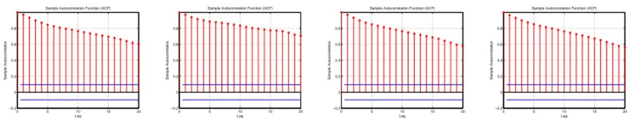
The behaviour of the CDS spreads over time and the autocorrelation function (see
crisis. In fact, according to the Augmented Dickey-Fuller (ADF) test, considering a
first order lag of the autoregressive process and the existence of intercept, trend and
robust standard errors to heteroscedasticity (White), the hypothesis of a unit root
(first order integrated) processes cannot be rejected with 95% confidence (tables 3.5
and 3.6). Therefore, in order to study the default dependency between institutions,
the CDS spreads have to be transformed into stationary variables. Its differentiation
solved the problem for the generality of the cases, as it will be analysed in the next
subsection.
0 5 10 15 20 −0.2 0 0.2 0.4 0.6 0.8 Lag Sample Autocorrelation
Sample Autocorrelation Function (ACF)
0 5 10 15 20 −0.2 0 0.2 0.4 0.6 0.8 Lag Sample Autocorrelation
Sample Autocorrelation Function (ACF)
0 5 10 15 20 −0.2 0 0.2 0.4 0.6 0.8 Lag Sample Autocorrelation
Sample Autocorrelation Function (ACF)
0 5 10 15 20 −0.2 0 0.2 0.4 0.6 0.8 Lag Sample Autocorrelation
Sample Autocorrelation Function (ACF)
Figure 3.2: ACF of CDS spreads before the crisis (bp), for JPMorgan, Goldman Sachs, Bank of America and Citigroup, respectively.
0 5 10 15 20 −0.2 0 0.2 0.4 0.6 0.8 Lag Sample Autocorrelation
Sample Autocorrelation Function (ACF)
0 5 10 15 20 −0.2 0 0.2 0.4 0.6 0.8 Lag Sample Autocorrelation
Sample Autocorrelation Function (ACF)
0 5 10 15 20 −0.2 0 0.2 0.4 0.6 0.8 Lag Sample Autocorrelation
Sample Autocorrelation Function (ACF)
0 5 10 15 20 −0.2 0 0.2 0.4 0.6 0.8 Lag Sample Autocorrelation
Sample Autocorrelation Function (ACF)
Figure 3.3: ACF of CDS spreads during the crisis (bp), for JPMorgan, Goldman Sachs, Bank of America and Citigroup, respectively.
Table 3.5: ADF test for CDS spreads before the crisis.
tstat white critical value 5% critical value 1%
JP Morgan 1.2285 -3.4225 -3.9839
Goldman Sachs 0.2891 -3.4225 -3.9839
Bank of America 0.9197 -3.4225 -3.9839
Citigroup 0.9156 -3.4225 -3.9839
Table 3.6: ADF test for CDS spreads during the crisis.
tstat white critical value 5% critical value 1%
JP Morgan -2.4095 -3.4213 -3.9815
Goldman Sachs -1.3550 -3.4213 -3.9815
Bank of America -1.2060 -3.4213 -3.9815
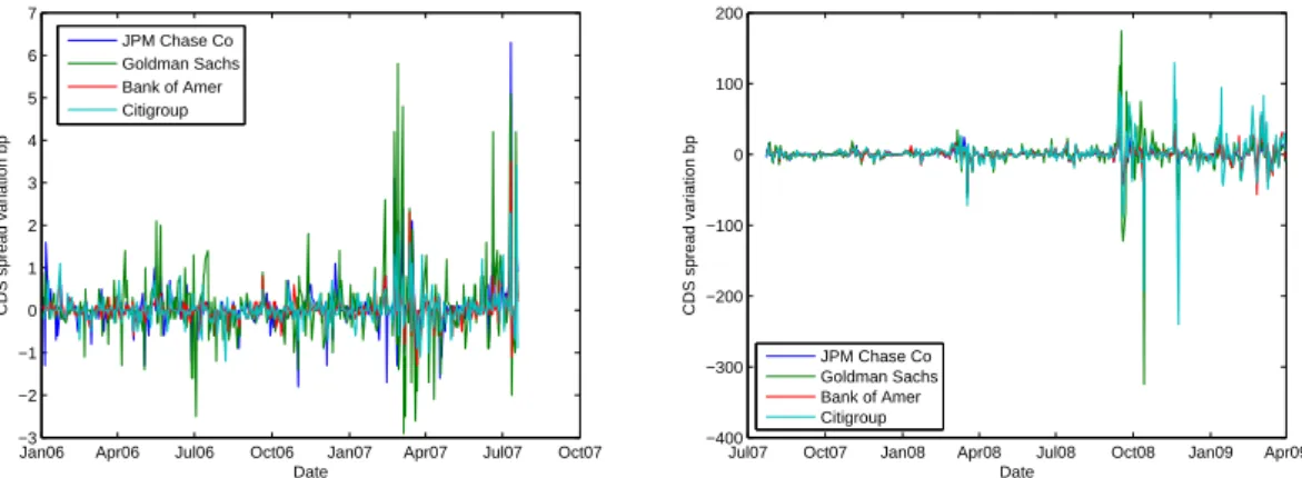
3.1.2 CDS spreads variation
The steps followed in the subsection 3.1.1 are repeated for the first differences of the
CDS spreads, corresponding to the daily discrete changes of the CDS spreads (or
CDS spread variation). The daily variations before the crisis are depicted on the
left-hand side of figure 3.4, ranging between -3 bp and 7bp, while on the right-hand
side of the figure, during the crisis, we observe daily changes higher than 100 bp.
The tails in both periods are very heavy with the skewness changing from positive,
in the first period, to negative, in the second period (tables 3.7 and 3.8), indicating
non-Gaussian behaviour.
Jan06 Apr06 Jul06 Oct06 Jan07 Apr07 Jul07 Oct07 −3
−2 −1 0 1 2 3 4 5 6 7
Date
CDS spread variation bp
JPM Chase Co Goldman Sachs Bank of Amer Citigroup
Jul07 Oct07 Jan08 Apr08 Jul08 Oct08 Jan09 Apr09 −400
−300 −200 −100 0 100 200
Date
CDS spread variation bp
JPM Chase Co Goldman Sachs Bank of Amer Citigroup
Figure 3.4: CDS spreads variation before (left-hand side) and during the crisis (right-hand side).
Table 3.7: Summary statistics of CDS spreads variation before the crisis (bp).
Mean Std Dev Skewness Kurtosis
JP Morgan 0.029 0.56 4.00 45.53
Goldman Sachs 0.067 0.89 2.25 15.73
Bank of America 0.024 0.35 3.50 33.68
Citigroup 0.025 0.41 2.73 20.07
Table 3.8: Summary statistics of CDS spreads variation during the crisis (bp).
Mean Std Dev Skewness Kurtosis
JP Morgan 0.354 8.12 -1.44 22.29
Goldman Sachs 0.502 24.24 -4.61 85.20
Bank of America 0.828 9.82 -0.34 13.11
Citigroup 1.319 22.75 -3.23 47.25
varia-tion of the financial instituvaria-tions increased in the crisis period (tables 3.9 and 3.10) for
the generality of the institutions, with the pairs Goldman Sachs vs Bank of America
and Bank of America vs Citigroup being the exceptions. Before the crisis, the least
correlated pair was JPMorgan vs Citigroup (0.530) and the most correlated was
Bank of America vs Citigroup (0.679). In the crisis period, the highest correlation
occurred between JPMorgan vs Bank of America (0.82) and the smallest (0.555)
belongs to the pair Bank of America vs Goldman Sachs. Note that the correlations
of CDS spreads (tables 3.3 and 3.4) are higher than the respective correlations of
CDS spreads variations, for the generality of the cases. However, recall that the
correlation coefficient is very dependent on the extreme observations. Hence, we
will return to the association level later, when other alternative measures will be
presented within the copula framework.
Table 3.9: Correlation matrix of CDS spreads variation before the crisis (bp).
JP Morgan Goldman Sachs Bank of America Citigroup
JP Morgan 1.000 0.620 0.615 0.530
Goldman Sachs 0.620 1.000 0.585 0.540
Bank of America 0.615 0.585 1.000 0.679
Citigroup 0.530 0.540 0.679 1.000
Table 3.10: Correlation matrix of CDS spreads variation during the crisis (bp).
JP Morgan Goldman Sachs Bank of America Citigroup
JP Morgan 1.000 0.739 0.820 0.744
Goldman Sachs 0.739 1.000 0.555 0.687
Bank of America 0.820 0.555 1.000 0.653
Citigroup 0.744 0.687 0.653 1.000
The stationarity of the CDS spreads variations must be checked for the two
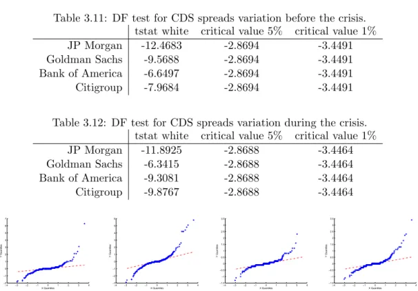
considered periods. According to Dickey Fuller (DF) test, considering intercept and
standard errors robust to heteroscedasticity (White), the hypothesis of a unit root
(first order integrated) processes is rejected with 99% confidence (tables 3.11 and
3.12). Hence, we can proceed with the CDS spreads variation as our interest variable
of default closeness indicator.
As mentioned in tables 3.7 and 3.8, kurtosis is very high for all banks, suggesting