Accounting for Connectivity Uncertainties in Predicting Roadkills:
a Comparative Approach between Path Selection Functions and
Habitat Suitability Models
Francesco Valerio 1,2●Filipe Carvalho3,4●A. Márcia Barbosa2●António Mira1,5●Sara M. Santos1 Received: 9 November 2018 / Accepted: 18 July 2019 / Published online: 1 August 2019
© Springer Science+Business Media, LLC, part of Springer Nature 2019 Abstract
Functional connectivity modeling is increasingly used to predict the best spatial location for over- or underpasses, to mitigate road barrier effects and wildlife roadkills. This tool requires estimation of resistance surfaces, ideally modeled with movement data, which are costly to obtain. An alternative is to use occurrence data within species distribution models to infer movement resistance, although this remains a controversial issue. This study aimed both to compare the performance of resistance surfaces derived from path versus occurrence data in identifying road-crossing locations of a forest carnivore and assess the influence of movement type (daily vs. dispersal) on this performance. Resistance surfaces were built for genet (Genetta genetta) in southern Portugal using path selection functions with telemetry data, and species distribution models with occurrence data. An independent roadkill dataset was used to evaluate the performance of each connectivity model in predicting roadkill locations. The results show that resistance surfaces derived from occurrence data are as suitable in predicting roadkills as path data for daily movements. When dispersal was simulated, the performance of both resistance surfaces was equally good at predicting roadkills. Moreover, contrary to our expectations, we found no significant differences in locations of roadkill predictions between models based on daily movements and models based on dispersal. Our results suggest that species distribution models are a cost-effective tool to build functional connectivity models for road mitigation plans when movement data are not available.
Keywords Movement data● Occurrence data●Telemetry●Species distribution models ●Mitigation ●Dispersal period
Introduction
Linear infrastructures such as highways, roads, railroads, and electric power lines are globally recognized as a major cause of habitat and biodiversity loss (van Der Ree et al.
2011), whose impact is expected to rise considerably in future decades (van der Ree et al. 2015). Roads are responsible for landscape fragmentation, changing animal routes, for direct mortality due to vehicle impact (Coffin
2007; Benítez-López et al.2010), and for jeopardizing the gene-flow exchange in some species (Riley et al. 2006; Bischof et al. 2017). To address such issues, mitigation measures such as over- or underpasses are usually built at specific locations along roads (van Der Ree et al. 2011; Santos et al.2018). The decision about where to locate such measures is often critical, given the uncertainties related to the ecological process to preserve, the scale of analysis, the intrinsic biases (e.g., expert experience, model uncertain-ties) and the existing budgetary limitations (Tulloch et al. * Francesco Valerio
fvalerio@uevora.pt franval.bio@gmail.com
1 Instituto de Ciências Agrárias e Ambientais Mediterrânicas
(ICAAM), University of Évora, Núcleo da Mitra, Edifício Principal, Apartado 94, 7002-554 Évora, Portugal
2 Research Center in Biodiversity and Genetic Resources,
University of Évora (CIBIO/InBIO-UE), Évora, Portugal
3 Research Center in Biodiversity and Genetic Resources (CIBIO/
InBIO), University of Porto, Campus Agrário de Vairão, 4485-661 Vairão, Portugal
4 Department of Zoology and Entomology, School of Biological and
Environmental Sciences, University of Fort Hare, Private Bag X1314, Alice 5700, South Africa
5 Conservation Biology Lab, Department of Biology, University of
Évora, Évora, Portugal
Supplementary information The online version of this article (https:// doi.org/10.1007/s00267-019-01191-6) contains supplementary material, which is available to authorized users.
123456789
0();,:
123456789
2016). Thus, besides the commonly used roadkill hotspots (Bissonette and Cramer 2008; Santos et al. 2011), which may not always be accurate (Santos et al.2015) or avail-able, road ecologists have further considered the benefits of understanding wildlife movements to prioritize resource allocation for mitigation (Allen and Singh2016). Although the coincidence between crossing sites and roadkill sites is not always verified (Neumann et al. 2012), functional connectivity modeling is increasingly used as a tool to predict the best spatial location for animal road-crossing structures by relating functional connectivity with roadkills (Roger et al.2012) as well as road crossing (Cushman et al.
2014).
Functional connectivity is a “species-specific trait that measures the degree by which landscape impedes or facil-itates wildlife movements, and depends on characteristics of the landscape and on species ecology and behavior” (Taylor et al. 1993). Functional connectivity modeling is usually addressed through landscape resistance surface analysis (Zeller et al.2012; Carvalho et al.2016; Correa Ayram et al.
2016). This quantifies “the reluctance of an animal when moving through the landscape and ultimately depicts its physiological cost or mortality risk” (Zeller et al. 2012). Resistance surfaces are thus a crucial step in functional connectivity analysis and can be modeled through numerous approaches (Zeller et al.2012). The simplest is the “expert-based” approach, which consists in one or more experts classifying the resistance of different land use categories (or other landscape elements) based on their experience or on a literature review (Grilo et al. 2011; Wade et al. 2015). However, the above approach has been widely criticized (Wade et al.2015; Correa Ayram et al.2016; McClure et al.
2016), and resistance surfaces are now frequently obtained from model estimations (Pullinger and Johnson2010; Car-valho et al.2016; Ziółkowska et al.2016).
There are multiple criteria to parametrize models for estimating resistance surfaces. Some authors use sequential points in time, i.e., steps (two consecutive points) or paths (e.g., consecutive steps followed during one foraging event) obtained from telemetry data. This allows the development of functions that can be used to predict the probability of animal movement across the study area (Zeller et al.2012), such as path selection functions (PathSFs; e.g., Elliot et al.
2014; Carvalho et al.2016). Another possible approach is to develop species distribution models (SDMs) that use spe-cies occurrence locations (Guisan and Zimmermann2000; Correa Ayram et al. 2016) which can result from direct sightings of animals or other detection methods (tracks, scats, vocalizations, and nests). This approach implies that “the same environmental predictors influence both animal movements and habitat selection” and thus it is assumed that “high habitat suitability values correspond to low landscape resistance values” (Ziółkowska et al. 2016).
Given the types of empirical data required for each modeling approach, occurrence data are usually easier to obtain. However, occurrence data are limited to a specific time and space, meaning that “movement cannot be really measured, but only inferred” (Zeller et al.2012). Sequential points obtained through telemetry are usually preferred over independent occurrence data for deriving resistance surfaces because when they are collected at short time intervals, they reflect the exact pathway taken by an animal (Zeller et al.
2012; Ziółkowska et al.2016). However, path data gathered through telemetry requires a large quantity of information that is more difficult and expensive to obtain, and thus requires more time to convert into a resistance surface (Zeller et al.2012).
Another potential difficulty of path data is that they may include distinct types of movement that can be made during an animal’s lifespan (Coffin2007; van der Grift and van der Ree 2015; Blazquez-Cabrera et al. 2016). There are two main behavioral states: daily movements, made within the home range to fulfill the animals’ primary needs (e.g., foraging, shelter, mating), and dispersal movements to colonize new territories (Pe’er et al. 2011). Some young dispersing animals are known to venture into suboptimal habitats (e.g., extensive open farmland areas), putting their lives at risk, unlike established (resident) animals that use more suitable habitats within their home ranges, such as the Iberian lynx (Blazquez-Cabrera et al.2016) and lions (Elliot et al.2014). Conflating these movement types may produce inaccurate resistance surfaces, and it is thus generally recommended to separate the movement-related behaviors before using them in the paths for connectivity analyses (Zeller et al. 2012; Blazquez-Cabrera et al. 2016). In this context, the use of SDMs may not be sensible, given the uncertainty around which independent occurrence points represent movement within the home range and which represent dispersal movement.
The hypothesis that “animals move in the same way as they select habitat” still remains a matter for discussion (Zeller et al. 2012), focusing on which contexts SDMs can reflect movement models. SDMs can be used at diverse spatial scales, ranging from fine (daily movements or within home range) to broad scales (dispersal) (e.g., Vergara et al.2015). Yet this methodology has been partly contested when applied to assessing functional connectivity. For example, Zió łk-owska et al. (2016) proved that SDMs and step selection function models were equally good at predicting brown bear movements only for small scales, while for road mitigation measures, Blazquez-Cabrera et al. (2016) advocate that SDMs can provide suitable estimates of movement resistance. Road-crossing mitigation structures aim to restore habitat con-nectivity and to reduce the number of roadkills (Bissonette and Cramer 2008; van der Ree et al. 2015). Occurrence of roadkills is commonly driven by species-specific habitat
preferences (Gunson et al. 2011). If we assume a direct relationship between roadkills and habitat features (Gunson et al.2011), this should imply efficient performances in pre-dicting roadkills from habitat suitability models (Roger et al.
2012). It is also commonly assumed in SDMs that opportu-nistically collected fine-scale occurrences (used to fit the models) represent mostly daily movement, as dispersal is an infrequent event in the lifetime of one animal (Cosgrove et al.
2018). Although dispersal is rare, occurring usually once a year, high kill rates have been detected during this biological period (Červinka et al.2015; Carvalho et al.2018). Crossing roads is inherently risky and roads may impair daily move-ment routes through avoidance or barrier effects (Coffin2007; Bissonette and Cramer2008; Cosgrove et al.2018). However, species may be“forced” to cross roads during natal dispersal to reach new territories (Fey et al.2016; Carvalho et al.2018). Consequently, SDM predictions could be significantly biased when validated through high rates of roadkills containing dispersal movements. Daily movements, in fact, should be better related to landscape resistance surfaces than dispersal movements (Hanski 1995; McClure et al. 2016). Thus a transformation function was recently developed for applica-tion on habitat suitability outcomes (Trainor et al. 2013; Keeley et al.2016) so that dispersal resistance surfaces could be better simulated.
To our best knowledge, little is known about the com-parative performance of landscape resistance estimates in pre-dicting animal movements, and there still persists a lack of consensus on which biological data type to use (paths vs. occurrences) (Zeller et al. 2012; Ziółkowska et al. 2016). Quantifying the degree of uncertainty in ecological risk assessment is necessary to provide guidance to decision makers about the efficiency of spatial ecological models (Jaeger2015; Wade et al.2015; Tulloch et al.2016). The understanding of how resistance surfaces can influence the accuracy of road-crossing predictions is a critical issue, given the strong con-servation implications and road agency investments in mitiga-tion measures potentially derived from such analyses. Identification of locations for appropriate application of miti-gation structures that enhance local animal routes is thus of crucial importance for maintaining abundance (Benítez-López et al.2010) and dispersal movements, thereby ensuring gene flow (Riley et al.2006; Cosgrove et al.2018).
Our primary objective was to compare the performance of resistance surfaces derived from (a) path (PathSFs) and (b) occurrence (SDMs) data in predicting road-crossing locations of a forest carnivore. Secondly, we assessed the influence of movement type (daily vs. dispersal) on the above performance, using measures of roadkill prediction accuracy. We hypothesized that (H1) daily resistance sur-faces derived from occurrence data (SDMs) are as suitable in predicting movement (roadkills) as are path data (PathSFs), since suitable habitat characteristics are a key
driver of roadkill patterns (Grilo et al. 2011; Gunson et al.
2011). Consequently, (H2) resistance surfaces derived from simulated dispersal scenarios, using either PathSFs or SDMs, are expected to have lower roadkill predictive per-formance than daily resistance surfaces. However, (H3) predictive performance of resistance surfaces derived from dispersal scenarios can be improved when roadkill data are restricted to the species’ dispersal period.
Medium-sized forest carnivores are highly vulnerable to losses in landscape connectivity and to fragmentation by roads (Grilo et al.2015). Within this group, we selected the genet (Genetta genetta) as a target species because it is a relatively abundant carnivore, specialized in forest habitats and negatively affected by roads (Galantinho and Mira
2009; Carvalho et al. 2014).
We built PathSFs and SDMs that combined environ-mental predictors with either path or occurrence data through a multimodel ensemble of generalized linear mixed models (Duchesne et al. 2010) and generalized linear models (GLMs; Guisan and Zimmermann 2000), respec-tively. The performance of data type (path vs. occurrence) and movement type (daily vs. dispersal) in predicting roadkills was evaluated through the fit of GLMs using discrimination ability and explained variance (Guisan and Zimmermann2000).
Materials and Methods
Study Area
The study area is located in southern Portugal (Fig.1a; 38° 21′48′′–39°00′35′′N, and 8°23′45′′–7°35′08′′W) and cov-ers about 4408 km2. The climate is Mediterranean, domi-nated by mild winters (5.8–12.8 °C) and hot dry summers (16.3–30.2 °C), with a mean annual rainfall of 609.4 mm, falling chiefly from October to March (IPMA 2016). The area is covered mostly by Mediterranean cork/holm oak woodland, with varying tree cover and (open) agricultural areas in approximately equal proportions, lying in a smooth undulating (<420 m a.s.l.) landscape. The area is crossed by several roads, including one highway, and some national and regional roads. For the present study, 102 km of national roads (EN114, EN18, and EN4) were monitored for roadkills of vertebrates (Fig.1). A further description of the study area is provided in Carvalho et al. (2016).
Modeling Procedure
We summarize all modeling steps in a flow chart, from predictor extraction and model settings to movement types used for roadkill predictions (Fig. 2), and we detail below the analytical procedures.
Step (a) Data Acquisition
Genet data
The movement data regarding the study area were obtained within a previous study conducted between 2010 and 2012 (Carvalho et al.2016). The study included telemetry records of 22 resident animals within their home ranges, corre-sponding to a total of 2850 consecutive location records taken at about half-hour intervals, which produced 198 time-independent paths (separated by more than 60 min). For each observed path, nine random paths were generated (Carvalho et al. 2016). We also gathered data on species distribution from the UBC database (Conservation Biology Unit, University of Évora), which included both occur-rences of the genet in the study area, and roadkill locations from 2005 to 2016 (Fig. 2a). These data included 1203 occurrence records with potential to be used in the SDMs. To avoid spatially clustered occurrence patterns and mini-mize spatial auto-correlation, we applied a rarefaction pro-cedure (Kramer-Schadt et al.2013). In this process, only occurrences that are at least 1000 m away from each other (ca 300 ha buffer, an approximation to the mean home range size of this species, Santos-Reis et al.2005; Carvalho et al.
2014) were kept for further analyses (Fig. 2a). Thus, 175 records of genet occurrence werefinally included in SDMs.
We then defined an equal proportion of pseudo-absences (n= 175; Fig.2a) assigned randomly from the extent of the study area (Barbet-Massin et al.2012), excluding the non-rarefied occurrence cells.
Genet roadkills consisted of 77 locations of genet car-casses identified on monitored paved roads (Fig. 1a). Sur-veys were done previously by one experienced observer driving at 20–40 km/h. All genet carcasses, once detected, were registered with a GPS and removed from the road to avoid double counting (e.g., Santos et al. 2013).
Environmental predictors
SDMs predictors and the analysis protocol were as similar as possible to those used in previous PathSFs models (Carvalho et al. 2016) to allow comparability of the resis-tance surface performance (Table 1). We prepared a set of landscape predictors at 100-m resolution using CORINE Land Cover data (Guiomar et al.2009) to characterize paths (observed and random) and occurrence points (Fig. 2a). These include landscape composition (percent cover of oak forests, open agricultural land, and urban areas), landscape configuration (mean forest patch size, forest edge density, and tree canopy openness), and distance to important landscape resources (forests, riparian habitats, and water bodies; Table 1; Carvalho et al. 2016). The predictors Fig. 1 a Location of the study
area in Portugal. b Spatial distribution of genet roadkills and monitored roads in the study area, overlaid on a layer with the main land uses
concerning landscape composition and configuration were measured for two spatial scales (McGarigal et al. 2016): within a 100 m buffer (immediate surroundings perceived by the animal when following a path) and within a 500 m buffer (the larger area available to the animal when making movement decisions). The distance predictors were scale independent (see Carvalho et al.2016for details). We used round moving windows (McGarigal et al. 2012) for the landscape class-level metrics, and focal foci to assess optimal neighborhood scale (Holland and Yang 2016) for the canopy openness predictor.
Step (b) Model Building
Prior to model building, predictors were evaluated for nor-mality and the effect of extreme values was softened through angular or logarithmic transformations, and standardized to zero mean and unit variance to allow comparability of their effects (see Carvalho et al.2016). The degree of collinearity among candidate predictors was evaluated through a pairwise Pearson correlation test. For pairs with |r| > 0.7, only the vari-able with the highest biological meaning, based on previous studies of the species, was retained (see Carvalho et al.2016). Fig. 2 Flow chart representing model building and comparisons of roadkill predictions between path selection functions (PathSFs) and species distribution models (SDMs), accounting for both movement types (daily and dispersal). See the main text for details
Because path and occurrence data have different spatial properties, the modeling approaches were also slightly dif-ferent (Fig. 2b). PathSFs were built with mixed effects conditional logistic regression, to account for stratification of random paths and inter-individual heterogeneity in path selection (Duchesne et al.2010; Carvalho et al.2016). For SDMs, GLMs with binomial error distribution and a logistic link function were applied (Guisan and Zimmermann2000). Both approaches compared landscape characteristics of observed paths (or occurrences) with random paths (or pseudo-absences).
Predictor screening in both approaches was conducted with univariate analysis based on mixed models or GLMs, respectively. We compared each single-predictor model with a null model using the Akaike information criterion (AIC; Burnham and Anderson2002). Only predictors pro-ducing models with strong support (ΔAIC > 10) were selected for the subsequent multivariate analyses (Table1). We built PathSFs and SDMs multivariate models with all possible combinations of the selected predictors (including the null and the full models), and used a multimodel inference procedure (Burnham and Anderson2002) to rank the models based on their Akaike weights (wi). The average
parameters and unconditional standard errors (SEs) were estimated for the set of models that differed by less than four in their AIC from the most supported model (Burnham and Anderson 2002). The model coefficient of a predictor was considered statistically significant if estimates of its 95% confidence interval did not include zero. The con-tribution of each predictor was based on the sum of Akaike weights for the models in which that predictor was con-tained (w+) and on the magnitude of the average model coefficient. We evaluated model performance through the amount of explained deviance (D-squared; Guisan and Zimmermann2000) and discrimination ability was assessed by the area under the receiver operating characteristic (ROC) curve (AUC) (Fielding and Bell1997; Swets1988). The averaged PathSFs and SDMs model predictions were applied to estimate movement probability on a grid of 100-m scale (Carvalho et al.2016).
Step (c) Roadkill Predictions: Habitat and Dispersal
Resistance Surface Performances
We derived additional movement probability maps (for PathSFs and SDMs) in order to evaluate the optimal Table 1 Summary univariate statistics of predictors used for SDMs models, with indication of scale used, abbreviation, mean, and SD values for sites with genet occurrence and pseudo-absence
Predictor Scale (m) Abbreviation Genet occurrences Genet random pseudo-absences
ΔAIC
Mean ± SD Range Mean ± SD Range
Landscape composition 100
Forest areas (%) PLAND_FOR 60.97 ± 37.23 0–100 36.93 ± 39.94 0–100 55.63
Agriculture areas (%) PLAND_AGR 31.59 ± 34.45 0–100 49.07 ± 40.17 0–100 41.11
Urban areas (%) PLAND_URB 0.61 ± 2.96 0–28.43 1.64 ± 7.82 0–80.47 25.07
Landscape composition 500
Forest areas (%) PLAND_FOR 57.58 ± 30.23 0–100 38.32 ± 32.47 0–99.75 52.94 Agriculture areas (%) PLAND_AGR 34.83 ± 27.57 0–98.18 48.93 ± 32.25 0–100 42.79
Urban areas (%) PLAND_URB 0.80 ± 2.44 0–17.01 1.20 ± 6.017 0–68.94 22.99
Landscape configuration 100
Canopy openness (m) Canopy 71.82 ± 17.65 19.67–91 81.61 ± 12.19 33.38–91 54.8 Forest edge density (m/ha) ED_FOR 36.38 ± 34.9 0–79.28 26.01 ± 32.21 0–112.93 31.37
Forest patch size (ha) AREA_MN_FOR 3.03 ± 1.87 0–5 1.84 ± 1.99 0–5 57.43
Landscape configuration 500
Canopy openness (m) Canopy 0.61 ± 0.11 0.23–0.7 0.67 ± 0.08 0.28–0.81 53.7 Forest edge density (m/ha) ED_FOR 33.42 ± 18.55 0–114.73 27.85 ± 21.39 0–84.24 38.6 Forest patch size (ha) AREA_MN_FOR 38.99 ± 28.35 0–81 24.25 ± 25.70 0–80.8 53.17 Distance to habitats –
Distance to forests (m) Euc_Dist_FOR 79.22 ± 138.02 0–903 256.85 ± 351.2 0–2309 59.79 Distance to a riparian habitats (m) Euc_Dist_RIP 387.18 ± 346.69 6–2129 589.66 ± 436.26 38–2476 54.67 Distance to water (m) Euc_Dist_WAT 1213.97 ± 776.9 61–3671 1272.10 ± 961.32 0–5397 22.85 Predictors are grouped into three categories (landscape composition, configuration, and distance to habitats). The same three landscape class-level metrics used on PathSFs analysis were also calculated for SDMs and regarded the same land cover types. Land cover types considered were as follows: FOR forest areas, AGR agriculture areas, and URB urban areas
neighborhood scale (Cushman et al. 2014; Holland and Yang 2016). For each pixel, we extracted movement probability values fromfive neighbor distances (0, 50, 100, 200, and 300 m; Fig. 2c). We applied a normalization procedure to guarantee that pixel values of each movement probability map remained within the range of 0–1. Each of these movement probability maps was transformed into a resistance map by linearly inverting the probability values (Wade et al.2015).
To test H1 (PathSFs and SDMs produce equally good habitat-based resistance surfaces for predicting roadkills), we compared the performance of each type of resistance surface in explaining the occurrence pattern of roadkills by using binomial GLMs. In order to apply these models, roadkill pseudo-absences were randomly generated (with a 50% prevalence, i.e., the same number of observed pre-sences and pseudo-abpre-sences) along the monitored roads. Accordingly, we defined three datasets (presence/absence of roadkills) that vary in the minimum distance (MD) between an absence and a roadkill location: 100, 500, and 1000 m. This procedure intends to minimize false-negative bias (Barbet-Massin et al.2012; Fielding and Bell 1997). Each MD roadkill dataset (MD100, MD500, and MD1000) was used as the response variable in univariate GLMs, and each of the five defined resistance surfaces were used as pre-dictors (resulting in combinations of 15 GLMs per data type model; Fig.2c). Model fit was verified through the AUC (Fielding and Bell1997), the amount of explained deviance (Guisan and Zimmermann 2000), AIC and a ΔAIC com-parison between the best-performing model of PathSFs or SDMs vs the of PathSFs or SDMs (for each MD). We used a ΔAIC threshold of four to evaluate the magnitude of support between models (Burnham and Anderson 2002; Carvalho et al.2016; Salgueiro et al.2018). Results were averaged across ten replicates run on the training (75%) and randomly chosen test (25%) datasets. The performance differences of PathSFs and SDMs in predicting roadkills (H1) was assessed through a DeLong test that compares ROC curves between different models (1000 permutations). Statistical divergence between curves was set to p < 0.05.
In order to test the working hypotheses concerning dis-persal movements (H2 and H3), we obtained simulated dispersal resistance maps by applying a negative exponen-tial transformation function (Keeley et al. 2016) on the previously evaluated PathSFs and SDMs best resistance surfaces models in H1 (Fig.2c). When landscape resistance is estimated from SDMs, it is usually assumed to be a negative linear function of suitability; in other words, the resistance decreases at a constant rate as suitability increases (Keeley et al. 2016). Using an exponential transformation means that larger portions of the landscape will be coded as low resistance to movement (Keeley et al. 2016), thus approaching more generalist habitat choices during
dispersal events. We used as an exponential transformation function the following equation: R= 100 − 99 × ((1 − exp (−c × h))/(1 − exp(−c))), in which R is resistance, h is probability of movement taken from PathSFs or SDMs models, and c is the degree of the function corresponding to 0.25, 0.5, 1, 2, 4, or 8 (Fig. 2c). For each of the seven transformations, resistance is minimum when probability of movement is maximum. At c= 0.25, the relationship is almost linear, being equivalent to the previous daily resis-tance surface. As c increases, resisresis-tance values change from a linear towards an exponential decay function, with resis-tance to movement decreasing more rapidly (and reaching the asymptote sooner) with increasing habitat suitability (Keeley et al. 2016). Thus, we calculated six dispersal resistance surfaces for each data type model (PathSFs and SDMs). Simulated dispersal resistance maps were validated against roadkills using GLMs, as in previous analyses. However, for hypotheses H2 and H3, we used only one MD dataset (that with the best performance in previous analysis; Fig. 2c). To determine whether roadkill identification per-formance significantly decreased (H2) or improved (H3), we used the ΔAIC by comparing the performance of each model vs the best model (for PathSFs and SDMs separately).
Similar analyses were used to test H2 and H3. However, for H2, all-year-round roadkill records were included, while for H3 roadkill data were restricted to the dispersal period of the genets (September–March; Larivière and Calzada2001). Because such movements are more common among juve-niles or subadults (Fey et al.2016; Carvalho et al.2018), we further excluded all identified road-killed adults (animals with a lower probability of being in dispersal) from H3 testing.
Analyses were conducted with R v.3.3.1 (R Develop-ment Core Team. 2016), QGIS v2.6 (Quantum GIS Development Team 2015), and Fragstats v4.2 (McGarigal et al. 2012). The following R packages were applied: “spThin” (Aiello-Lammens et al. 2015),“raster” (Hijmans
2016),“MuMIn” (Barton2016),“ModEvA” (Barbosa et al.
2016), and“pROC” (Robin et al.2011).
Results
General Results on SDMs
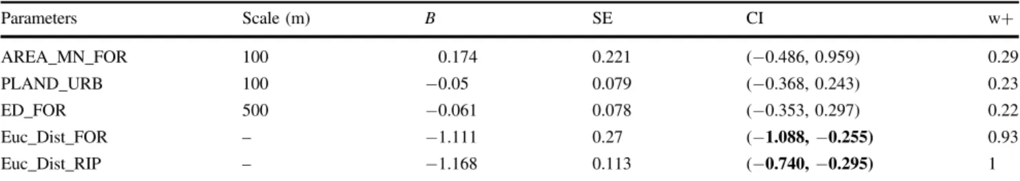
The SDMs results were in accordance with those of pre-viously built PathSFs models. The average SDMs model included five predictors. Genet presence is more likely in areas close to riparian and forest habitats, as these predictors have high support in the average model (w +> 0.90; Table2). In addition, areas with large forest pat-ches, reduced urban presence, and reduced forest edge
density also contribute to the increase in probability of species presence (Table2). This model showed a D-squared value of 0.124 and resulted in a good discrimination ability (AUC= 0.7), which is close to PathSFs results (R-squaredPathSFs= 0.33, AUCPathSFs= 0.8; Carvalho et al.
2016).
Resistance Surfaces for Prediction of Daily
Movements (H1)
For both types of models (PathSFs and SDMs) we found that model performance in explaining roadkill sites (AUC, D-squared, and AIC) increased with increasing MD Table 2 Summarized results for the averaged SDMs model: standardized regression coefficients (B), unconditional standard errors (SEs), 95% confidence intervals of coefficient estimates (CI), and selection probability (w+) for each predictor in SDMs
Parameters Scale (m) B SE CI w+ AREA_MN_FOR 100 0.174 0.221 (−0.486, 0.959) 0.29 PLAND_URB 100 −0.05 0.079 (−0.368, 0.243) 0.23 ED_FOR 500 −0.061 0.078 (−0.353, 0.297) 0.22 Euc_Dist_FOR – −1.111 0.27 (−1.088, −0.255) 0.93 Euc_Dist_RIP – −1.168 0.113 (−0.740, −0.295) 1
Coefficient estimates whose 95%CI exclude zero are in bold. The PathSFs average model results showed similar predictors having high support (forest predictors and distance to riparian habitats) and are presented in Carvalho et al. (2016). Original names and associated calculated metrics of the abbreviation parameters are referred in Table1
Fig. 3 Performance comparison results of path data (PathSFs) and occurrence data (SDMs) in predicting genet roadkills using all calcu-lated neighbor distances (0, 50, 100, 200, and 300 m) and roadkill dataset (MD100–MD1000): a Area under the ROC curve (AUC);
b amount of explained deviance (D-squared); c Akaike’s information criterion (AIC); and d comparison of ROC curves (DeLong test) and p-value similarity threshold (horizontal black line)
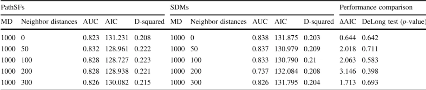
datasets, with the best models corresponding to MD1000 dataset (Fig. 3a–c). These models had the highest AUC values and explained deviance (AUC > 0.80; D-squared > 0.15) and presented the lowest AIC scores (Fig.3a–c).
When comparing the performance of each type of resistance surface in explaining roadkill patterns, we found that SDMs performed similarly (AUC and D-squared) in explaining roadkill data when compared with PathSFs, a result consistent through all roadkill datasets (MD100–MD1000; Fig. 3a, b). Moreover, the differences in AIC and in ROC curves were not statistically significant for neither datasets (ΔAIC < 4; p values of DeLong tests > 0.05; Fig.3c, d; Table3). The similarities between SDMs and PathSFs resistance maps are shown in Figs4a–b and5. We thus conclude that the resistance surfaces derived from occurrence data (SDMs) are as suitable in predicting roadkills as are path data (PathSFs), thereby supporting hypothesis H1.
Resistance Surfaces for Prediction of Dispersal
Movements (H2 and H3)
We also compared the performance of models including dispersal resistance surfaces in explaining a complete dataset (all-year-round roadkills; H2) and a dispersal-only dataset (H3). The dispersal resistance maps (e.g., c= 4 and c = 8) are presented in Fig. 5 for both models and their similarities are apparent.
When using the complete roadkill dataset (H2), we found that ΔAIC scores showed decreasing performance from daily (c= 0.25) to dispersal movements (0.5 < c < 8; Fig.
4a). However, this AIC variation is <4, meaning that models do not statistically differ and thus rejecting H2. The scenario is similar for the dataset including only roadkills within the dispersal period (ΔAIC < 4), and H3 is also not supported (Fig.4b). For further details on H2 and H3 results see Table S2.
Discussion
Connectivity models often suffer from lack of validation with independent data and are therefore subject to uncer-tainty (Zeller et al.2012; Wade et al.2015; Correa Ayram et al. 2016). We used genet roadkill locations to validate landscape connectivity models built with“real movement” and “occurrence” data. Moreover, we compared the per-formance of models using daily movements with models using inferred dispersal, as they correspond to different life-events associated with individual survival and long-term population persistence. Juvenile as well as subadult are the most road-killed age classes for the genet and causalities are higher during the dispersal period (Carvalho et al. 2018). Both these facts suggest that dispersal is a critical event explaining temporal patterns of genet roadkills.
Our spatial analysis confirmed that landscape character-istics can be a valuable proxy of functional connectivity, and wherever roads approach or bisect suitable habitats, they are more prone to be crossed by animals, as maintained by others (Grilo et al.2011; D’Amico et al.2015; Kari and Zimmermann 2015). We found a relationship of roadkills with connectivity maps derived from SDMs, which is consistent with previous studies (Roger et al.2012) and also with maps derived from PathSFs, for which we have no knowledge in the literature. In particular, for both model types, the substantially improved performance with increasing MD distances seems to be related to a decrease in false absence error rates, resulting in a smaller negative effect of false absences (Fielding and Bell1997). There is a growing body of scientific literature that suggests caution be taken when accounting for false absence bias (Barbet-Massin et al. 2012) and we highlighted its importance. Indeed, this is an underestimated issue in road ecology that can compromise the reliability of prediction models (Santos et al.2018).
Table 3 Data type models (PathSFs and SDMs) specific results regarding all the focal foci associated to the most performant MD (MD1000)
PathSFs SDMs Performance comparison
MD Neighbor distances AUC AIC D-squared MD Neighbor distances AUC AIC D-squared ΔAIC DeLong test (p-value)
1000 0 0.823 131.231 0.208 1000 0 0.838 131.875 0.203 0.644 0.642
1000 50 0.832 128.961 0.222 1000 50 0.837 130.979 0.209 2.018 0.711
1000 100 0.828 128.727 0.223 1000 100 0.833 130.790 0.21 2.063 0.583 1000 200 0.828 128.938 0.221 1000 200 0.737 132.084 0.208 3.146 0.398 1000 300 0.826 130.082 0.215 1000 300 0.826 131.795 0.204 1.713 0.693
Accuracy scores were based on AUC, D-squared, AIC,ΔAIC, and p-values of the DeLong test. For further details regarding all the MD results see Table S1
Comparison of Model Performance
The similarity in performance of roadkill predictions between SDMs and PathSFs suggests that connectivity models of both types are determined by similar predicted patterns and supports the hypothesis that movement is most facilitated in suitable habitats. For the genet, a higher probability of movement (and roadkills) is expected within or in the proximity of forest habitats, which often contain
more stable and abundant resources (Carvalho et al. 2016) and thereby can be translated into lower variability of inter movement decisions (Duchesne et al. 2010). Thus, simple models based on occurrence data may be as able to deter-mine how environmental parameters affect movements as more complex models based on path data. Moreover, con-sidering the link between scales and the ecological process under investigation (Holland and Yang 2016; McGarigal et al. 2016), PathSFs and SDMs results may have been converged given the scale-dependent relationship of road-kills with movement type and land-use patterns. Speci fi-cally, scales within species’ home range are adequate to capture landscape characteristics that should be taken into account when applying mitigation measures (Gunson et al.
2011;Červinka et al.2015), thereby representing a feasible “scale of management” (Allen and Singh 2016; Cosgrove et al.2018).
Besides, when we compared roadkill prediction perfor-mance regarding the impact of behavior, whether daily movements or dispersal, the latter responded similarly, meaning that models based on daily movements can be as good as those based on dispersal, when choosing the loca-tions for roadkill mitigation measures. One possible expla-nation for the lack of support for H2 might stem from a potential behavioral contamination, due to inclusion of the nondispersal period in the initial analysis. However, in a further analysis, dispersal-based prediction of roadkills did not improve when using only data for the dispersal period, contrary to expectations, thus also leading to the rejection of H3. Interpretation of such results may not be straightforward and needs prudence because terrestrial carnivore dispersing strategies may be influenced by individual variability in movement decisions (Oriol-Cotterill et al.2015), which may be triggered as a mechanism of antipredator response toward a human-caused mortality risk (Jacobson et al.2016). Such dispersing plasticity may include juveniles that adopt movements associated normally to adults (e.g., throughout favorable habitats). For example, this often happens when juvenile offspring, with no prior knowledge of the land-scape, are accompanied by their more sensitive-to-risk mothers in their early exploratory movements (Beier 1995; Oriol-Cotterill et al. 2015). Moreover, riparian habitats, which had the most pronounced effects for both data type models (Carvalho et al. 2016), are often used as corridors during dispersal movements and simultaneously provide optimal residence habitat for multiple mesocarnivores spe-cies including genet (Carvalho et al.2016; Grilo et al.2016). On the other hand, adult genets may undertake extra-territorial habitat movements across supposedly avoided roads (Carvalho et al. 2018) which might contribute to reducing potential bias effect due to the small number of identified dispersing juveniles in the datasets. Although road avoidance is likely to exclude carnivore road-crossing Fig. 4 Comparison of performance results (ΔAIC) between path data
(PathSFs) and occurrence data (SDMs) in predicting genet roadkills for daily movement (c= 0.25) and for simulated dispersal movement (0.5≤ c ≤ 8); a considering all roadkills and b considering only road-kills within the dispersal period. Horizontal black lines indicate the significance threshold (ΔAIC = 4), meaning that differences under the line are interpreted as nonsignificant
events, increases in mortality rates have been documented following decreases in traffic volume (Alexander et al.2005) or after rainy nights when road culverts become flooded (Craveiro et al.2019). Thus, roads may occasionally act as a filter rather than being an absolute barrier (Jacobson et al.
2016; Ceia-Hasse et al.2018).
Wide-ranging animals, such as carnivores, may encounter roads during different types of movements and behaviors (Ceia-Hasse et al.2018), as outlined above. Once again, this issue is unlikely to be tackled in most road ecology studies, and when we accounted for it, the inter-pretation of our results is that the biasing behavior toward our employed roadkill datasets (global and dispersal) was not capable of significantly undermining the habitat suitability-roadkill relationship. Globally, our results rein-force the importance of roadkill mitigation measures that allow for the promotion of movements associated with different ecological processes, as explained below.
Management Implications
Functional connectivity models are generally more efficient when they include movement data. However, despite the
advantages of pathway data, this information is costly to obtain in terms of time, manpower and money, and con-servation actions are constantly faced with limited funding, which plays a paramount role when choosing the final solution (e.g., Santos et al. 2015). Placement of mitigation structures can be optimized by using models that draw on more easily available data, such as SDMs, because such models may adequately reflect the interactions between species and environment across spatial scales (Guisan et al.
2013). The SDMs cost-benefit tradeoff is enhanced when we take into account the growing demand for multiple species assessments (Khosravi et al.2018), as the collection of a comprehensive multispecies pathway dataset is ham-pered by limited budgets. We therefore support such an application, in the context addressed herein, for other spe-cies and with different behaviors or life stages, as long as the SDMs modeling framework is explicit and justified within the context of conservation purposes (Guisan et al.
2013; Tulloch et al.2016).
Conservation can operate at different scales, and previous studies required the selection of a proper planning scale that would integrate a pattern-process linkage associated with roadkills (Ims1995; Kari and Zimmermann2015; Tulloch Fig. 5 Comparison of resistance maps between PathSFs and SDMs for
the movement of genets (higher resistance values in black, lower resistance values in white) overlaid with roadkills sites; a PathSFs daily movement scenario (c= 0.25); b PathSFs intermediate dispersal
movement scenario (c= 4); c PathSFs high-level dispersal movement scenario (c= 8); d SDMs daily movement scenario (c = 0.25); e SDMs intermediate movement scenario (c= 4); f SDMs high-level dispersal movement scenario (c= 8)
et al. 2016; Cosgrove et al. 2018). Indeed, the type of mitigation should depend on both the target species and movement to promote (Smith et al.2015; van der Grift and van der Ree 2015; Allen and Singh 2016). The analysis showed that daily and dispersal movements are simulta-neously accounted for by SDMs. This fact, together with their simplicity (compared with PathSFs), makes them use-ful tools to guide the installation of road mitigation measures targeting both dispersers and residents. SDMs may be useful to support conservation managers as they can identify sui-table locations (e.g., wherever roads intersect high con-nectivity areas) for roadkill mitigation measures (e.g., fauna passages, culvert adaptations, etc.), ensuring the accom-plishment of daily routines associated with feeding, protec-tion from predators and reproducprotec-tion, and simultaneously promoting the geneflow, associated with dispersal, which is critical for long-term population persistence (van Der Ree et al.2011).
Nevertheless, distinguishing between resident experi-enced adults and subadult dispersers may be important as long corridors linking distant suitable habitat patches might be mostly used by few dispersing individuals. Conse-quently, it should be noted that although locally placed crossing structures might be successful in ensuring the gene flow between subpopulations (Sawaya et al.2014; Carvalho et al. 2018), higher scales of planning like regional/inter-national coordinated strategies are still needed for the pro-motion of large ecological networks and inter-population geneflow (van Der Ree et al. 2011; Jaeger 2015). Ecolo-gical corridors applied across wide study areas (e.g., regional scales or higher) normally better rely on dispersal resistance surfaces, since when constructed through habitat suitability or movements within the home range, such cor-ridors may greatly overestimate resistance to movement (Blazquez-Cabrera et al.2016; Ziółkowska et al.2016). In such contexts, the use of a negative exponential transfor-mation function (Trainor et al. 2013; Keeley et al. 2016) may be more relevant as the generally lower resistance to movements renders distant patches more reachable by a few dispersers, thereby increasing the confidence of corridor placement (e.g., Khosravi et al.2018). Lastly, we argue that these corridors might be likely to benefit other dispersing forest mammal species, given the similar dimension of home range to the species we examined, which in turn can be translated into a capability of similar dispersal distances or suchlike (Bowman et al.2002).
Conclusions
In this paper, our spatial analysis showed a consensus of two comprehensive frameworks to identify road-crossing sites by a forest carnivore. We specifically demonstrated
that, regardless of the model complexity (occurrence or paths), landscape elements characterizing species habitat may be a helpful proxy of functional connectivity in explaining roadkills and therefore in allocating management resources. Our results presented herein afforded valuable insights to solve uncertainties in predicting roadkills regarding some of the most widely used data type models, providing support for the use of SDMs. Moreover, we demonstrated that our models simultaneously consider daily movements and dis-persal associated to roadkills, emphasizing the reliability of both SDMs and PathSFs in targeting both dispersers and residents at the local scale. We suggest that SDMs are a viable option to build resistance surfaces for functional connectivity models either in single species or multispecies projects, and with similar results for different life stages and behaviors. This is especially important for large scale con-nectivity assessments, such as multispecies defragmentation plans of high road-density landscapes (Santini et al.2016). Acknowledgements FV is grateful to Marco Basile and Sabrina Mazzoni for their suggestions on earlier versions of the manuscript, and also to Mark Walter for the final English revision. The authors would also like to thank the MOVE team for road survey data col-lection and Rafael Carvalho for the genet radio tracking data collec-tion. We also thank two anonymous reviewers for their help in improving this paper. FV was supported by a PhD fellowship, while SMS, AMB and FC by postdoctoral contracts, which were all funded by Fundação para a Ciência e a Tecnologia (SFRH/BD/122854/2016, SFRH/BPD/70124/2010, IF/00266/2013/CP1168/CT0001 and SFRH/ BPD/115228/2016, respectively). We also received support from the projects LIFE LINES (LIFE14 NAT/PT/00108) and POPCONNECT (PTDC/AAG-MAA/0372/2014).
Funding FV was supported by a PhD fellowship, while SMS, AMB, and FC by postdoctoral contracts, which were all funded by Fundação para a Ciência e a Tecnologia (SFRH/BD/122854/2016, SFRH/BPD/ 70124/2010, IF/00266/2013/CP1168/CT0001, and SFRH/BPD/ 115228/2016, respectively). We also received support from the pro-jects LIFE LINES (LIFE14 NAT/PT/00108) and POPCONNECT (PTDC/AAG-MAA/0372/2014).
Compliance with Ethical Standards
Conflict of Interest The authors declare that they have no conflict of interest.
Publisher’s note: Springer Nature remains neutral with regard to jurisdictional claims in published maps and institutional affiliations.
References
Aiello-Lammens ME, Boria RA, Radosavljevic A, et al. (2015) spThin: an R package for spatial thinning of species occurrence records for use in ecological niche models. Ecography. https:// doi.org/10.1111/ecog.01132
Alexander SM, Waters NM, Paquet PC (2005) Traffic volume and highway permeability for a mammalian community in the Canadian Rocky Mountains. Can Geogr 49:321–331.https://doi. org/10.1111/j.0008-3658.2005.00099.x
Allen AM, Singh NJ (2016) Linking movement ecology with wildlife management and conservation. Front Ecol Evol 3:155.https://doi. org/10.3389/fevo.2015.00155
Barbet-Massin M, Jiguet F, Albert CH, Thuiller W (2012) Selecting pseudo-absences for species distribution models: how, where and how many?. Methods Ecol Evol 3:327–338.https://doi.org/10. 1111/j.2041-210×.2011.00172.x
Barbosa AM, Brown JA, Jimenez-Valverde A, Real R (2016) mod-EvA: model evaluation and analysis. R package version 1.3.2.
https://CRAN.R-project.org/package=modEvA
Barton K (2016) MuMIn: multi-model inference. R package version 1.15.6.https://CRAN.R-project.org/package=MuMIn
Beier P (1995) Dispersal of juvenile cougars in fragmented habitat. J Wildl Manag 59:228–237.https://doi.org/10.2307/3808935
Benítez-López A, Alkemade R, Verweij PA (2010) The impacts of roads and other infrastructure on mammal and bird populations: a meta-analysis. Biol Conserv 143:1307–1316.https://doi.org/10. 1016/j.biocon.2010.02.009
Bischof R, Steyaert SMJG, Kindberg J (2017) Caught in the mesh: roads and their network-scale impediment to animal movement. Ecography 40:1369–1380.https://doi.org/10.1111/ecog.02801
Bissonette JA, Cramer P (2008) Evaluation of the use and effective-ness of wildlife crossings. NCHRP Report No. 615, National Cooperative Research Program, Transportation Research Board of the National Academies, Washington, D.C., p 161
Blazquez-Cabrera S, Gastón A, Beier P et al. (2016) Influence of separating home range and dispersal movements on characteriz-ing corridors and effective distances. Landsc Ecol 31:2355–2366.
https://doi.org/10.1007/s10980-016-0407-5
Bowman J, Jaeger JAG, Fahrig L (2002) Dispersal distance of mam-mals is proportional to home range size JSTOR. 83:2049–2055.
https://doi.org/10.1002/smj.192
Burnham KP, Anderson DR (2002) Model selection and multimodel inference: a practical information-theoretic approach. Springer, New York
Carvalho F, Carvalho R, Mira A, Beja P (2014) Use of tree hollows by a Mediterranean forest carnivore. For Ecol Manag 315:54–62.
https://doi.org/10.1016/j.foreco.2013.12.013
Carvalho F, Carvalho R, Mira A, Beja P (2016) Assessing landscape functional connectivity in a forest carnivore using path selection functions. Landsc Ecol 31:1021–1036. https://doi.org/10.1007/ s10980-015-0326-x
Carvalho F, Lourenço A, Carvalho R et al. (2018) The effects of a motorway on movement behaviour and gene flow in a forest carnivore: Joint evidence from road mortality, radio tracking and genetics. Landsc Urban Plan 178:217–227. https://doi.org/10. 1016/j.landurbplan.796
Ceia-Hasse A, Navarro LM, Borda-de-Água L, Pereira HM (2018) Population persistence in landscapes fragmented by roads: disen-tangling isolation, mortality, and the effect of dispersal. Ecol Model 375:45–53.https://doi.org/10.1016/j.ecolmodel.2018.01.021
Červinka J, Riegert J, Grill S, Šálek M (2015) Large-scale evaluation of carnivore road mortality: the effect of landscape and local scale characteristics. Mamm Res 60:233–243.https://doi.org/10.1007/ s13364-015-0226-0
Coffin AW (2007) From roadkill to road ecology: a review of the ecological effects of roads. J Transp Geogr 15:396–406.https:// doi.org/10.1016/j.jtrangeo.2006.11.006
Correa Ayram CA, Mendoza ME, Etter A, Salicrup DRP (2016) Habitat connectivity in biodiversity conservation. Prog Phys Geogr 40:7–37.https://doi.org/10.1177/0309133315598713
Cosgrove AJ, McWhorter TJ, Maron M (2018) Consequences of impediments to animal movements at different scales: a con-ceptual framework and review. Divers Distrib 24:448–459.
https://doi.org/10.1111/ddi.12699
Craveiro J, Bernardino J, Mira A, Vaz PG (2019) Impact of culvert flooding on carnivore crossings. J Environ Manag 231:878–885.
https://doi.org/10.1016/j.jenvman.2018.10.108
Cushman SA, Lewis JS, Landguth EL (2014) Why did the bear cross the road? Comparing the performance of multiple resistance surfaces and connectivity modeling methods. Diversity 6:844–854.https://doi.org/10.3390/d6040844
D’Amico M, Román J, de los Reyes L, Revilla E (2015) Vertebrate road-kill patterns in Mediterranean habitats: who, when and where. Biol Conserv 191:234–242. https://doi.org/10.1016/j. biocon.2015.06.010
Duchesne T, Fortin D, Courbin N (2010) Mixed conditional logistic regression for habitat selection studies. J Anim Ecol 79:548–555.
https://doi.org/10.1111/j.1365-2656.2010.01670.x
Elliot NB, Cushman SA, Macdonald DW, Loveridge AJ (2014) The devil is in the dispersers: predictions of landscape connectivity change with demography. J Appl Ecol 51:1169–1178.https://doi. org/10.1111/1365-2664.12282
Fey K, Hämäläinen S, Selonen V (2016) Roads are no barrier for dispersing red squirrels in an urban environment. Behav Ecol 27:741–747.https://doi.org/10.1093/beheco/arv215
Fielding AH, Bell JF (1997) A review of methods for the assessment of prediction errors in conservation presence / absence models. Environ Conserv 24:38–49.https://doi.org/10.1017/S0376892997000088
Galantinho A, Mira A (2009) The influence of human, livestock, and ecological features on the occurrence of genet (Genetta genetta): a case study on Mediterranean farmland. Ecol Res 24:671–685.
https://doi.org/10.1007/s11284-008-0538-5
Grilo C, Ascensão F, Santos-Reis M, Bissonette JA (2011) Do well-connected landscapes promote road-related mortality? Eur J Wildl Res 57:707–716. https://doi.org/10.1007/s10344-010-0478-6
Grilo C, Smith DJ, Klar N (2015) Carnivores: struggling for survival in roaded landscapes. In: Handbook of road ecology. Wiley-Blackwell, pp 300–312.https://doi.org/10.1002/9781118568170. ch35
Grilo F, Ferreira E, Alcobia S et al. (2016) Dofine-scale factors shape the use of riparian galleries by carnivores in a Mediterranean agro-forested environment? Int J Environ Agric Res 2(59):71 Guisan A, Tingley R, Baumgartner JB et al (2013) Predicting species
distributions for conservation decisions Ecol Lett 16:1424–1435.
https://doi.org/10.1111/ele.12189
Guisan A, Zimmermann NE (2000) Predictive habitat distribution models in ecology. Ecol Model 135:147–186.https://doi.org/10. 1016/S0304-3800(00)00354-9
Guiomar N, Batista T, Fernandes JP, Souto Cruz C (2009) Corine Land Cover nível 5-Contribuição para a Carta de uso do solo em Portugal Continental.http://hdl.handle.net/10174/4793
Gunson KE, Mountrakis G, Quackenbush LJ (2011) Spatial wildlife-vehicle collision models: a review of current work and its application to transportation mitigation projects. J Environ Manag 92:1074–1082.https://doi.org/10.1016/j.jenvman.2010.11.027
Hanski I (1995) Effects of landscape pattern on competitive interac-tions. In: Hansson L, Fahrig L, Merriam G (eds) Mosaic land-scapes and ecological processes. Chapman & Hall, London, pp 203–224
Hijmans RJ, (2016) raster: Geographic Data Analysis and Modeling R package version 2:5–8. https://CRAN.R-project.org/879packa ge=raster
Holland JD, Yang S (2016) Multi-scale studies and the ecological neighborhood. Curr Landsc Ecol Rep 1:135–145.https://doi.org/ 10.1007/s40823-016-0015-8
IPMA (Instituo Português do Mar e da Atmosfera) (2016) Normais climatológicas (1971–2000). http://www.ipma.pt. Accessed 10 Dec 2016
Ims RA (1995) Movement patterns related to spatial structures. In: Mosaic landscapes and ecological processes. Springer, Dordrecht, pp 85–109
Jacobson SL, Bliss-Ketchum LL, De Rivera CE, Smith WP (2016) A behavior-based framework for assessing barrier effects to wildlife from vehicle traffic volume. Ecosphere 7:1–15.https://doi.org/10. 1002/ecs2.1345
Jaeger JAG (2015) Improving environmental impact assessment and road planning at the landscape scale. In: Handbook of road ecology. Wiley-Blackwell, pp 32–42. https://doi.org/10.1002/ 9781118568170.ch5
Kari G, Zimmermann TF (2015) Road–wildlife mitigation planning can be improved by identifying the patterns and processes asso-ciated with wildlife‐vehicle collisions. In: Handbook of road ecology. Wiley-Blackwell, pp 101–109.https://doi.org/10.1002/ 9781118568170.ch13
Keeley ATH, Beier P, Gagnon JW (2016) Estimating landscape resistance from habitat suitability: effects of data source and nonlinearities. Landsc Ecol 31:2151–2162. https://doi.org/10. 1007/s10980-016-0387-5
Khosravi R, Hemami MR, Cushman SA (2018) Multispecies assess-ment of core areas and connectivity of desert carnivores in central Iran. Divers Distrib 24:193–207. https://doi.org/10.1111/ddi. 12672
Kramer-Schadt S, Niedballa J, Pilgrim JD et al. (2013) The importance of correcting for sampling bias in MaxEnt species distribution models. Divers Distrib 19:1366–1379. https://doi.org/10.1111/ ddi.12096
Larivière S, Calzada J (2001). Genetta genetta. Mammalian Species. 680:1–6.https://doi.org/10.2307/0.680.1
McClure ML, Hansen AJ, Inman RM (2016) Connecting models to movements: testing connectivity model predictions against empirical migration and dispersal data. Landsc Ecol 31:1419–1432.https://doi.org/10.1007/s10980-016-0347-0
McGarigal K, Cushman SA, Ene E (2012) FRAGSTATSv4: spatial pattern analysis program for categorical and continuous maps. Computer Software Programs Products by authors Univ. Mas-sachusetts, Amherst. http://www.umass.edu/landeco/research/fra gstats/fragstats.html
McGarigal K, Wan HY, Zeller KA et al. (2016) Multi-scale habitat selection modeling: a review and outlook. Landsc Ecol 31:1161–1175.https://doi.org/10.1007/s10980-016-0374-x
Neumann W, Ericsson G, Dettki H et al. (2012) Difference in spa-tiotemporal patterns of wildlife road-crossings and wildlife-vehicle collisions. Biol Conserv 145:70–78. https://doi.org/10. 1016/j.biocon.2011.10.011
Oriol-Cotterill A, Valeix M, Frank LG et al. (2015) Landscapes of coexistence for terrestrial carnivores: the ecological consequences of being downgraded from ultimate to penultimate predator by humans. Oikos 124:1263–1273.https://doi.org/10.1111/oik.02224
Pe’er G, Henle K, Dislich C, Frank K (2011) Breaking functional connectivity into components: a novel approach using an individual-based model, and first outcomes. PLoS ONE 6(8): e22355.https://doi.org/10.1371/journal.pone.0022355
Pullinger MG, Johnson CJ (2010) Maintaining or restoring con-nectivity of modified landscapes: evaluating the least-cost path model with multiple sources of ecological information. Landsc Ecol 25:1547–1560.https://doi.org/10.1007/s10980-010-9526-6
Quantum GIS Development Team (2015) Quantum GIS Development Team Quantum GIS geographic information system v2.6. Open source geospatial foundation project.http://qgis.osgeo.org
R Development Core Team (2016). R: a language and environment for statistical computing. R Foundation for Statistical Computing, Vienna, Austria.https://www.R-project.org
Robin X, Turck N, Hainard A, Tiberti N et al. (2011) pROC: an open-source package for R and S+to analyze and compare ROC
curves. BMC Bioinform 12:77. https://doi.org/10.1186/1471-2105-12-77
Roger E, Bino G, Ramp D (2012) Linking habitat suitability and road mortalities across geographic ranges. Landsc Ecol 27:1167–1181.
https://doi.org/10.1007/s10980-012-9769-5
Riley SPD, Pollinger JP, Sauvajot RM et al. (2006) A southern California freeway is a physical and social barrier to geneflow in carnivores. Mol Ecol 15:1733–1741. https://doi.org/10.1111/j. 1365-294×.2006.02907.x
Salgueiro PA, Mira A, Rabaça JE et al. (2018) Thinking outside the patch: a multi-species comparison of conceptual models from real-world landscapes. Landsc Ecol 33:353–370.https://doi.org/ 10.1007/s10980-017-0603-y
Santini L, Saura S, Rondinini C (2016) A composite network approach for assessing multi-species connectivity: an application to road defragmentation prioritisation PLoS ONE 11(10):e0164794.
https://doi.org/10.1371/journal.pone.0164794
Santos-Reis M, Santos MJ, Lourenço S et al. (2005) Relationships between stone martens, genets and Cork Oak Woodlands in Portugal. In: Harrison DJ, Fuller AK, Proulx G (eds) Martens and Fishers (Martes) in Human-altered environments: an international perspective. Springer US, Boston, MA, pp 147–172
Santos SM, Carvalho F, Mira A (2011) How long do the dead survive on the road? Carcass persistence probability and implications for road-kill monitoring surveys. PLoS ONE 6(9):e25383.https://doi. org/10.1371/journal.pone.0025383
Santos SM, Lourenço R, Mira A, Beja P (2013) Relative effects of road risk, habitat suitability, and connectivity on wildlife road-kills: The case of tawny owls (Strix aluco). PLoS ONE 8(11): e79967.https://doi.org/10.1371/journal.pone.0079967
Santos SM, Marques JT, Lourenço A et al. (2015) Sampling effects on the identification of roadkill hotspots: Implications for survey design. J Environ Manag 162:87–95. https://doi.org/10.1016/j. jenvman.2015.07.037
Santos RAL, Mota-Ferreira M, Aguiar LMS, Ascensão F (2018) Predicting wildlife road-crossing probability from roadkill data using occupancy-detection models. Sci Total Environ 642:629–637.https://doi.org/10.1016/j.scitotenv.2018.06.107
Sawaya MA, Kalinowski ST, Clevenger AP (2014) Genetic con-nectivity for two bear species at wildlife crossing structures in Banff National Park. Proc R Soc B Biol Sci 281:20131705–20131705.https://doi.org/10.1098/rspb.2013.1705
Smith DJ, van der Ree R, Carme R (2015) Wildlife crossing structures. In: Handbook of road ecology. Wiley-Blackwell, pp 172–183.
https://doi.org/10.1002/9781118568170.ch21
Swets JA (1988) Measuring the accuracy of diagnostic systems. Sci-ence 240(4857):1285–1293. https://doi.org/10.1126/science. 3287615
Taylor PD, Fahrig L, Henein K, Merriam G (1993). Connectivity is a vital element of landscape structure. Oikos 571–573.https://doi. org/10.2307/3544927
Trainor AM, Walters JR, Morris WF et al. (2013) Empirical estimation of dispersal resistance surfaces: a case study with red-cockaded woodpeckers. Landsc Ecol 28:755–767.https://doi.org/10.1007/ s10980-013-9861-5
Tulloch AIT, Sutcliffe P, Naujokaitis-Lewis I et al. (2016) Conservation planners tend to ignore improved accuracy of modelled species dis-tributions to focus on multiple threats and ecological processes. Biol Conserv 199:157–171. https://doi.org/10.1016/j.biocon.2016.04. 023
van der Grift EA, van der Ree R (2015) Guidelines for evaluating use of wildlife crossing structures. In: Handbook of road ecology. Wiley-Blackwell, pp 119–128. https://doi.org/10.1002/ 9781118568170.ch15
van Der Ree R, Jaeger JAG, Van Der Grift EA et al. (2011) Effects of roads and traffic on wildlife populations and landscape function
road ecology is moving toward larger scales guest editorial, part of a special feature on effects of roads and traffic on wildlife populations and landscape function effects of Ro. Source Ecol Soc 1619588.https://doi.org/10.2307/26268822
van der Ree R, Smit DJ, Grilo C (2015) The ecological effects of linear infrastructure and traffic. In: Handbook of road ecology. Wiley-Blackwell, pp 1–9
Vergara M, Cushman SA, Urra F, Ruiz- González A (2015) Shaken but not stirred: multiscale habitat suitability modeling of sym-patric marten species (Martes martes and Martes foina) in the northern Iberian Peninsula. Landsc Ecol 31(6):1241–1260.
https://doi.org/10.1007/s10980-015-0307-0
Wade AA, Mckelvey KS, Schwartz MK (2015) Resistance-surface-based wildlife conservation connectivity modeling: summary of efforts in the United States and guide for practitioners. Gen. Tech. Rep. RMRS-GTR-333. Rocky Mountain Research Station, US Forest Service, US Department of Agriculture Fort Collins, CO 1–93 Zeller KA, McGarigal K, Whiteley AR (2012) Estimating landscape
resistance to movement: a review. Landsc Ecol 27:777–797.
https://doi.org/10.1007/s10980-012-9737-0
Ziółkowska E, Ostapowicz K, Radeloff VC et al. (2016) Assessing differences in connectivity based on habitat versus movement models for brown bears in the Carpathians. Landsc Ecol 31:1863–1882.https://doi.org/10.1007/s10980-016-0368-8