UNIVERSIT ´
E LIBRE DE BRUXELLES
JOINT SUPERVISION OF DOCTORAL THESISTHE DESIGN OF VAGUE SPATIAL DATA
WAREHOUSES
T
HIAGOL
U´
ISL
OPESS
IQUEIRAS
UPERVISORS:
R
ICARDOR
ODRIGUESC
IFERRIE
STEBANZ
IMANYI´
S˜ao Carlos – SP
UNIVERSIT ´
E LIBRE DE BRUXELLES
JOINT SUPERVISION OF DOCTORAL THESISTHE DESIGN OF VAGUE SPATIAL DATA
WAREHOUSES
T
HIAGOL
U´
ISL
OPESS
IQUEIRAA thesis presented in partial fulfilment of the re-quirements for the degree of Doutor em Ciˆencia da Computac¸˜ao from Universidade Federal de S˜ao Carlos and the degree of Docteur en Sciences de l’ing´enieur et technologie from Universit´e libre de Bruxelles
Supervisors:
Ricardo Rodrigues Ciferri Esteban Zim´anyi
S˜ao Carlos – SP
com os dados fornecidos pelo(a) autor(a)
S618dv Siqueira, Thiago Luís Lopes The design of vague spatial data warehouses / Thiago Luís Lopes Siqueira. -- São Carlos : UFSCar, 2015.
325 p.
Tese (Doutorado) -- Universidade Federal de São Carlos, 2015.
1. Spatial data warehouses. 2. Spatial vagueness. 3. Conceptual modeling. 4. Logical design. 5.
I am grateful to the following institutions, whose administrative, financial, and technical
supports were essential for the development of this thesis. Instituto Federal de Educac¸˜ao,
Ciˆencia e Tecnologia de S˜ao Paulo (IFSP) provided me a leave of absence to attend a doctoral
program (project #23315500316/2013-81). Conselho Nacional de Desenvolvimento Cient´ıfico
e Tecnol´ogico (CNPq) funded a scholarship aimed at doctoral split fellowship program (grant
#229675/2013-1). Fundac¸˜ao de Amparo `a Pesquisa do Estado de S˜ao Paulo (FAPESP) and
Coordenac¸˜ao de Aperfeic¸oamento de Pessoal de N´ıvel Superior (CAPES) funded a scholarship
aimed at doctoral program (grant #2014/14103-9, S˜ao Paulo Research Foundation). Empresa
Brasileira de Pesquisa Agropecu´aria (Embrapa) kindly provided a real dataset and allowed its
use. Universidade Federal de S˜ao Carlos (UFSCar) and Universit´e libre de Bruxelles (ULB)
agreed on a joint supervision of doctoral thesis.
I thank Ricardo R. Ciferri and Esteban Zim´anyi for dedicating themselves to supervise me
as a doctoral candidate and to contribute with the development of my professional and academic
skills. I also thank Cristina D. A. Ciferri, Jo˜ao Celso S. Oliveira, Rodrigo C. Mateus, and Val´eria
C. Times, for the interesting discussions and fruitful collaborations we had.
Last but not least, I thank my daughter Lu´ısa and my wife Cris for their love; my parents
Silvia and Geraldo and my sister Thayse for their unconditional support and encouraging words;
Oh, lead me on, lead me on
The awaited deliverance comforts the seeking, lead on.
Odata warehouseespacial (DWE) ´e um banco de dados multidimensional integrado e volu-moso que armazena dados espaciais e dados convencionais. J´a o processamento
anal´ıtico-espacialonline(SOLAP) permite consultar o DWE, tanto pela selec¸˜ao de dados espaciais que satisfazem um relacionamento topol´ogico, quanto pela agregac¸˜ao dos dados espaciais.
Deste modo, DWE e SOLAP beneficiam o suporte a tomada de decis˜ao. As aplicac¸˜oes
de DWE e SOLAP abordam majoritarimente fenˆomenos representados por dados
espaci-ais exatos, ou seja, que assumem localizac¸˜oes e fronteiras bem definidas. Contudo, tespaci-ais
aplicac¸˜oes negligenciam dados espaciais afetados por imperfeic¸˜oes, tais como a vagueza
espacial, a qual interfere na identificac¸˜ao precisa de um objeto e de seus vizinhos. Um
objeto espacial vago n˜ao tem sua fronteira ou seu interior precisamente definidos. Al´em
disso, ´e composto por partes que certamente pertencem a ele e partes que possivelmente
pertencem a ele. Apesar de in´umeros fenˆomenos do mundo real serem caracterizados pela
vagueza espacial, na literatura consultada n˜ao se identificaram trabalhos que considerassem
a vagueza espacial no projeto de DWE e nem para consultar o DWE. Tal limitac¸˜ao
mo-tivou a elaborac¸˜ao desta tese de doutorado, a qual introduz os conceitos de DWE vago e de
SOLAP vago. Um DWE vago ´e um DWE que armazena dados espaciais vagos, enquanto
que SOLAP vago provˆe os meios para consultar o DWE vago. Nesta tese, o projeto de
DWE vago ´e abordado e as principais contribuic¸˜oes providas s˜ao: (i) o modelo conceitual
VSCube que viabiliza a criac¸˜ao de um cubos de dados multidimensional para representar o
esquema conceitual de um DWE vago; (ii) o modelo conceitual VSMultiDim que permite
criar um diagrama para representar o esquema conceitual de um DWE vago; (iii) diretrizes
para o projeto l´ogico do DWE vago e de suas restric¸˜oes de integridade, e para estender a
lin-guagem SQL visando processar as consultas de SOLAP vago no DWE vago; e (iv) o ´ındice
VSB-index que aprimora o desempenho do processamento de consultas no DWE vago. A
aplicabilidade dessas contribuic¸˜oes ´e demonstrada em dois estudos de caso no dom´ınio da
agricultura, por meio da criac¸˜ao de esquemas conceituais de DWE vago, da transformac¸˜ao
dos esquemas conceituais em esquemas l´ogicos de DWE vago, e do processamento de
con-sultas envolvendo as regi˜oes vagas do DWE vago.
Spatial data warehouses (SDW) and spatial online analytical processing (SOLAP) enhance
decision making by enabling spatial analysis combined with multidimensional analytical queries.
A SDW is an integrated and voluminous multidimensional database containing both conventional
and spatial data. SOLAP allows querying SDWs with multidimensional queries that select spatial
data that satisfy a given topological relationship and that aggregate spatial data. Existing SDW
and SOLAP applications mostly consider phenomena represented by spatial data having exact
locations and sharp boundaries. They neglect the fact that spatial data may be affected by
imperfections, such as spatial vagueness, which prevents distinguishing an object from its
neighborhood. A vague spatial object does not have a precisely defined boundary and/or interior.
Thus, it may have a broad boundary and a blurred interior, and is composed of parts that certainly
belong to it and parts that possibly belong to it. Although several real-world phenomena are
characterized by spatial vagueness, no approach in the literature addresses both spatial vagueness
and the design of SDWs nor provides multidimensional analysis over vague spatial data. These
shortcomings motivated the elaboration of this doctoral thesis, which addresses both vague spatial
data warehouses (vague SDWs) and vague spatial online analytical processing (vague SOLAP).
A vague SDW is a SDW that comprises vague spatial data, while vague SOLAP allows querying
vague SDWs. The major contributions of this doctoral thesis are: (i) the Vague Spatial Cube
(VSCube) conceptual model, which enables the creation of conceptual schemata for vague SDWs
using data cubes; (ii) the Vague Spatial MultiDim (VSMultiDim) conceptual model, which
enables the creation of conceptual schemata for vague SDWs using diagrams; (iii) guidelines for
designing relational schemata and integrity constraints for vague SDWs, and for extending the
SQL language to enable vague SOLAP; (iv) the Vague Spatial Bitmap Index (VSB-index), which
improves the performance to process queries against vague SDWs. The applicability of these
contributions is demonstrated in two applications of the agricultural domain, by creating
conceptual schemata for vague SDWs, transforming these conceptual schemata into logical
schemata for vague SDWs, and efficiently processing queries over vague SDWs.
Les entrepˆots de donn´ees spatiales (EDS) et l’analyse en ligne spatiale (ALS) am´eliorent la
prise de d´ecision en permettant l’analyse spatiale combin´ee avec des requˆetes analytiques
multidimensionnelles. Un EDS est une base de donn´ees multidimensionnelle int´egr´ee et
volumineuse qui contient des donn´ees classiques et des donn´ees spatiales. L’ALS
per-met l’interrogation des EDS avec des requˆetes multidimensionnelles qui s´electionnent des
donn´ees spatiales qui satisfont une relation topologique donn´ee et qui agr`egent les donn´ees
spatiales. Les EDS et l’ALS consid`erent essentiellement des ph´enom`enes repr´esent´es par
des donn´ees spatiales ayant une localisation exacte et des fronti`eres pr´ecises. Ils n´egligent
que les donn´ees spatiales peuvent ˆetre affect´ees par des imperfections, comme l’impr´ecision
spatiale, ce qui empˆeche de distinguer pr´ecis´ement un objet de son entourage. Un
ob-jet spatial vague n’a pas de fronti`ere et/ou un int´erieur pr´ecis´ement d´efinis. Ainsi, il peut
avoir une fronti`ere large et un int´erieur flou, et est compos´e de parties qui lui
appartien-nent certainement et des parties qui lui appartienappartien-nent ´eventuellement. Bien que plusieurs
ph´enom`enes du monde r´eel sont caract´eris´es par l’impr´ecision spatiale, il n’y a pas dans
la litt´erature des approches qui adressent en mˆeme temps l’impr´ecision spatiale et la
con-ception d’EDS ni qui fournissent une analyse multidimensionnelle des donn´ees spatiales
vagues. Ces lacunes ont motiv´e l’´elaboration de cette th`ese de doctorat, qui adresse `a la
fois les entrepˆots de donn´ees spatiales vagues (EDS vagues) et l’analyse en ligne spatiale
vague (ALS vague). Un EDS vague est un EDS qui comprend des donn´ees spatiales vagues,
tandis que l’ALS vague permet d’interroger des EDS vagues. Les contributions majeures
de cette th`ese de doctorat sont: (i) le mod`ele conceptuel Vague Spatial Cube (VSCube),
qui permet la cr´eation de sch´emas conceptuels pour des EDS vagues `a l’aide de cubes de
donn´ees; (ii) le mod`ele conceptuel Vague Spatial MultiDim (VSMultiDim), qui permet la
cr´eation de sch´emas conceptuels pour des EDS vagues `a l’aide de diagrammes; (iii) des
directives pour la conception de sch´emas relationnels et des contraintes d’int´egrit´e pour des
EDS vagues, et pour l’extension du langage SQL pour permettre l’ALS vague; (iv) l’indice
Vague Spatial Bitmap (VSB-index) qui am´eliore la performance pour traiter les requˆetes
adress´ees `a des EDS vagues. L’applicabilit´e de ces contributions est d´emontr´ee dans deux
applications dans le domaine agricole, en cr´eant des sch´emas conceptuels des EDS vagues,
la transformation de ces sch´emas conceptuels en sch´emas logiques pour des EDS vagues,
et le traitement efficace des requˆetes sur des EDS vagues.
1.1 Crops in remote sensed image and after identification. (a) A remote sensed
im-age (adapted from Crop Circles in Kansas, by NASA Imim-age of the Day Gallery).
(b) Identified crops. . . 33
1.2 An applied area of pesticideA1over the cropC1. (a)A1overC1. (b)A1overC11.
(c)A1overC13. (d) Subsets ofA1. . . 33
1.3 HLB infection. (a) Plots. (b) Two infected trees. (c) Two infected groups. (d)
Two groups and a continuous representation for an infected region. (e) Two
groups and a discrete representation for an infected region. . . 36
2.1 The relational schema of a SDW regarding a retail application (adapted from
(SIQUEIRA et al., 2010)). . . 51
2.2 A table and its columns indexed by bitmap join indices. . . 54
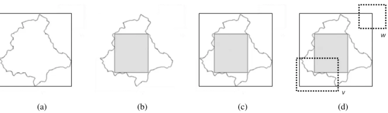
2.3 A region, its approximations and spatial range queries. (a) A region and its
MBR. (b) A region and its MER. (c) A region and its MBR and MER. (d)
Spatial query windowswandv. . . 56
2.4 The multi-step resolution of spatial predicates (adapted from Brinkhoff, Kriegel
& Schneider (1993)). . . 56
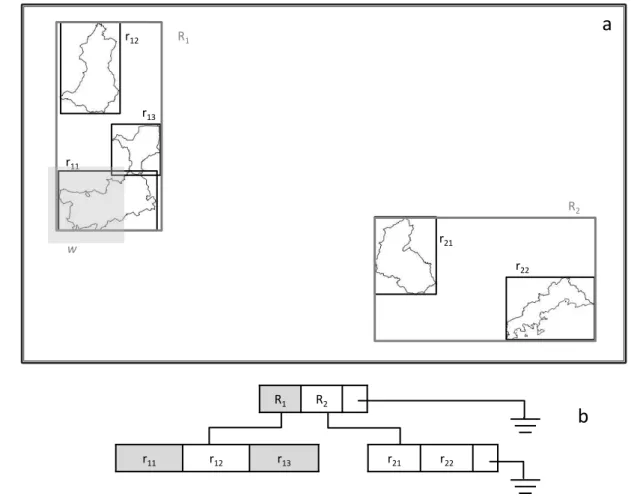
2.5 An R-tree built using cities of customers from the SDW described in Figure
2.1. (a) Cities, their MBRs and the R-tree’s space partitioning method. (b) The
R-tree data structure. . . 58
2.6 Probabilistic modeling of uncertain objects: the location of a vehicle (extracted
from Tao, Xiao & Cheng (2007)). . . 62
2.7 A conceptual model of uncertainty in spatial data (adapted from Fisher (1999)
2.9 Vague regionsAandBand the topological relationships between them
accord-ing to existaccord-ing exact models. . . 73
2.10 Example of vague spatial objects designed according to existing fuzzy models
for spatial vagueness. . . 74
2.11 A simple fuzzy region and its membership function (VERSTRAETE; HALLEZ;
TR ´E, 2006). . . 76
2.12 Evaluating the fuzzy topological relationship between two fuzzy regions. (a)
Pairs of referenceα-cuts in black, and ˜Aα0,B˜α0 in gray. (b) Membership
func-tions and the linguistic labels they assume. . . 78
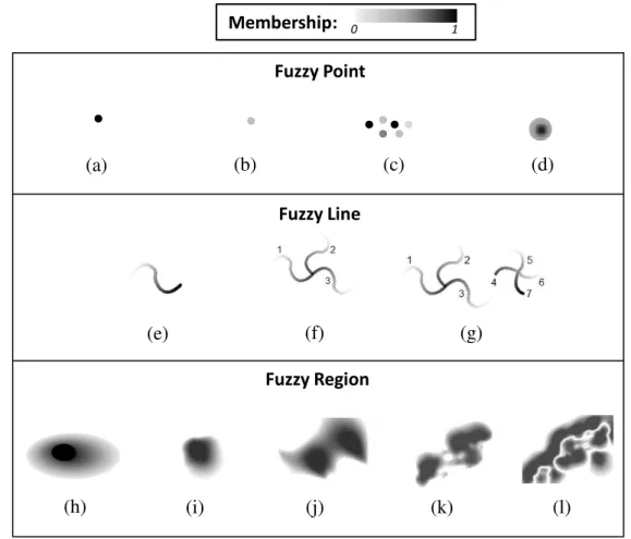
2.13 Examples of implemented fuzzy point, fuzzy lines and fuzzy regions. . . 79
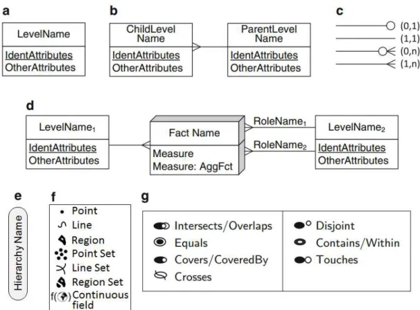
3.1 The graphical notation of the MultiDim conceptual model: (a) Level. (b)
Hier-archy. (c) Cardinalities. (d) Fact with measures and related levels. (e) Hierarchy
name. (f) Spatial data types. (g) Topological relationships. Adapted from
Vais-man & Zim´anyi (2014a). . . 86
3.2 A SDW regarding the maintenance of highways modeled according to the
Mul-tiDim model (extracted from Vaisman & Zim´anyi (2014a)). . . 88
3.3 A SDW regarding the maintenance of highways modeled according to the UML
profile proposed by Boulil, Bimonte & Pinet (2015). . . 90
3.4 The logical design according to the Fuzzy SDW (adapted from Somodevilla &
Petry (2003), Perez, Somodevilla & Pineda (2007)). (a) Sample points and a
studied area. (b) Original schema. (c) The fuzzy MBR. (d) Modified schema. . 93
3.5 A conceptual schema of SDW for CERA (adapted from Jadidi et al. (2013)). . . 94
3.6 Creating fuzzy regions for an arbitrary indicator (adapted from Jadidi et al.
(2014)). (a) A magnified cell and its center. (b) The Gaussian function. (c)
A grid and its vague regions defined over multiple cells. . . 95
3.7 Flow of fertilizer by material by month by spreading region. (a) A spreading
region. (b) The SDW’s fact table. . . 97
3.8 An example of aR-tree. (a) Cities, MBRs and a spatial query window. (b) SDW
(b) SDW data. (c) Bitmap join indices. (d) Data structure of the SB-index. . . . 102
3.10 An example of vague R-tree. (a) Vague regions and their pair of MBRs. (b) Vague R-tree and three point queries. (c) Vague R-tree’s data structure. . . 105
3.11 An example of FMBR R-tree (adapted from Petry, Ladner & Somodevilla (2007)). (a) A fuzzy region and points within it. (b) Data structure. . . 106
4.1 The types of attributes defined in the VSCube Conceptual Model. . . 116
4.2 Instances of crisp spatial attributes: (a) An address. (b) A watershed. . . 117
4.3 The vague spatial attributeν is a composite attribute with a multivalued certi-tude denoted by geometries and a multivalued dubiety denoted by geometries and their membership values. . . 118
4.4 Vague spatial attributes and instances for the pest control case study. (a) An aplied area. (b) A crop. . . 119
4.5 The topological relationships among agricultural lands and crops. . . 121
4.6 The topological relationships among watersheds and agricultural lands. . . 123
4.7 A watershed, an agricultural land and crops. . . 125
4.8 The multidimensional and geographic views provided by the cuboidc0, and the fact f. . . 130
4.9 The matrix of a vague spatial fact. . . 132
4.10 Lattice of cuboids LPesticideApplication, represented according to the bottom-up notation of Ciferri et al. (2013). . . 134
4.11 A subset of the latticeLPesticideApplication. (a) Cuboids. (b) The multidimensional view. (c) The geographic view. (d) Data aggregation. . . 135
4.12 The vague spatial objectzand the spatial query windowq. . . 136
4.13 The results forIRQcertitude elements,IRQdubiety elementsandIRQdubiety elements−mval. (a)IRQcertitude elements. (b)IRQdubiety elements. (c)IRQdubiety elements−mval. . . . 138
4.16 The vague spatial intersection applied to the vague spatial objectsxandy. (a)x
andy. (b)z=V SIntersection(x,y). . . 142
4.17 The vague spatial difference applied to the vague spatial objectsx andy. (a)x andy. (b)z=V SDi f f erence(x,y). . . 143
4.18 A pivoted cuboid. . . 145
4.19 A spatial range query against a TIN. (a) A TIN and a spatial query windoww. (b) Trianglestblackandtgrayof the TIN. . . 149
4.20 Pictograms denoting data types supported by the VSMultiDim conceptual model.152 4.21 Pictograms denoting topological relationships of the VSMultiDim conceptual model. . . 155
4.22 Vague spatial levels: (a) Obtained from a dimension of the pest control case study. (b) Modeled to comply with the HLB case study. . . 156
4.23 A hierarchy of the pest control case study represented according to both the VSCube model and the VSMultiDim model. . . 158
4.24 A hierarchy of the HLB case study represented according to the VSMultiDim model. . . 159
4.25 Hierarchies of the HLB case study represented according to the VSMultiDim model. . . 160
4.26 A conceptual schema of vague SDW for the pest control case study. . . 161
4.27 A conceptual schema of vague SDW for the HLB case study. . . 162
5.1 Separate Tables for Certitude and Dubiety. . . 172
5.2 A vague region and its storage in separate Tables for Certitude and Dubiety. . . 173
5.3 A vague region and its storage in separate Tables for Certitude and Dubiety considering a vague spatial attribute whose both the certitude and the dubiety are monovalued. . . 174
by a single table. . . 175
5.6 A vague region, its MBR and the MBRs of its elements. . . 176
5.7 A single table with a composite primary key. . . 177
5.8 The classesVSElementTypeandVSAttributeTypeand the tableT. . . 178
5.9 A vague region and its representation as an array. . . 178
5.10 The vague spatial attribute represented by a pair of arrays. . . 180
5.11 A vague region and its representation as a pair of arrays. . . 180
5.12 The vague spatial attribute designed as a column for multiple geometries and a column for the array of membership values. . . 182
5.13 A vague region stored as a multiple geometry and an array of membership values.183 5.14 The logical design for the vague spatial attribute with monovalued certitude and monovalued dubiety. . . 185
5.15 The storage of a vague region whose both certitude and dubiety are monovalued. 185 5.16 Shortcomings of both the 2D geometry type with measure and the 3D geometry type: (a) A vague point set. (b) A vague line. (c) Two elements of a vague region. . . 186
5.17 Examples of the application of Rule 2VS to obtain the vague spatial level tables CropandInfection. . . 192
5.18 Mapping rules applied to a pair of related vague spatial levels. . . 195
5.19 The logical schema of the vague SDW regarding the HLB disease. . . 197
5.20 A vague spatial fact table. (a) The schema. (b) A vague spatial fact set. . . 201
5.21 A vague spatial fact table with a vague spatial measure for areas where pesti-cides were applied to. . . 203
5.22 Intersections among elements of A1 and C1. (a) A1 and C1. (b) Intersection among elements ofA1 andC13. (c) Merging the geometries from (b). (d) Inter-section among elements ofA1andC11. (e) Merging the geometries from (d). . 204
6.2 Creating vague point sets: (a) Processing the real polygon. (b) The vague point
set. . . 239
6.3 The spatial query windowwcontaining two vague point sets. . . 240
6.4 Performance results of the DBMS for the vague SDW containing vague point
sets: (a) Storage requirements. (b) Query processing. . . 241
6.5 The schema of the vague SDW storing vague regions: (a) Incomplete schema.
(b) Tables to complete the schema. . . 242
6.6 From real polygons to vague regions: (a) Processing the real polygon. (b) The
obtained vague region. . . 243
6.7 The spatial query windowwintersecting several vague regions of the vague SDW.245
6.8 Results for the DBMS and indices for SDWs: (a) Average elapsed time. (b)
Fraction of the vague spatial predicate. . . 246
6.9 The vague SDW storing vague regions in a separate table. . . 248
6.10 Elapsed time to process VSRQobject over the vague SDW containing vague
regions. . . 250
6.11 A vague region and its approximations: (a) The MIP5 on the certitude. (b) The
MBR on the vague region and the MIP5 on the certitude. . . 252
6.12 A vague region in tones of gray, its approximations with black continuous
contour and spatial range queries with dashed rectangles: (a) A CRQob ject
againstOMBR. (b) ACRQcertitude againstOMBRCMBR. (c) AnIRQob ject against
OMBRCMIP5. (d) Another IRQob ject against OMBRCMIP5. (e) An IRQcertitude
againstOMBROMIP5CMBRCMIP5. . . 259
6.13 A vague region, its elements and vague spatial predicates regarding the dubiety:
(a) ACRQdubiety. (b) AnIRQdubiety. (c) A query window into the holes. . . 262
6.14 Vague spatial range queries. (a) Against MBRs. (b) Against MBRs and MIP5s. 268
6.15 The schema of both the synthetic vague SDW and the real vague SDW. . . 273
6.16 Two vague regions and one spatial query windoww. . . 273
6.17 Results for IRQobject and IRQdubiety issued over the real vague SDW: (a)
time. (b) Average number of candidates. . . 279
6.19 The performance to process IRQobject and IRQdubiety over the synthetic vague
SDW. . . 281
6.20 The performance to process the IRQcertitude over the synthetic vague SDW. . . 283
6.21 Average elapsed time to process CRQobject and CRQdubity over the synthetic
vague SDW. . . 284
6.22 Average elapsed time to process CRQcertitude over the synthetic vague SDW. . 286
6.23 Average elapsed time to process VSRQobject over the synthetic vague SDW. . 288
6.24 Time spent to build different configurations of the VSB-index. . . 290
1.1 Examples of queries for the analysis of the pest control activities. . . 34
1.2 Examples of queries for the analysis of of HLB control. . . 37
2.1 Multidimensional queries extended with spatial predicates. . . 47
2.2 Nomenclatures adopted by exact models for components of a vague spatial object. 68
2.3 Comparing exact models, fuzzy models and implementations for fuzzy models. 83
3.1 Comparing existing work on SDW design to conceptual modeling and logical
design of vague SDWs introduced in this thesis. . . 108
3.2 Comparing existing work on design of SDWs characterized by spatial
vague-ness to the design of vague SDWs described in this thesis. . . 109
3.3 Comparing indices for SDW and indices for vague regions to the VSB-index. . 110
4.1 Types that the attributesxiandxi+1can assume. . . 122
4.2 Categories of hierarchies of the VSCube conceptual model. . . 126
5.1 The approaches described in Sections 5.2.1 to 5.2.6 and the goals they achieve. 187
5.2 Operations on vague spatial attributes. . . 219
5.3 Accessors: methods’ signatures and descriptions. . . 220
5.4 Vague spatial predicates: methods’ signatures and descriptions. . . 223
5.5 Vague spatial aggregation functions: methods’ signatures and descriptions. . . . 228
5.6 Classes of slice and dice operations. . . 230
5.7 Classes of roll-up and drill-down operations. . . 230
5.8 The logical design of vague SDWs and the corresponding guidelines or
6.2 Spatial range queries of the workload. . . 275
6.3 Summary of the results obtained with the experimental evaluation of the
CHAPTER 1 – INTRODUCTION 29
1.1 The Pest Control Case Study . . . 32
1.2 The HLB Case Study . . . 34
1.3 Thesis Organization . . . 37
CHAPTER 2 – THEORETICAL FOUNDATIONS 41
2.1 Spatial Data Warehouse Design . . . 41
2.1.1 Conceptual Modeling . . . 41
2.1.1.1 Entity-Relationship Model and Unified Modeling Language . 42
2.1.1.2 Multidimensional Modeling . . . 43
2.1.1.3 Spatial Data . . . 44
2.1.1.4 Multidimensional and Spatial Data Cubes . . . 45
2.1.2 Logical Design . . . 46
2.1.2.1 Relational Databases . . . 47
2.1.2.2 Spatial Extensions of Database Management Systems . . . . 48
2.1.2.3 Relational Representation of Spatial Data Warehouses . . . . 49
2.1.3 Physical Design . . . 52
2.1.3.1 Bitmap Index and Bitmap Join Index . . . 52
2.1.3.2 Spatial Indices . . . 54
2.2.1.1 Probabilistic Data Warehouses . . . 61
2.2.1.2 Probabilistic Spatial Data . . . 61
2.2.2 Fuzzy Data . . . 63
2.2.2.1 Fuzzy Data Warehouses . . . 63
2.3 Spatial Vagueness . . . 65
2.3.1 Exact Models for Spatial Vagueness . . . 67
2.3.1.1 Vague Spatial Data Types . . . 68
2.3.1.2 Vague Spatial Geometric Set Operators . . . 70
2.3.1.3 Vague Topological Relationships . . . 71
2.3.2 Fuzzy Models for Spatial Vagueness . . . 72
2.3.2.1 Fuzzy Spatial Data Types . . . 72
2.3.2.2 Fuzzy Spatial Operators . . . 76
2.3.2.3 Fuzzy Spatial Topological Relationships . . . 77
2.3.3 Implementations for Fuzzy Models . . . 78
2.3.3.1 Spatial Plateau Objects . . . 79
2.3.3.2 Lines with Gradual Transitions . . . 80
2.3.3.3 Bitmaps . . . 80
2.3.3.4 Triangulated Irregular Networks . . . 81
2.3.3.5 Fuzzy Minimum Bounding Rectangles . . . 81
2.3.4 Summary . . . 82
CHAPTER 3 – RELATED WORK 85
3.1 Conceptual Modeling and Logical Design of Spatial Data Warehouses . . . 85
3.1.1 The MultiDim Conceptual Model . . . 86
3.1.2 UML Profiles . . . 88
3.2 Spatial Vagueness in Spatial Data Warehouses . . . 92
3.2.1 The Fuzzy Spatial Data Warehouse . . . 92
3.2.2 Conceptual Frameworks for Risk Assessment . . . 94
3.2.3 The RADSOLAP Method . . . 96
3.2.4 Discussion . . . 98
3.3 Indices for Spatial Data Warehouses . . . 99
3.3.1 aR-tree . . . 99
3.3.2 SB-index . . . 101
3.3.3 Discussion . . . 103
3.4 Indices for Vague Regions . . . 104
3.4.1 Vague R-tree . . . 104
3.4.2 FMBR R-tree . . . 105
3.4.3 Discussion . . . 107
3.5 Summary . . . 107
CHAPTER 4 – CONCEPTUAL DESIGN OF VAGUE SPATIAL DATA WAREHOUSES111
4.1 Conceptual Modeling of Vague Spatial Data Warehouses . . . 112
4.2 Attributes . . . 115
4.3 Hierarchies . . . 120
4.3.1 Hierarchy Operator . . . 120
4.3.2 Properties of Hierarchies . . . 123
4.3.3 Categories of Hierarchies . . . 126
4.4 Multidimensional Cube with Vague Spatial Data . . . 127
4.4.1 Dimensions . . . 127
4.4.2 Measures . . . 128
4.4.5 Lattice of Cuboids . . . 132
4.5 Vague Spatial Predicates . . . 134
4.5.1 Spatial Range Queries . . . 135
4.5.2 The Vague Spatial Range Query . . . 138
4.6 Vague Spatial Aggregation Functions . . . 140
4.6.1 Vague Spatial Union . . . 140
4.6.2 Vague Spatial Intersection . . . 141
4.6.3 Vague Spatial Difference . . . 142
4.7 Vague Spatial Online Analytical Processing . . . 144
4.8 Reusing Existing Models and Implementations . . . 146
4.8.1 Arbitrary Geometries . . . 146
4.8.2 Bitmaps . . . 147
4.8.3 Triangulations . . . 147
4.8.4 Lines with Gradual Transitions . . . 150
4.9 The Vague Spatial MultiDim Conceptual Model . . . 151
4.9.1 Fundamentals . . . 152
4.9.1.1 Data Types . . . 152
4.9.1.2 Certitude and Dubiety . . . 154
4.9.1.3 Vague Topological Constraints . . . 154
4.9.2 Attributes, Levels and Members . . . 155
4.9.3 Dimensions and Hierarchies . . . 157
4.9.4 Fact and Measures . . . 160
4.10 Summary . . . 164
CHAPTER 5 – LOGICAL DESIGN OF VAGUE SPATIAL DATA WAREHOUSES 167
5.2.1 Separate Tables for Certitude and Dubiety . . . 171
5.2.2 A Single Table for Certitude and Dubiety . . . 174
5.2.3 User Defined Types . . . 177
5.2.4 A Pair of Arrays . . . 179
5.2.5 One Multiple Geometry And One Array of Membership Values . . . . 181
5.2.6 Monovalued Certitude and Monovalued Dubiety . . . 184
5.2.7 2D Geometry With Measure or 3D Geometry . . . 184
5.2.8 Discussion . . . 186
5.3 Vague Spatial Attribute . . . 187
5.4 Vague Spatial Level and Vague Spatial Member . . . 191
5.5 Hierarchies . . . 194
5.6 Fact and Vague Spatial Measure . . . 195
5.7 Vague Spatial Fact . . . 197
5.7.1 Relational Representation . . . 198
5.7.2 Numeric Measures and Crisp Spatial Measures . . . 199
5.7.3 Vague Spatial Measures . . . 201
5.7.4 Loading a Vague Spatial Fact Table . . . 205
5.7.5 Discussion . . . 206
5.8 Vague Topological Constraints . . . 208
5.8.1 Pairwise Evaluation of Sets of Topological Relationships . . . 208
5.8.2 Hierarchy . . . 211
5.8.3 Spatial Fact . . . 214
5.8.4 Intra Level and Intra Fact . . . 217
5.9 Vague Spatial Online Analytical Processing . . . 219
5.9.3 Vague Spatial Aggregation Functions . . . 228
5.9.4 Slice-and-Dice, Roll-Up, and Drill-Down . . . 229
5.10 Summary . . . 231
CHAPTER 6 – PHYSICAL DESIGN OF VAGUE SPATIAL DATA WAREHOUSES 235
6.1 Indexing Vague Spatial Data Warehouses . . . 235
6.2 Evaluation of a DBMS and of Indices for Spatial Data Warehouses . . . 237
6.2.1 Containment Range Queries against Vague Point Sets . . . 237
6.2.1.1 Workbench and Platforms . . . 238
6.2.1.2 Workload . . . 240
6.2.1.3 Results . . . 240
6.2.2 Intersection Range Queries against Vague Regions . . . 241
6.2.2.1 Workbench and Platforms . . . 242
6.2.2.2 Workload . . . 243
6.2.2.3 Results . . . 245
6.2.3 Vague Spatial Range Queries against Vague Regions . . . 246
6.2.3.1 Workbench and Platforms . . . 247
6.2.3.2 Workload . . . 247
6.2.3.3 Extending the SB-index . . . 249
6.2.3.4 Results . . . 249
6.2.4 Discussion . . . 250
6.3 The Vague Spatial Bitmap Index . . . 251
6.3.1 Maximum Area Inscribed Polygon . . . 252
6.3.2 Data Structure . . . 252
6.3.3 Building Operation . . . 253
6.3.4.2 Filtering with a Conservative Approximation and a
Progres-sive Approximation . . . 259
6.3.4.3 Particularities of Querying the Dubiety . . . 261
6.3.4.4 Calling the Procedures . . . 262
6.3.5 Processing Queries Containing a Vague Spatial Range Query . . . 264
6.3.5.1 Filtering with a Conservative Approximation . . . 266
6.3.5.2 Filtering with a Conservative Approximation and a
Progres-sive Approximation . . . 268
6.3.5.3 Calling the Procedures . . . 270
6.4 Evaluation of the VSB-index . . . 271
6.4.1 Experimental Setup . . . 272
6.4.1.1 Workbench and Platforms . . . 272
6.4.1.2 Workload . . . 275
6.4.2 Intersection Range Queries over the Real Vague SDW . . . 276
6.4.2.1 IRQobject and IRQdubiety . . . 277
6.4.2.2 IRQcertitude . . . 278
6.4.3 Intersection Range Queries over the Synthetic Vague SDW . . . 280
6.4.3.1 IRQobject and IRQdubiety . . . 280
6.4.3.2 IRQcertitude . . . 282
6.4.4 Containment Range Queries over the Synthetic Vague SDW . . . 282
6.4.4.1 CRQobject and CRQdubiety . . . 283
6.4.4.2 CRQcertitude . . . 285
6.4.5 Vague Spatial Range Queries over the Synthetic Vague SDW . . . 285
6.4.5.1 Test Configurations . . . 286
6.4.5.2 Results . . . 287
CHAPTER 7 – CONCLUSION AND FUTURE WORK 295
REFERENCES 301
GLOSSARY 317
APPENDIX A – USER-DEFINED FUNCTIONS 319
Chapter 1
I
NTRODUCTION
Decision-making support has gained the attention of researchers of data warehouse (DW),
online analytical processing (OLAP), and geographic information system (GIS). Spatial data
warehouse (SDW) and spatial online analytical processing (SOLAP) are remarkable
achieve-ments that resulted from their research. A SDW is a subject-oriented, integrated, time-variant,
voluminous, non-volatile and multidimensional database that stores spatial data and
conven-tional data (numeric and alphanumeric) (STEFANOVIC; HAN; KOPERSKI, 2000; FIDALGO et al.,
2004;SILVA et al., 2010; VAISMAN; ZIM ´ANYI, 2014b). Fact, dimension, and hierarchy are core
concepts of a SDW. A fact denotes the scores of business activities through numeric measures or
spatial measures, while dimensions hold conventional attributes and spatial attributes that
con-textualize the values of the measures. Hierarchies associate dimension’s attributes of coarser
and finer granularity. When these attributes are spatial, the association is described by a
topo-logical relationship (e.g. within).
SOLAP aids the decision-making process by providing spatial analysis combined with
multidimensional analytical queries that run over the SDW (B ´EDARD; MERRETT; HAN, 2001;
BIMONTE; TCHOUNIKINE; MIQUEL, 2005). SOLAP operations process both conventional and
spatial data. For instance, a roll-up operation aggregates not only numeric data with functions
such as sum, but also aggregates spatial data using the geometric union (STEFANOVIC; HAN;
KOPERSKI, 2000;SILVA et al., 2008;GOMEZ et al., 2009;BOULIL; BIMONTE; PINET, 2015). In
ad-dition, spatial range queries select spatial data that satisfy a given topological relationship (e.g.
intersects and within) with respect to an ad hoc spatial query window (PAPADIAS et al., 2001;
SIQUEIRA et al., 2010).
In SDWs, spatial data are modeled either as spatial objects or as continuous fields (
STE-FANOVIC; HAN; KOPERSKI, 2000;VAISMAN; ZIM ´ANYI, 2009;BIMONTE; KANG, 2010;GASCUE ˜NA;
ob-jects are crisp in the sense that they assume definite extent, boundary, and shape, e.g. the
territory of a city. They are commonly implemented using vector geometries provided by the
underlying DBMS (HOEL, 2008). Continuous fields represent phenomena that change
contin-uously in space, e.g. elevation (C ˆAMARA; FREITAS; CASANOVA, 1995; C ˆAMARA et al., 2014).
They are often implemented as raster and triangulated irregular networks (HOEL, 2008).
However, spatial data are susceptible to imperfections. Spatial vagueness is one kind of
spatial data imperfection concerning the difficulty of distinguishing an object shape from its
neighborhood, since the concepts used to describe the spatial information are not defined
pre-cisely (WORBOYS, 1998; BEJAOUI, 2009). As a result, it is not possible to be sure if the parts
of a spatial object belong completely to it, or possibly belong to it, or simply do not belong to
it (PAULY; SCHNEIDER, 2010). A vague spatial object has an extent, but it inherently cannot or
does not have a precisely definable boundary and/or interior. Consequently, it is not rigorously
bounded by a sharp line and might have a blurred interior (BURROUGH, 1996; SCHNEIDER,
2014). Spatial vagueness has been considered in applications for agriculture (BEJAOUI et al.,
2009;EDOH-ALOVE et al., 2014), coastal erosion (DILO, 2006; JADIDI et al., 2014), volcanic
cri-sis management (PEREZ; SOMODEVILLA; PINEDA, 2010), among others (BURROUGH; FRANK,
1996).
Spatial vagueness has been addressed by distinct models that assign membership degrees to
vague concepts: exact models (COHN; GOTTS, 1996;CLEMENTINI; FELICE, 1996;BEJAOUI et al.,
2009, 2010;PAULY; SCHNEIDER, 2010) and fuzzy models (DILO; BY; STEIN, 2007;SCHNEIDER,
2008; TANG; KAINZ; WANG, 2010; HAZARIKA; HAZARIKA, 2012; SCHNEIDER, 2014). Exact
models are mostly based on crisp spatial data types, while fuzzy models adopt the fuzzy set
theory as their mathematical fundamentals. There is not a commonly accepted terminology
to define concepts related to imperfections of spatial data (DEVILLERS et al., 2010). In this
thesis, the terms vague and fuzzy differ exclusively in the approach used to define the model.
Therefore, vague spatial data can be modeled either according to a vague spatial data type from
an exact model or to a fuzzy spatial data type from a fuzzy model.
Existing models for representing spatial vagueness do not provide multidimensional
analy-sis combined with spatial analyanaly-sis. However, such combination is essential for a SOLAP tool to
query a SDW. Spatial vagueness was tackled exclusively in data cleansing and integration tasks,
before the design of the SDW schema, for natural phenomena whose indeterminate boundaries
need to be re-measured at different epochs (B ´EDARD; MERRETT; HAN, 2001). Since the design
of SDWs typically considers crisp spatial objects, it prevents some types of decision-support
gained the attention of researchers and recent work in the literature consider spatial vagueness
in the design of SDWs (PEREZ; SOMODEVILLA; PINEDA, 2010;JADIDI et al., 2013;EDOH-ALOVE;
BIMONTE; B ´EDARD, 2014; EDOH-ALOVE et al., 2014). Those work rely upon the advances on
multidimensional modeling (VAISMAN; ZIM ´ANYI, 2014b;BOULIL; BIMONTE; PINET, 2015),
sys-tems of both vague and fuzzy spatial data types (BURROUGH; FRANK, 1996; DILO; BY; STEIN,
2007; PAULY; SCHNEIDER, 2010), and implementations for these systems (VERSTRAETE et al.,
2005;SCHNEIDER, 2014).
Nevertheless, existing work focus exclusively on conceptual design of SDWs (JADIDI et al.,
2013), or on logical design of SDWs (PEREZ; SOMODEVILLA; PINEDA, 2010), or do not
con-sider different models to represent spatial vagueness in the design of SDWs (EDOH-ALOVE;
BIMONTE; B ´EDARD, 2014; EDOH-ALOVE et al., 2014). Furthermore, the physical design of a
SDW does not comprise an index to improve the performance of multidimensional queries
ex-tended with spatial predicates involving vague spatial data. Rather, existing indices process
either multidimensional queries (WU et al., 2009; LANE; POTINENI, 2014), or spatial predicates
involving crisp spatial data (GUTTMAN, 1984;AOKI, 1998;ORACLE. . ., 2014;OBE; HSU, 2015),
or spatial predicates involving vague spatial data (PETRY; LADNER; SOMODEVILLA, 2007), or
multidimensional queries extended with spatial predicates involving crisp spatial data (
PAPA-DIAS et al., 2001;SIQUEIRA et al., 2012b).
On the other hand, in this thesis, spatial vagueness is considered to design and query the
SDW. Consequently, the vague spatial data warehouse (vague SDW) and the vague spatial
on-line analytical processing (vague SOLAP) are obtained. The results of the investigations on
conceptual modeling, logical design, and physical design of the vague SDW have provided the
following contributions:
• the Vague Spatial Cube (VSCube) conceptual model that enables the creation of concep-tual schemata for vague SDWs using data cubes and provides vague spatial aggregation
functions and vague spatial predicates to query vague spatial data from measures and
dimensions;
• the Vague Spatial MultiDim (VSMultiDim) conceptual model that provides visual rep-resentations for the concepts and enables the creation of conceptual schemata for vague
SDWs using diagrams;
• guidelines for designing relational schemata and integrity constraints for vague SDWs, and for extending the SQL language to enable vague SOLAP;
queries against vague SDWs.
In order to illustrate the applicability of the vague SDW and the aforementioned
contri-butions, two case studies concerning agriculture are described and used throughout this thesis
to exemplify concepts. The pest control case study described in Section 1.1 addresses a real
problem whose existing solutions mostly neglect spatial vagueness. The huanglongbing (HLB)
case study detailed in Section 1.2 tackles a real problem in citriculture that has been
investi-gated by the Brazilian Agricultural Research Corporation (Embrapa), but that had not yet been
addressed using a vague SDW. Section 1.3 outlines the chapters of this thesis and summarizes
the aforementioned contributions.
1.1
The Pest Control Case Study
Precision agriculture has been adopted in the management of farms to optimize returns on
inputs while preserving resources. Spatial and temporal characteristics of crops are processed
in decision support systems (INAMASU et al., 2011). For instance, remote sensing images are
provided as input to classification algorithms, e.g. k-means, for identification of crops and
their characteristics (RECIO et al., 2013). The goal is to map the crop in order to apply a suitable
pesticide rate. The output of the classification comprises some crops as crisp regions and several
crops as vague regions.
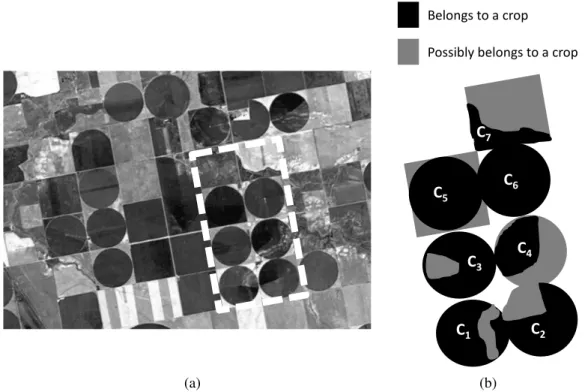
Figure 1.1a shows a remote sensed image and crops highlighted inside a white dashed
rectangle. One crop is identified as being crisp and is shown in Figure 1.1b: C6. On the other
hand, the remaining crops intrinsically have a vague shape, e.g. the cropC1 has two parts that
belong to it in black and one part that may belong to it in gray, and the cropC5has one part that
belongs to it in black and four parts that may belong to it in gray.
The combination of remotely sensed imagery and variable rate technology enables the
ap-plication of pesticides at specific locations (RECIO et al., 2013). Pesticides such as herbicides,
insecticides, fungicides and defoliants are applied aerially to crops, with some fraction
inter-cepted by foliage and some fraction reaching the soil. Methods of application vary from ground
equipment to aircraft, and the material can be applied as solids, dispersions, emulsions or
so-lutions (LEONARD; KNISEL; STILL, 1987). Pesticides are not applied uniformly over the extent,
due to variable spraying according to the weed area, real-time sensory and fuzzy control used to
regulate dose of drugs (SHI et al., 2008). In addition, dissipation, plant transpiration and runoff
influence the distribution of pesticide in a given extent (NEITSCH; ARNOLD; WILLIANS, 2011).
Fig-(a)
C5
C6 C7
C3 C4
C1 C2
Belongs to a crop
Possibly belongs to a crop
(b)
Figure 1.1: Crops in remote sensed image and after identification. (a) A remote sensed image (adapted from Crop Circles in Kansas, by NASA Image of the Day Gallery). (b) Identified crops.
ure 1.2a, indicate that the possibility of application is higher in the darker gradient than in the
brighter gradient.
A1
C1
(a)
C11
0.25 tons
C12
(b) (c)
A1 100%
80%
50%
30%
(d)
Figure 1.2: An applied area of pesticideA1over the cropC1. (a)A1overC1. (b)A1overC11. (c)A1
overC13. (d) Subsets ofA1.
In addition to estimate where pesticides were applied, another relevant measure in the study
is the amount in tons of pesticides applied. For instance, considering that 0.3 t were applied over
A1, some portions of pesticides were applied over parts of crops, as follows: 0.25 t were applied
over the partC11that certainly belongs toC11, as shown in Figure 1.2b; no pesticide was applied
over the partC12that certainly belongs toC1; and 0.05 t were applied over the partC13that may
represen-Table 1.1: Examples of queries for the analysis of the pest control activities.
Query Description
PC1 Retrieve the amount of pesticides applied and areas where pesticides were applied to by pesticide by date by crop.
PC2 Retrieve the amount of pesticides applied and areas where pesticides were applied to by pesticide by date by parts that certainly (or possibly) belong to a crop.
PC3 Retrieve the amount of pesticides applied and areas where pesticides were applied to by pesticide type by month by agricultural land.
PC4 Retrieve the amount of pesticides applied and areas where pesticides were applied to by pesticide type by month by agricultural land, for herbicides applied in 2012 whose applied areas certainly intersect a spatial query window provided by the user.
tation of a continuous applied area is obtained as subsets having a possibility of application,
according to Figure 1.2d, forA1and possibilities of 100%, 80%, 50% and 30%. Such
represen-tation use geometric shapes and the corresponding possibility (membership) values. Dates of
pesticide applications are also recorded.
Agricultural lands from different owners are identified through the same procedure and
have broad boundaries. Each agricultural land maintains several crops, but one crop is
asso-ciated to at most one agricultural land. Aiming at correlating water quality and pesticide use,
watersheds were included in the application and gathered from the database of the hydrological
local department. Each watershed contains several agricultural lands.
Crops, areas of pesticide application, and agricultural lands are affected by spatial
vague-ness, while watersheds are crisp regions. The areas where pesticides were applied to and the
amounts of applied pesticides in tons are reported by pesticide by crop by date to benefit the
analysis of the agricultural and the environmental impacts. Table 1.1 lists a few queries used
for the analysis of the pest control activities.
1.2
The HLB Case Study
Huanglongbing(HLB), also known as greening, is the world’s most serious citrus disease
(BOV ´E, 2014). A bacteria-carrying psyllid injects the bacterium into a healthy tree while feeding
from it. Visual inspections of all trees of the plot are carried out monthly throughout multiple
years to detect symptomatic and infected trees. The symptom severity is a value estimated after
often high symptom severity, some infected trees show no symptoms during a period.
Studying the spatial distribution of infection is valuable to motivate control practices, e.g.
eradication of symptomatic trees and replacement by healthy trees. HLB spread is analyzed
(GOTTWALD, 2010): (i) by tree, by plot, by farm, by city; and (ii) by group of certainly and
possibly infected trees, by region with several groups. Given a certainly infected tree, adjacent
trees within row and across row are possibly infected. The possibility of infection is higher
as closer a tree is from an infected tree. A group may encompass up to 572 trees and the
distance between groups was once estimated to be within 25 to 30 meters (GOTTWALD; GRAC¸ A;
BASSANEZI, 2007). The edge effect determines that infected regions often overlap more than
one plot, mainly when neighbor farms do not comply with a regional policy of HLB control.
Furthermore, a recent study reported decreasing psyllid abundance with increased elevation,
e.g. no psyllids were collected at an elevation above 600 meters (JENKINS; HALL; GOENAGA,
2015).
The Brazilian Agricultural Research Corporation (Embrapa) studies HLB. For instance,
Jorge & Inamasu (2014) described an application whose main features are the following. Farms,
their plots, and plot’s trees are mapped. All of them have exact location and boundaries. A farm
has an owner and comprises several plots. In a plot, trees of a given plant are grown. Monthly,
inspectors examine all trees and annotate a status, i.e. “healthy”, “infected”, or “eradicated”.
The dataset used by Jorge & Inamasu (2014) has been kindly provided for use in this thesis.
In order to comply with the characteristics of HLB infection, the following features extend the
cited application.
The HLB infection is mapped monthly. An inspector examines a tree and estimates a
pos-sibility of infection in [0,1] to the tree’s location. The pospos-sibility of infection indicates whether
the tree’s location belongs to the HLB infection and quantifies the membership degree. For each
location where the possibility of infection is 1, locations of adjacent trees within row and across
row are assigned a possibility of infection in ]0,1[ according to a distance function. An infected
group is composed of adjacent locations that had a possibility of infection assigned.
After the complete examination of the farm, the extent occupied by the HLB infection is
outlined as a region that covers one or more infected groups. Clustering techniques can be
applied to outline infected regions, e.g. α-hull (EDELSBRUNNER; KIRKPATRICK; SEIDEL, 1983)
and fuzzy c-means (BEZDEK; EHRLICH; FULL, 1984). An infected region is composed both by
parts where the possibility of infection is 1 and by parts where the possibility of infection is in
]0,1[. It may overlap more than one plot.
Figure 1.3b zooms into the rectangular area highlighted in Figure 1.3a and shows two certainly
infected trees recognized in a given month: the red and the orange, each one in a plot. These
trees belong to the red group and to the orange group as shown in Figure 1.3c. Each tree in a
group has a possibility of infection. Both the orange group and the red group belong to the same
infected region shown in Figure 1.3d, which overlaps bothPlot1andPlot2, even though a road separates these plots. Figure 1.3e shows a discrete representation of the continuous infected
region exemplified in Figure 1.3d, according to the possibility of infection.
(a) (b) (c)
(d) (e)
Figure 1.3: HLB infection. (a) Plots. (b) Two infected trees. (c) Two infected groups. (d) Two groups and a continuous representation for an infected region. (e) Two groups and a discrete representation for an infected region.
In addition to examine a tree and estimate a possibility of infection, the inspector also
as-signs the HLB symptom severity as a value within 0 and 9. Furthermore, the inspector indicates
whether the examined tree must be eradicated or not. If a tree is eradicated, then its eradication
date is assigned. Therefore, each tree must also have a date when it was planted, while the date
of eradication due to HLB infection is initially unknown. Table 1.2 lists a few queries used for
Table 1.2: Examples of queries for the analysis of of HLB control.
Query Description
HLB1 Retrieve an infection’s location and possibility and the symptom severity by tree by infected group by month by inspector.
HLB2 Retrieve infections’ location and maximum possibility by plot by quarter of 2014.
HLB3 Retrieve the average symptom severity by infected group by month in 2014.
HLB4 Retrieve the number of eradicated trees by plot by year by team.
HLB5 Retrieve the number of eradicated trees by year by team, such that infected regions intersect a spatial query window provided by the user.
HLB6 Retrieve the number of certainly infected trees located between 500m and 600m by plot by month in a given city between January and June, 2014.
HLB7 Retrieve infected regions identified in a given city between January and March, 2014, such that infection possibility was greater than 80%.
1.3
Thesis Organization
Chapter 2 addresses the main concepts that are necessary to comprehend this thesis,
con-cerning SDW and spatial vagueness. Firstly, fundamentals of conceptual modeling, logical
design and physical design for SDWs are surveyed. Secondly, spatial vagueness is
character-ized and the fundamentals of the main approaches for spatial vagueness are summarcharacter-ized. Exact
models, fuzzy models and implementations for fuzzy models are revised according to their data
types, operators, and topological relationships.
Chapter 3 surveys and discusses existing work in the literature that are related to this thesis.
The main characteristics of existing conceptual models for SDW are reported in order to
iden-tify requirements of a conceptual model for vague SDWs. Similarly, existing work aimed at the
logical design of SDWs are addressed to determine a baseline for the logical design of vague
SDWs. Furthermore, indices for SDWs have their data structures and query processing
algo-rithms studied to verify the adequacy for indexing vague spatial data. Finally, existing indices
for vague regions are also surveyed regarding the data types they support, the query processing
algorithms they offer, and the spatial predicates they resolve.
Chapter 4 addresses conceptual design of vague SDWs and describes two major
contri-butions of this thesis: the VSCube conceptual model and the VSMultiDim conceptual model.
spatial objects as geometric shapes and their corresponding membership values, both in
dimen-sions or as measures in a fact. Furthermore, values of measures are allowed to be assigned to
parts of a vague spatial object. Vague spatial aggregation functions (e.g. vague spatial union),
vague spatial predicates (e.g. vague spatial range queries) and vague SOLAP operations (e.g.
drill-down and roll-up) are described to enable spatial analysis combined with multidimensional
exploitation of the data cube. The VSMultiDim conceptual model extends an existing
concep-tual model for SDWs by enabling vague spatial attributes in dimensions or as measures in a
fact, and by specifying constraints involving vague spatial data. Differently from the VSCube
model, the VSMultiDim model provides a graphical notation to allow the creation of diagrams
that represent the multidimensional conceptual schema of the vague SDW. Both the VSCube
and the VSMultiDim models overcome related work in expressiveness, as those models tackle
both vague spatial data types and fuzzy spatial data types.
Chapter 5 focuses the logical design of vague SDWs underlying relational database
manage-ment systems (DBMSs) with an extension for spatial data. Alternative logical designs for vague
spatial attributes are duly described and compared. Mapping rules are provided to transform the
conceptual schema of a vague SDW into a logical schema. These mapping rules address
at-tributes, dimensions, hierarchies, measures, and fact. In addition, an specific design for the fact
allows values of measures to be assigned to parts of a vague spatial object. Vague SOLAP is
enabled by extending SQL and implementing operations for accessing vague spatial data,
pro-cessing vague spatial predicates and computing aggregation of vague spatial data. Constraints
are specified and implemented to maintain the integrity of the vague SDW. The guidelines for
designing schemata and constraints for SDWs are also part of the major contributions of this
thesis.
Chapter 6 focuses the physical design of vague SDWs and describes one of the major
con-tributions of this thesis: the VSB-index. Firstly, an experimental evaluation of a database
man-agement system and of existing indices for SDWs identify bottlenecks and their limitations to
provide a reasonable performance to process queries over vague SDWs. Secondly, the
VSB-index is introduced and described. Thirdly, an experimental evaluation of the VSB-VSB-index is
described and the benefits for the performance to process queries over vague SDWs are
dis-cussed.
The development of this doctoral research project resulted in the following publications that
are related to this thesis:
1. Siqueira, Thiago Lu´ıs Lopes; Ciferri, Cristina Dutra de Aguiar; Times, Val´eria Ces´ario;
conceptual model. Geoinformatica (Dordrecht. Online), v. 18, p. 313-356, 2014.
2. Siqueira, Thiago Lu´ıs Lopes; Ciferri, Ricardo Rodrigues; Zim´anyi, Esteban. Extending
the MultiDim conceptual model to enable the design of vague spatial data warehouses.
In: Dutch Belgian Database Day, 2014, Anvers, Belgium. Online abstract available at:
http://adrem.ua.ac.be/sites/adrem.ua.ac.be/files/abstract 14.pdf.
3. Siqueira, Thiago Lu´ıs Lopes; Ciferri, Cristina Dutra de Aguiar; Times, Val´eria Ces´ario;
Ciferri, Ricardo Rodrigues. Towards Vague Geographic Data Warehouses. In:
Inter-national Conference on Geographic Information Science, 2012, Columbus, OH, USA.
Lecture Notes in Computer Science. New York: Springer-Verlag, 2012. v. 7478. p.
173-186.
4. Siqueira, Thiago Lu´ıs Lopes; Mateus, Rodrigo Costa; Ciferri, Ricardo Rodrigues; Times,
Val´eria Ces´ario; Ciferri, Cristina Dutra de Aguiar. Querying Vague Spatial Information
in Geographic Data Warehouses. In: The 14th AGILE International Conference on
Geo-graphic Information Science, 2011, Utrecht, Netherlands. Lecture Notes in
Geoinforma-tion and Cartography: Advancing GeoinformaGeoinforma-tion Science for a Changing World, 2011.
v. 1. p. 379-397.
5. Siqueira, Thiago Lu´ıs Lopes; Oliveira, Jo˜ao Celso Santos; Times, Val´eria Ces´ario; Ciferri,
Cristina Dutra de Aguiar; Ciferri, Ricardo Rodrigues. Indexing Vague Regions in Spatial
Data Warehouses. In: XIV Brazilian Symposium on Geoinformatics, 2013, Campos do
Jord˜ao, SP, Brazil. XIV Brazilian Symposium on Geoinformatics, Proceedings, 2013. p.
158-169.
6. Siqueira, Thiago Lu´ıs Lopes; Oliveira, Jo˜ao Celso Santos; Times, Val´eria Ces´ario; Ciferri,
Cristina Dutra de Aguiar; Ciferri, Ricardo Rodrigues. Indexing and Querying Vague
Spatial Data Warehouses. Journal of Information and Data Management - JIDM, v. 5, p.
161-170, 2014.
The article number 1 describes the VSCube conceptual model in the journal’s special issue
entitled “Spatial Data Warehouses and SOLAP” and provides most of the content for Chapter 4.
The paper number 2 summarizes the VSMultiDim conceptual model, which is also addressed in
Chapter 4. The paper number 3 tackles the logical design of vague SDWs reusing the relational
model and provides substantial findings and content for Chapter 5. Three publications based
the elaboration of Chapter 6, as follows. The paper number 4 processes queries in a vague SDW
the results. The paper number 5 introduces the VSB-index for vague SDWs and evaluates its
performance. It was awarded the 3rd best paper of the that conference. The article number 6
uses the VSB-index in a vague SDW built using a real dataset provided by Embrapa, evaluates
Chapter 2
T
HEORETICAL
F
OUNDATIONS
This chapter addresses theoretical foundations of spatial data warehouses in Section 2.1, of
uncertain data management in Section 2.2, and of spatial vagueness in Section 2.3.
2.1
Spatial Data Warehouse Design
A spatial data warehouse (SDW) is a multidimensional, integrated, subject-oriented,
his-toric and non-volatile database that stores conventional data like a data warehouse (DW), but
additionally stores spatial data (STEFANOVIC; HAN; KOPERSKI, 2000;B ´EDARD; MERRETT; HAN,
2001;FIDALGO et al., 2004;SILVA et al., 2010; VAISMAN; ZIM ´ANYI, 2014b). While OLAP
pro-vide multidimensional queries that aggregate huge volumes of conventional data stored in a
DW (HARINARAYAN; RAJARAMAN; ULLMAN, 1996;POURABBAS; RAFANELLI, 1999;KIMBALL;
ROSS, 2002;CIFERRI et al., 2013), spatial analysis together with agile and flexible
multidimen-sional analytical operations are provided by spatial OLAP (SOLAP) (B ´EDARD; MERRETT; HAN,
2001; FIDALGO et al., 2004; BADARD; DUB ´E, 2009; BIANCHI; HATANO; SIQUEIRA, 2013;
VAIS-MAN; ZIM ´ANYI, 2014b). The database design encompasses the conceptual modeling, the
logi-cal design and a physilogi-cal design (ELMASRI; NAVATHE, 2010). Since the SDW is a database, its
conceptual modeling, logical design and physical design are addressed in Sections 2.1.1, 2.1.2
and 2.1.3, respectively.
2.1.1
Conceptual Modeling
Designers typically use conceptual models or languages for representing and
conceptual-izing abstractions, which consist of essential, relevant, or important parts of an application as
named sets of objects, named sets of values, named sets of relationships, and their
correspond-ing constraints, as well as often use graphical symbols to represent data semantics (EMBLEY,
2009b). The conceptual schema of a database is a high-level description that is natural and
di-rect for users of the database that does not take into account implementation details (BORGIDA;
MYLOPOULOS, 2009).
Databases are usually designed at the conceptual level using some variation of the
Entity-Relationship model or the Unified Modeling Language (ELMASRI; NAVATHE, 2010). They are
outlined in Section 2.1.1.1. Furthermore, multidimensional models have been widely used to
produce data schemas for multidimensional databases and to allow OLAP tools to present
re-sults of data aggregation in a multidimensional fashion (PEDERSEN, 2009). Multidimensional
models are addressed in Section 2.1.1.2. Moreover, conceptual modeling of SDWs is not only
related to elaboration of a conceptual data schema, but involves choosing between two
alterna-tive conceptualizations of spatial data: spatial object or continuous field, which are outlined in
Section 2.1.1.3.
2.1.1.1 Entity-Relationship Model and Unified Modeling Language
The Entity-Relationship (E-R) model (CHEN, 1976;SONG; CHEN, 2009) represents the
in-formation structure of a problem domain in terms of entities and relationships. An entity is
an object in the real world with an independent existence and is characterized by its properties
called attributes. An entity type defines a collection of entities that have the same attributes.
An identifier is a non-empty set of attributes whose values uniquely identify the entities. An
identifier is also called key.
A relationship is a relation among entities. A relationship type relates entities of entity
types. The cardinality is a constraint on a relationship type and stipulates the maximum number
of entities that can be related with another entity via a relationship type. For instance, the
cardinality of a relationship between two entity types is one-to-one (1:1), one-to-many (1:N)
or many-to-many (M:N). The elaboration of a conceptual schema with the E-R model maps
categories of individuals into entity types, models relations of entity types as relationship types
and uses attributes to denote qualities and values of individuals that belong to entity types or
relationship types (BORGIDA; MYLOPOULOS, 2009).
Since the E-R model facilitates the identification of data and constraints, it has been widely
used in database design to produce the conceptual schema of a database as an E-R diagram.
Different symbols are used to produce an E-R diagram according to the concept being
NAVATHE, 2010). These symbols improve the comprehension of application requirements and
allow a better communication between designers and users.
The Unified Modeling Language1 (UML) is a graphical language for visualizing,
spec-ifying, constructing, and documenting the artifacts of a system such as conceptual database
schemata (GOGOLLA, 2009a). In the UML class diagram, a class is a descriptor for a set of
objects that share the same structure and behavior. Object properties are described by attributes
that assume data types. An identifier plays the same role as described for the E-R model. An
association is a connection among a collection of classes and has a name. A multiplicity
con-strains the connections of classes linked by an association. The UML also defines the Object
Constraint Language2 (OCL) that allows the specification of integrity constraints (GOGOLLA,
2009b).
2.1.1.2 Multidimensional Modeling
Multidimensional models provide a data cube and categorize data as being either facts with
associated measures, or as being dimensions that characterize facts (CODD; CODD; SALLEY,
1993; PEDERSEN, 2009; CIFERRI et al., 2013). A dimension provides perspectives to analyze
data and encompasses attributes with different granularity that are hierarchically organized in
levels of aggregation. LetLchild and Lparent be levels of aggregation. The operatorimposes
a partial order onLchild andLparent, such thatLparentLchild if and only if values of measures
forLparent can be computed using values of measures ofLchild (HARINARAYAN; RAJARAMAN;
ULLMAN, 1996). A level may consist of a single attribute (GOLFARELLI; MAIO; RIZZI, 1998), or
comprise a few attributes and be analogous to an entity-type (MALINOWSKI; ZIM ´ANYI, 2009).
An instance of a level is called member. A fact relates levels and its attributes called measures
are the subject of analysis. Measure values are summarized by traversing hierarchies and using
aggregation functions. An instance of a fact is called fact member. Although the term “cube”
implies three dimensions, a cube can have an arbitrary number of dimensions.
The views of a data cube can be organized by a directed acyclic graph often called lattice of
cuboids, where each cuboid is a view of the data cube (HARINARAYAN; RAJARAMAN; ULLMAN,
1996). An edge links a view of finer granularity to a view of coarser granularity. The view with
the finest granularity indicates values of measures detailed for the attributes with the finest
gran-ularity of each dimension, which are their (surrogate) keys. A view of coarser grangran-ularity has
summarized values of measures, as it simply aggregates all values of one or more dimensions,
or it refers to attributes of coarser granularity according to hierarchies.
OLAP operations exploit dimensions and hierarchies of the data cube and enable
multidi-mensional analysis (HARINARAYAN; RAJARAMAN; ULLMAN, 1996;CHAUDHURI; DAYAL, 1997;
VAISMAN; ZIM ´ANYI, 2014a). Thepivot stands for switching the axis of the dimensions of the
cube. A slice is the selection of fixed values in attributes of dimensions, while a dice is the
selection of ranges of values from attributes of dimensions of the cube. The aggregation of
measure values done by traversing a hierarchy from levels with finer granularity to levels with
coarser granularity produces summarized results and is known asroll-up. Conversely,
travers-ing a hierarchy from levels with coarser granularity to levels with finer granularity produces
detailed results and is calleddrill-down.
2.1.1.3 Spatial Data
A spatial object has a descriptive component denoted by a set of conventional attributes
and a spatial component that describes the location and the shape of the object in the space
of interest (GOODCHILD, 1992; C ˆAMARA; FREITAS; CASANOVA, 1995). A spatial object has a
spatial data type assigned to it, such as Point, Line and Region (Surface) (GOODCHILD, 1992;
PARENT; SPACCAPIETRA; ZIM ´ANYI, 2006). A point is 0-dimensional and often denotes a discrete
location, such as an address. A line is 1-dimensional and usually represents linear features, such
as rivers and roads. A region is 2-dimensional and regularly refer to extents, such as the extent of
a county. More complex data types asPoint Set,Line SetandRegion Set(Surface Set) also exist and are more effective to represent real world phenomena (PARENT; SPACCAPIETRA; ZIM ´ANYI,
2006). The implementation of spatial objects is commonly based on vector geometries, as
explained in Section 2.1.2. For instance, a polygon represents the 2D region occupied by a city.
A continuous field represents a phenomenon that continuously change in space and/or
time (GOODCHILD, 1992; C ˆAMARA; FREITAS; CASANOVA, 1995). Conceptually, a continuous
field can be represented as a function that assigns to each point in space a value of a domain.
For example, a continuous field for altitude varies in space, while a continuous field for
tem-perature varies both in space and time. As for the altitude, the value for a given point in space
is numeric. The functions are partial since they might be undefined at some points in space.
The implementation of continuous fields is commonly based on tessellations, whose tiles are
geometric shapes that do not overlap and neither have gaps. Digital elevation models
pro-vide tessellations, e.g. bitmap (raster-based) and triangulated irregular network (vector-based)
(HOEL, 2008).