www.biogeosciences.net/9/1997/2012/ doi:10.5194/bg-9-1997-2012
© Author(s) 2012. CC Attribution 3.0 License.
Biogeosciences
Differential long-term effects of climate change and management
on stocks and distribution of soil organic carbon in productive
grasslands
A. M. G. De Bruijn1,2, P. Calanca1, C. Ammann1, and J. Fuhrer1
1Agroscope ART, Federal Research Station, Air pollution/Climate Group, Reckenholzstrasse 191, 8046 Z¨urich, Switzerland 2Department of Forestry and Natural Resources, Purdue University, West Lafayette, IN 47907-2061, USA
Correspondence to:A. M. G. de Bruijn ([email protected])
Received: 14 October 2011 – Published in Biogeosciences Discuss.: 24 January 2012 Revised: 16 April 2012 – Accepted: 25 April 2012 – Published: 7 June 2012
Abstract.We studied the impact of climate change on the dynamics of soil organic carbon (SOC) stocks in produc-tive grassland systems undergoing two types of management, an intensive type with frequent harvests and fertilizer ap-plications and an extensive system without fertilization and fewer harvests. Simulations were conducted with a dedicated newly developed model, the Oensingen Grassland Model. It was calibrated using measurements taken in a recently estab-lished permanent sward in Central Switzerland, and run to simulate SOC dynamics over 2001–2100 under various cli-mate change scenarios assuming different elements of IPCC A2 emission scenarios. We found that: (1) management in-tensity dominates SOC until approximately 20 years after grassland establishment. Differences in SOC between mate scenarios become significant after 20 years and cli-mate effects dominate SOC dynamics from approxicli-mately 50 years after establishment. (2) Carbon supplied through ma-nure contributes about 60 % to measured organic C increase in fertilized grassland. (3) Soil C accumulates particularly in the top 10 cm of the soil until 5 years after establishment. In the long-term, C accumulation takes place in the top 15 cm of the soil profile, while C content decreases below this depth. The transitional depth between gains and losses of C mainly depends on the vertical distribution of root senescence and root biomass. We discuss the importance of previous land use on carbon sequestration potentials that are much lower at the Oensingen site under ley-arable rotation with much higher SOC stocks than most soils under arable crops. We further discuss the importance of biomass senescence rates, because C balance estimations indicate that these may differ considerably between the two management systems.
1 Introduction
Grasslands tend to store more carbon (C) than arable lands, most C in the soil being organic carbon (SOC). For this rea-son, previous studies have focused on land use conversion as a measure to mitigate climate change (Schimel, 1995; IPCC, 2000). Some published estimates based on measured changes in SOC (1SOC) in new grasslands are shown in Table 1. Dis-cussion has evolved, however, on the importance of manage-ment in the efficacy of converting arable land to grasslands in order to sequester C.
Table 1.Literature estimates of1SOC with land use conversions from arable to pasture or management intensification in terms of manure applications and ploughing frequency.
Author 1SOC Period Soil depth reviewed Remark
Arable soil IPCC (2000) 100 % long term unspecified Static estimates of stable C in different land
to pasture use types: 8 kg C m−2
in arable soil, 23 kg C m-2 in grassland Poeplau et al. (2011) +39.8±11 % 20 yr sample mean: 30±6 cm Based on 24 studies/89 data points
+128±23 % 100 yr sample mean: 30±6 cm Based on 24 studies/89 data points Lal (2007) +400–600 kg ha−1 1 yr unspecified
Conant et al. (2001) 1010 kg ha−1 1 yr sample mean: 30.5 cm Conversion: cultivation to pasture (23 data points)
Ammann et al. (2007) 1470±1300 kg ha−1 1 yr sample max: Intensive management (INT) 40 cm as in this manuscript −570 (+1300/−1100) 1 yr sample max: Extensive management
kg ha−1 40 cm (EXT) as in this manuscript
Intensification Lal (2007) 100–200 kg ha−1 1 yr unspecified West and Post (2002) in Lal (2007) Conant et al. (2001) 300 kg ha−2 1 yr sample mean: 30.5 cm Fertilization (42 datapoints)
The goal of our study was to examine how 1SOC de-pends on climate and management at different soil depths and time scales in a newly established grassland. Biogeochemi-cal models have proven useful to improve knowledge about long-term1SOC (DNDC: Li et al., 1992; RothC: Jenkin-son et al., 1991; PaSim: Riedo et al., 1998; CENTURY: Par-ton et al., 1987; Kulshreshtha and Sobool, 2006). For our study, we developed a new semi-empirical computer simula-tion model that describes interacsimula-tions between plant and soil C:N processes to study1SOC after conversion of cropland to grassland at a site in Central Switzerland (Oensingen). The Oensingen Grassland Model (OGM) was calibrated us-ing measurements taken in 2001–2009 at the ongous-ing long-term experiment at Oensingen that started in 2000. These data are particularly valuable because two parallel grassland plots were established on the same arable field, but devel-oped under different management (Ammann et al., 2007, 2009). Model runs were used to simulate long term (100 year)1SOC under variable management and climatic con-ditions.
2 Materials and methods
2.1 Field observation dataset
Measurements were taken between 2002 and 2010 (Table 2). The FLUXNET grassland site Oensingen is located in cen-tral Switzerland (7◦44′E, 47◦17′N, 450 m a.s.l.). It has a mixed maritime/continental climate with high annual rain-fall (1100 mm). Mean annual air temperature is 9.5◦C. The soil is classified as Eutri-Stagnic Cambisol (FAO, ISRIC and ISSS, 1998) developed on clayey alluvial deposits. Clay con-tent is between 42 % and 44 %, total pore volume is 50–55 % and fine pore volume is 32 %. Until the year 2000, the field has been under ley-arable rotation with a typical 8-year cycle. Fertilization with N depended on crop type and followed the
Swiss standard fertilization practice (110 kg N ha−1yr−1on average). The field was last ploughed in November 2000 after which it was divided into two equal sized (0.77 ha) rectangu-lar plots (Ammann et al., 2007) and converted to permanent grassland.
The two grassland management systems were named intensive management (INT) and extensive management (EXT) in previous publications that discuss the Oensingen experiments (Ammann et al., 2007, 2009; Leifeld et al., 2011). The plots were sown in May 2001: INT with 7 species of grass and clover, EXT with 30 species of grass, clover and herbs (Ammann et al., 2009). Grass clippings are usu-ally hayed or used for silage. INT is fertilized with solid am-monium nitrate (approximately 120 kg ha−1 per treatment) or liquid cattle manure (approximately 32 m3ha−1per treat-ment) at the beginning of each growing cycle. EXT remains unfertilized. The number of harvests depends on the observed productivity of the field and follows the normal agricultural practice in the region. EXT typically remains uncut until June and is typically cut 3 times per year whereas INT is typically cut 4 times per year. Ammann et al. (2009) found that EXT had a negative N balance during 2001–2006.
2.2 Model description
In general, we were aiming to maintain the advantages of a process-based model (e.g. the ability to improve qualita-tive understanding rather than just to quantify relevant pro-cesses), while using few parameters and mathematical de-scriptions that are basic. Such setup was thought to optimize model robustness and to minimize model stiffness or over-parameterization, issues that have been identified as draw-backs for some commonly used models (Kesik et al., 2005; De Bruijn and Butterbach-Bahl, 2010).
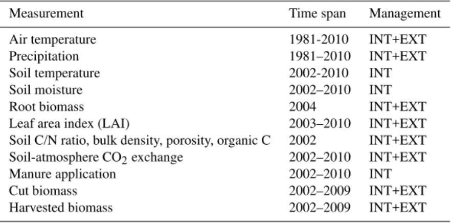
Table 2.Measurements taken in the context of the Oensingen experiments, used in this study (Ammann et al., 2007, 2009).
Measurement Time span Management
Air temperature 1981-2010 INT+EXT
Precipitation 1981–2010 INT+EXT
Soil temperature 2002-2010 INT
Soil moisture 2002–2010 INT
Root biomass 2004 INT+EXT
Leaf area index (LAI) 2003–2010 INT+EXT
Soil C/N ratio, bulk density, porosity, organic C 2002 INT+EXT
Soil-atmosphere CO2exchange 2002–2010 INT+EXT
Manure application 2002–2010 INT
Cut biomass 2002–2009 INT+EXT
Harvested biomass 2002–2009 INT+EXT
dynamics, uses few decomposition pools and a limited num-ber of input parameters. When compared to some of the more frequently used biogeochemical models, it resembles RothC and CENTURY rather than DNDC or PaSim. In contrast with RothC and CENTURY however, it maintains daily rather than monthly or annual integration steps. The development of a new model, moreover, allowed us to experiment with some alternative approaches.
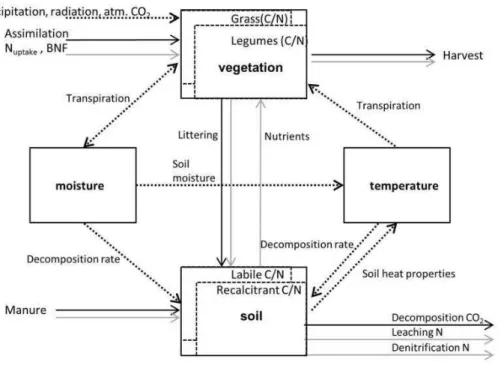
OGM simulates a soil-plant system in one spatial dimen-sion, with modules for temperature, moisture and C and N dynamics (Fig. 1). It uses three driving climatic variables (temperature, radiation, and precipitation), atmospheric CO2 concentration, 4 input parameters per soil layer (bulk den-sity, poroden-sity, C content and C:N ratio), 19 parameters that are specific for a vegetation type (e.g. water use efficiency, root/shoot turnover rate, specific leaf area), and 24 parame-ters that are site or soil type specific (e.g. potential decom-position rates, optimum decomdecom-position temperature, mois-ture, etc.). The latter, when describing soil properties, are as-sumed constant with soil depth. The OGM model uses daily averages for temperature and radiation, and daily sums for precipitation. The user can prescribe sub-daily time steps, however, to prevent numerical instabilities. Results presented here were obtained with an hourly time step. The model in-tegrates virtual soil layers, assuming constant conditions in each layer. The user can set the thickness of each layer de-pending on research interests and the availability of data. For the present simulations, the soil profile was divided into 11 layers (2×5 cm, 9×10 cm) to simulate a total soil depth of 1.0 m. OGM has a Microsoft Windows-specific (Visual C++) user interface which is separated from the model calculations that are ANSII compliant (C++).
2.2.1 Temperature and moisture
The temperature submodel is common to many soil biogeo-chemistry models; we will not describe it in detail here. A simple cascade approach was used to model soil moisture. The main processes that drive soil moisture are soil water
movement and uptake of soil moisture by the vegetation. Wa-ter movement depends on waWa-ter potentials that change with soil moisture in adjacent layers. Water uptake depends on soil moisture and root density. Further details of the water and temperature submodel can be found in M¨uller (2000).
2.2.2 Carbon and nitrogen balance
Plants can assimilate atmospheric CO2 and fix N2 through root symbiosis with rhizobia (Biological Nitrogen Fixation, BNF). The model treats organic manure-related additions of C and N (organic manure is always cattle slurry in INT) simi-lar to inputs of plant residues since it increases the decompo-sition pools according to concentrations of C, N and a frac-tion of manure that is labile.
While acknowledging that there is ongoing discussion about the biophysical interpretation of modeled decompo-sition pools, OGM conforms with models such as RothC, DNDC, COUP, or, CENTURY, by using conceptual rather than measurable decomposition pools, mainly in order to reduce the number of pools and to simplify model pa-rameterization (De Bruijn and Butterbach-Bahl, 2010; Par-ton et al., 1987; Li et al., 1992; Xu et al., 2011). OGM uses four decomposition pools, two for C and two for N distinguished according to decomposability (Clabile Nlabile, Crecalcitrant, Nrecalcitrant). Inorganic manure-bound N increases a separate pool of dissolved organic (DON) and inorganic (DIN) N (Ndisssl: DON+DIN in soil layer sl). Extraction of C and N occurs with harvests, net emission of CO2and ni-trogenous gases, or through leaching of Ndisssl. Leaching of DOC has not been investigated at the Oensingen field site, but Zeeman (2008) found that C leaching in a similar site in Switzerland was very small (0.05 t C ha−1yr−1).
Fig. 1.Overview of the Oensingen Grassland Model. The 4 solid-lined boxes are the main modules. The vegetation module can contain multiple plant functional types (here: grass and legumes in dotted boxes). The soil contains two decomposition pools, expressed in terms of C and N (dotted boxes). Arrows denote relationships between the modules. They can refer either to mass or information fluxes.
in the model. The OGM model uses plant functional types (i.e. categories of species with a similar growth strategy, phenotypical characterization, nutrient/moisture uptake ca-pacities, etc.) to deal with interspecies variability. Biochem-ical behavior of a functional type is described with uni-fied equations that can be parameterized differently. For the present simulations two plant functional types were used: legumes (v = 0) and grasses (v = 1). In the following, sub-scripts v, d, and sl are used to refer to individual vegeta-tion types {v = 0,1 for grass and legumes}, decomposition pools {d = 0,1 for labile and recalcitrant}, and soil layers
{sl = 0,slMax for increasing depth}.
Net ecosystem exchange (NEE) is the sum of CO2 assim-ilation and respiration:
NEE= 1 X
v=0
(δC
δt )assim,v−
1 X
d=0
(δC
δt)decomposition,d (1)
where (δCδt)assim,v is net assimilation by plant type v, and
(δCδt)decomposition,d is decomposition-related loss of C from decomposition pool d. Net biomass productivity (NBP) is the sum of C input and losses including management induced
changes:
NBP=NEE+(δC
δt)manure−
1 X
v=0
(δC
δt)harvest,v (2)
where(δCδt)harvest,vis biomass that is removed with harvests and (δCδt)manure is manure-bound C. All variables are ex-pressed in g C m−2. The N balance is calculated according to:
(δN
δt )system=
1 X
v=0
(δN
δt )BNF,v−( δN
δt )harvest,v)
(3)
+(δN
δt )manure−( δN
δt )emission−( δN
δt )leaching
where(δNδt)BNF,v is N fixation by v, (δNδt)harvest,v is N that is removed with harvest. (δNδt)manure is manure-bound N,
(δNδt )emission is N gaseous emission.(δNδt)leaching is N leach-ing. All variables are expressed in g N m−2.
2.2.3 Vegetation
AquaCrop, OGM uses crop transpiration as the main driver of assimilation:
(δC
δt )assim,v=Nsv×WUEv×(1.0+PCO2,v)×Trv (4)
where WUEvis the potential water use efficiency of v under current levels of atmospheric CO2(g C mm−1H2O), Nsvis a growth rate reduction factor that depends on the concentra-tion of N in leaves and Trvis transpiration by v. PCO2 is the
relative increase of WUE ( %) with increasing concentrations of atmospheric CO2:
PCO−2,v=
DCO−2,v 100% ×(
ρCO−2−370
370 ) (5)
where ρCO−2 is the concentration of atmospheric CO2 in ppm, DCO−2,vis the rate increase of photosynthesis in v if atmospheric concentration of CO2doubles compared to cur-rentρCO−2 = 370 ppm. Published estimates of DCO−2,vfor species in INT and EXT range from 20–40 % and estimates of individual species typically differ as much as those be-tween species (Aeschlimann et al., 2005; Ainsworth et al., 2003; Casella and Soussana, 1997; Ryle et al., 1992). In the present model applications, we used DCO2=33 % for both grasses and legumes (C3 plants) based on an extensive lit-erature review by Wand et al. (1999).
The N stress factor Nsvis calculated from foliage N ac-cording to
Nsv=(C2Nfv
C2N OPT,v)
λNsv (6)
where C2Nfvand C2NOPT,vare current and optimal C:N ra-tio in foliage of v,λNsv is a tuning parameter applied to v. Transpiration Trvin Eq. (4) is calculated from potential evap-otranspiration (ET0), which is estimated from air tempera-ture and radiation according to Priestley and Taylor (1972). Evaporation (E) and transpiration (T) are difficult to estimate in isolation. Some estimates given for example by Ham et al. (1990) suggest that T>>E in almost all stages of a de-veloping vegetation, which indicates that E from a developed canopy is very small. However, T equals zero by definition when LAI = 0, and a sharp decrease of E/ET0from 1.0 to 0.0 with increasing LAI is therefore necessary. Due to a lack of measurements of T, we are using the total leaf area in-dex LAItot (= 6LAIv) and we assume that E is negligible when LAItot>1.0 m2m−2(thus PTtot= ET0)and that PTtot = LAItot×ET0when LAItot<1.0. Some estimates indicate that this approximation may underestimate E with maximum 10 % when LAI∼1.0. In view of the magnitude of uncer-tainties we are dealing with in modeling biogeochemistry of a field site, we feel that this is acceptable (Ham et al., 1990; Saugier and Katerji, 1991; Merta et al., 2006).
PTvis derived from PTtotusing the dominance in foliage cover, domv= LAIv/LAItot, assuming that the capacity of a vegetation type to dominate water uptake of an ecosystem
with more than one type of vegetation (PTv/PTtot) corre-lates linearly with domv(PTv=domvPTtot). The actual tran-spiration of v (Trv)is estimated from PTvaccording to root biomass and moisture availability in individual soil layers:
Trv=
slMax X
sl=0
(frsl,v×( θsl−θwilt,v θporo−θwilt,v
)λsv
×PTv) (7)
where frsl,vis the fraction of root biomass of v in soil layer sl (see also Eq. 12), slMax is the number of soil layers and
θslis the water content in sl (VOL %),θwilt,vis soil moisture content at the level where v starts to wilt (VOL %),θporois water content at field capacity (VOL %) andλsvis a tuning parameter.
N uptake by plant roots is calculated according to:
(δN
δt )uptake,v=
slMax X
sl=0
Nupv×Ndisssl×frsl,v×Brv (8)
where Nupvis uptake capacity by roots of v (gN/gDW(root)), Brv = root biomass of v (gDWm−2). The OGM model as-sumes that BNF correlates linearly with root volume:
(δN δt )
= BNF,v
slMax X
sl=0
(BNFCv×frsl,v×Brv) (9)
where BNFCv is the rate of N2 fixation by roots of v (gN gDW(root)−1), with BNFCv= 0.0 when simulating species that are incapable of fixing atmospheric N2.
Two pools are used to describe vegetation development (Bs: shoot biomass and Br: root biomass; both in g DW m−2). The density of C in a component is a fixed parameter but the C:N ratio fluctuates. We are assuming that plants improve ac-cess to N by investing in roots when the C:N ratio in foliage increases, or vice versa, plants increase foliage biomass to improve assimilation of C when the C:N ratio drops (Thorn-ley and Johnson, 1990):
fCav=λCav×(C2NOPT,v
C2Ns ) (10)
where fCavis the fraction of assimilated C that is allocated aboveground, C2Nopt,v /C2Ns is shoot N status (capped to exclude values larger than 1.0) andλCavis a tuning param-eter. We further assume that foliage growth and N allocation does not depend on root C:N ratio, that aboveground alloca-tion of N (fNav: the fracalloca-tion of N that is allocated to above-ground parts) decreases as C2Ns drops below C2Nopt,v, and that roots are used to store excess N. For fNavwe used: fNav=1.0−λCbv×(C2NOPT,v
C2Ns ) (11)
at Oensingen suggest that this assumption tends to underes-timate root biomass in the top soil layer. Alternatively, we used:
Brv,sl=Brv× (D maxv/Dsl)
λBr
slMax P
sl=0
(D maxv/Dsl)λBr
(12)
where Brv,slis root biomass of v in sl, Brv is the total root biomass of v (gDWm−2), Dmaxv is rooting depth of vege-tation type v (m), Dslis the depth of soil layer sl (m), and parameterλBr is a shape parameter.
Foliage turnover (δBsδt )turnover,v depends on an intrinsic turnover rate which expresses the effect of ageing, and of water stress:
(δBs
δt )turnover,v=(TOfv+λsTOv×
TRv
PTv)×Bsv (13) where TOfvis reference foliage turnover rate andλsTOvis a shape parameter that increases foliage decay with water stress (m−1). Root biomass turnover(δBrδt )turnover,vis a con-stant fraction (TOrrvin kgDWkg−DW1)of root biomass:
(δBr
δt )turnover,v,sl=TOrv×Brv,sl (14)
The model assumes that harvest index (HI: extracted biomass/cut biomass) is constant regardless of harvesting method:
(δBs
δt )harvest,v=HI×( δBs
δt )cut,v (15)
The volume of cut biomass is estimated by subtracting the aboveground biomass that remains after a cut (Bivis derived from a vegetation specific parameter LAIinit,vthat is the LAI of v immediately after emergence) from biomass volume at the time of the cut (Bsv):
(δBs
δt )cut,v=(1.0−Biv)×Bsv (16)
The remaining biomass (cut but not removed) is added to the soil together with other residues:
(δC
δt )harv litter,v=( δBs
δt )cut,v−( δBs
δt )harvest,v (17)
where(δCδt)harv litter,vare biomass residues after a harvest. The current model structure cannot deal with grazing, which is not part of management systems applied at the Oensingen grasslands. Inclusion of grazing would require ad-ditional parameterization of cattle density and activity. We do expect however, that model performance in such setup would be lower due to spatial variability of manure additions which cannot be accounted for in a 1-D model.
2.2.4 Soil
Input of plant litter expressed in terms of C of v that is trans-ported to Cd(C0=Clabile, C1=Crecalcitrant)is expressed accord-ing to:
(δC
δt)litter,d,v=
slMax X
sl=0
(frv,sl×fd×ρCrv(δBrsl
δt )turnover,v) (18)
+fd×ρCsv(
δBs
δt )turnover,v+( δC
δt)harv litter,v
where frv,slis the fraction of root biomass of v in sl (derived from Eq. 12), fdis the fraction of labile (d=0) or recalcitrant (d=1) constituents in turnover biomass,ρCrvandρCsvare concentrations of C in root and shoot biomass (g C g−1DW). Additions to the N pools are expressed similarly, whereρNrv (calculated dynamically) is applied instead ofρCrv,ρNsv in-stead ofρCsv,δN/δt instead ofδC/δt.
The OGM user can specify manure applications as inor-ganic N (Ninorgin kgNha−1), organic N (Norgin kgNha−1), and organic C (Corgin kgCha−1). Organic manure enters a C pool according to:
(δC
δt)litter,d,sl=0=f md×( δC
δt )manure (19)
where fmd is the fraction of a component (d=0,1 for labile and recalcitrant) in applied manure. Additions to Ndare cal-culated with a similar equation (Ndfor Cd). Ninorgis added to Ndissslin the top layer (sl=0) of the soil:
(δNdiss
δt )litter,sl=0=( δN
δt )manure (20)
Decomposition of C from a pool Cdis calculated according to:
(δC
δt)dec,d,sl=Kd×τsl×msl×Cd,sl (21)
where Kd is the potential decomposition rate of d,τsl and
mslare temperature and moisture dependent reduction fac-tors for the decomposition rate. Decomposition of Nd is calculated with a similar equation by replacing Nd for Cd. The temperature-dependent rate reduction factor (τsl)is ex-pressed as:
τsl=Q (Tsl−10Topt)
10 (22)
where Q10 is the decomposition rate response to a 10◦C in-crease in temperature. Topt is the optimum decomposition temperature andTslis temperature of soil layer sl calculated in the temperature submodel (Fig. 1). The decomposition rate reduction factor associated with suboptimal soil mois-ture (msl)is expressed as:
msl=(
θsl
θopt
whereθslandθoptare soil water content in soil layer sl, and the optimum soil water content for decomposition, respec-tively, andλdec is a tuning parameter.
Leaching depends on the infiltration rate of moisture ac-cording to
(δNdiss
δt )leaching,sl=f×F wsl×
Ndisssl
hsl
(24) where (δNdissδt )leaching,sl is Ndiss that penetrates a deeper layer. Fwslis the rate of water infiltration in layer sl (m s−1), calculated in the water cycle module (Fig. 1), and f is a proportionality constant that expresses the fraction of N in Ndiss,sl that is mobile (i.e. nitrate/all species of dissolved N). Equation (24) quantifies leaching of N when sl = slMax. A constant fraction e of Ndiss is lost as gaseous emission
(δNδt)emission.
(δN
δt )emission,sl=e×Ndisssl (25)
Organic material slowly spreads due to bioturbation (i.e. mixing of material by soil animals). OGM assumes that the rate of transport of all litter types is equal, and decreases linearly with soil depth down to 1 m:
(δC
δt )pert,d,sl=cpert×(1.0−depthsl)×Cd,sl (26)
where Cd expresses a C decomposition pool (labile or re-calcitrant). Perturbation in the N pools (Nd for d={0,1}) is described with a similar equation by replacing Cd by Nd. Depthslis the distance from soil surface to the center of soil layer sl, and cpertis the rate of perturbation at the surface.
2.3 Model application
2.3.1 Initialization
Soil initial conditions for the top 0–60 cm in INT and EXT were derived from site-specific measurements of soil prop-erties (bulk density, organic carbon fraction, C:N ratio and porosity). These were used to initialize associated param-eters in the model (i.e. the model was not set to equilib-rium). An exponential fit was used to estimate soil proper-ties in 60–100 cm depth from available measurements above. Uncertainty limits of vegetation and model parameters were derived from published values, and tuning parameters were given uniform a-priori uncertainty ranges. Parameters such as altitude or heat properties of soil components remained fixed. We assumed that plant functional types (e.g. legumes and grasses) and site characteristics in INT and EXT were similar. Therefore, vegetation and model parameter values were equal.
2.3.2 Calibration
Uncertainty distributions were estimated for the different pa-rameters that were previously described. In the context of this
analysis, the use of a-priori knowledge was limited to esti-mates of minimum and maximum probable parameter val-ues that are presented in literature. The model was applied repeatedly where parameter values were changed with each model call. Note that a model call in this context consists of two simulations: INT and EXT. After each model call, the performance of the model was evaluated considering a suite of criteria, for which information is available (e.g. soil mois-ture, root biomass, LAI, etc.). This performance was given a score, that was calculated as the sum of the coefficient of variation of RMSE (CVRMSE= RMSE/(xmax−xmin), where RMSE =√(6(y–x)2/n), x = measured, y = modeled) over the criteria. The advantage of using CVRMSE as a perfor-mance quantifier is that it is unit independent and thus al-lows a comparison of multiple criteria. When we present op-timized model results, we are using parameter values that are associated with model calls that delivered the smallest value of 6CVRMSE in an extensive series (thousands) of model calls.
2.3.3 Evaluation
The model was evaluated using graphic comparisons of modeled and measured estimates. We further used some classic statistical parameters to describe goodness-of-fit of the model. For evaluation of individual measurement types, we have used normalized root mean square error (NRMSE) and coefficient of determination (R2). NRMSE (=RMSE/Xaverage)is similar to CVRMSE, but since it is more commonly used in scientific literature, NRMSE facilitates comparison with other publications.
2.3.4 Climate and management scenarios
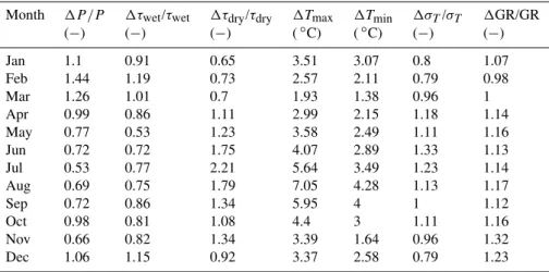
The climate change signal used to specify the scenarios was obtained from a simulation with the Climate High-Resolution Model (CHRM) (Vidale et al., 2003) completed in the framework of the PRUDENCE project (Christensen and Christensen, 2007). Corresponding changes in monthly precipitation amounts, average length of wet and dry spells, minimum and maximum temperature, temperature standard deviation, and solar radiation nominally valid for the end of the 21st century already given in Lazzarotto et al. (2010) are reproduced here in Table 3 for the sake of clarity.
Table 3.Changes (1)in monthly climate statistics between 2071–2100 and 1961–1990 (reference) simulated by the Climate High Resolution Model for the Swiss Plateau under the assumption of an A2 emissions scenario. Changes in mean precipitation rate (P), duration of wet (τwet)and dry (τdry)spells, global radiation (GR) and inter-annual standard deviation of air temperature (σT)are relative; changes in daily
maximum (Tmax)and minimum (Tmin)air temperature are absolute.
Month 1P /P 1τwet/τwet 1τdry/τdry 1Tmax 1Tmin 1σT/σT 1GR/GR
(−) (−) (−) (◦C) (◦C) (−) (−)
Jan 1.1 0.91 0.65 3.51 3.07 0.8 1.07
Feb 1.44 1.19 0.73 2.57 2.11 0.79 0.98
Mar 1.26 1.01 0.7 1.93 1.38 0.96 1
Apr 0.99 0.86 1.11 2.99 2.15 1.18 1.14
May 0.77 0.53 1.23 3.58 2.49 1.11 1.16
Jun 0.72 0.72 1.75 4.07 2.89 1.33 1.13
Jul 0.53 0.77 2.21 5.64 3.49 1.23 1.14
Aug 0.69 0.75 1.79 7.05 4.28 1.13 1.17
Sep 0.72 0.86 1.34 5.95 4 1 1.12
Oct 0.98 0.81 1.08 4.4 3 1.11 1.16
Nov 0.66 0.82 1.34 3.39 1.64 0.96 1.32
Dec 1.06 1.15 0.92 3.37 2.58 0.79 1.23
were adjusted using the anomalies specified in Table 3 (for details see Semenov, 2007). These adjustments were as-sumed to be valid in 2100; linear interpolation in time was internally applied to infer a transient evolution of the monthly climate (Lazzarotto et al., 2010).
Ultimately, 110 years of synthetic weather data were gen-erated for each scenario. In addition, a 110-year time se-ries was also generated without modification of the calibra-tion parameters. This simulacalibra-tion provides data statistically consistent with the current climate and was used in the so-called EQUIL runs (Table 4). We further used scenarios with changes in the precipitation regime during April to October (Growing Season Drought, GSD) or changes in precipitation, temperature and solar radiation (A2-370), both with atmo-spheric CO2concentration fixed at 370 ppm, and a scenario with changes in climate and CO2concentrations increasing to 860 ppm by 2100 (A2-860) according to predictions of at-mospheric CO2by the Bern-CC model for the A2 emission pathway (see Appendix I in IPCC, 2000).
Management events were forecast for each year in the pe-riod 2010–2100, by randomly picking a year between 2001 and 2010, and assuming that the recorded harvest/manuring events in this year are repeated in the forecast year. Combin-ing two management scenarios (INT/EXT) and four scenar-ios for climatic change (EQUIL/GSD/A2-370/A2-860), de-livered 8 model runs summarized in Table 4. Linear Regres-sion lines were fit to the last decade of soil C to determine sequestration, where soil C at 1 January 2001 and its fitted value in 2101 were used as indicators.
3 Results
3.1 Model evaluation and performance (2002–2010)
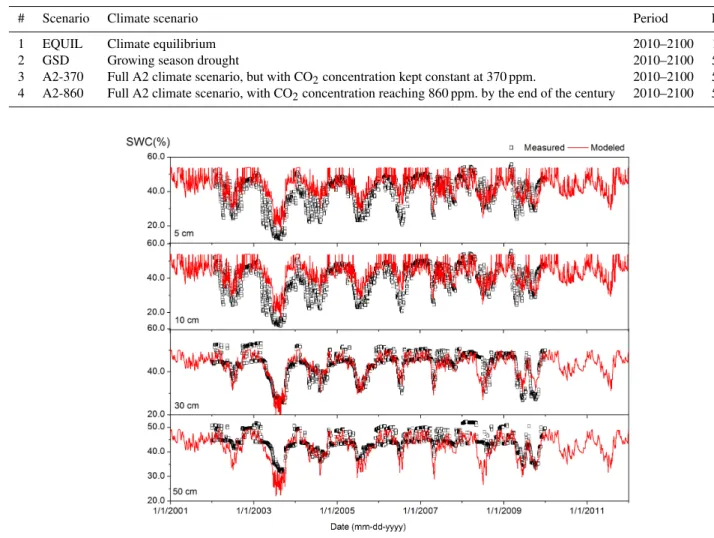
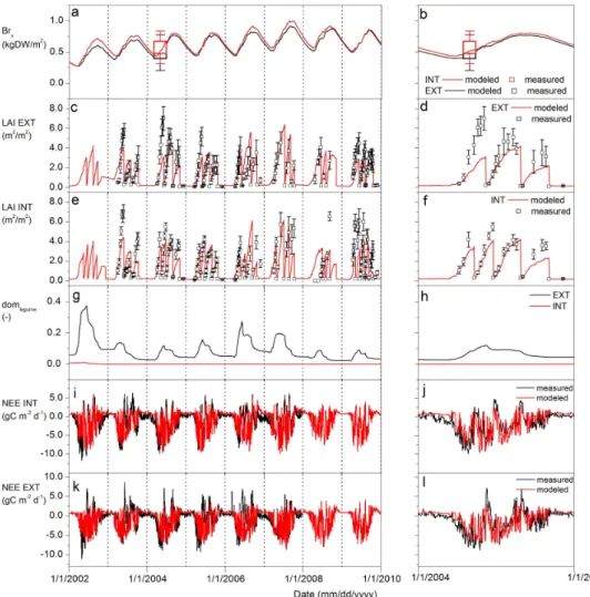
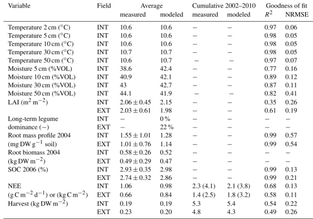
Coefficients of determination (R2)of soil temperature ranged from 0.97 to 0.99. Normalized root mean squared error (NRMSE) ranged from 0.05 to 0.07 (Table 5). Coefficients of determination (R2)of soil moisture ranged from 0.77 at 5 cm depth to 0.89 at 10 cm depth (Table 5; Fig. 2). NRMSE in-dicated a similar goodness of fit across different soil depths, with the best fit at 30 cm depth (NRMSE = 0.11), and the least fit at 50 cm depth (NRMSE = 0.41). Dry periods in the summers were usually well captured by the model. We did find, however, that the level of moisture extraction tended to be slightly underestimated in the top soil, while overesti-mated in deeper soil (compare 5 and 10 cm soil depth with 30 and 50 cm soil depth in Fig. 2).
According to the model simulation, legumes contributed
Table 4.Climate scenarios (reps. for randomized realizations of a climate scenario).
# Scenario Climate scenario Period Reps
1 EQUIL Climate equilibrium 2010–2100 1
2 GSD Growing season drought 2010–2100 5
3 A2-370 Full A2 climate scenario, but with CO2concentration kept constant at 370 ppm. 2010–2100 5
4 A2-860 Full A2 climate scenario, with CO2concentration reaching 860 ppm. by the end of the century 2010–2100 5
Fig. 2.Soil water content (SWC) expressed in %VOL in increasing soil depths.
Modeled root biomass approximated measured amounts in 2004 (Fig. 3; Table 5). Although not directly verified, there are indications that seasonal dynamics were plausible. For instance, Garcia-Pausas et al. (2011) measured maxi-mum seasonal fluctuations in grass root biomass of approxi-mately 30 % in a Pyrenees mountain grassland (compare with Fig. 3).
Aboveground litter production was 527– 585 g DW m−2yr−1 (EXT...INT), which was high com-pared to data of Hitz et al. (2001) who found values of 80–400 g C m−2yr−1 in grasslands that produce 100 to 300 g DW m−2 with individual harvests. Note that above-ground litter here does not include harvest remnants. Belowground litter production was 758–809 g DW m−2yr−1 (EXT...INT).
Turnover time of grass roots was 1.4 years, whereas Van der Krift and Berendse (2002) estimated root turnover times for some typical grass species (Lolium perenne, Arrhen-atherum elatius, Molinia caerulea, Nardus stricta) in the range from 0.8 to 1.11 years. Longer turnover times (3.3–
11.5 yr) were found in sub-alpine and alpine grasslands by Hitz et al. (2001).
3.1.1 Distribution of roots and soil C (2001–2006)
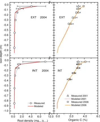
Root biomass in 2004 was slightly underestimated in EXT (modeled: 0.47 kg DW m−2; measured 0.49 kg DW m−2)
and in INT (modeled: 0.52 kg DW m−2; measured 0.58 kg DW m−2). It was particularly underestimated in the INT topsoil (0–5 cm, modeled: 5.9 mgDWg−soil1; measured 7.1±5.2 mgDWg−soil1), whereas root biomass density in the EXT topsoil (0–5 cm) was slightly overestimated (modeled: 5.3 mgDWg−soil1; measured 4.0±3.3 mgDWg−soil1). Note, however, that measurement errors in root biomass typically exceed the lack-of-fit of the model.
Fig. 3.Simulation and measurement results for grassland at Oensingen under extensive management (EXT) and intensive management (INT) at multi-annual (left panels) and annual (right panels) time scales.(a, b)measured and modeled sum of root biomass (Br, vertical bars indicate
±se);(c–f)measured and modeled LAI;(g, h)dominance of leguminous species in terms of foliage cover (domlegumes);(i–l)measured and
modeled net ecosystem exchange (NEE). Corresponding performance criteria are shown in Table 5.
Modeled carbon concentration had increased from 3.14 % to 3.85 % (EXT) and from 3.10 % to 4.04 % (INT) in the up-per 5 cm, from 3.15 % to 3.28 % (EXT) and from 3.05 % to 3.16 % (INT) between 5–10 cm depth. Small decreases were modeled in deeper layers (up to 0.14 %) in both INT and EXT with a maximum decrease at 10–20 cm depth. The dis-tribution of C across depth was well captured by the model (R2= 0.99, RMSE = 0.13–0.21 INT/EXT). Concentrations of C increased in the top 10 cm of soil, but decreased below 10 cm during 10 years of simulation.
3.1.2 Carbon balance (2001–2010)
The model was accurate for cumulative and inter-seasonal NEE in INT (Table 5), which indicated that the magni-tude of NPP, respiration, and cumulative NPP + respira-tion over time were simulated accurately. Cumulative CO2 fluxes were overestimated by 25 % in EXT. Harvests were
slightly underestimated in EXT but overestimated in INT. Soil in EXT started to lose C approximately 3 years after establishment. These losses had not stabilized in 10 years. Biomass reached a long-term average of 714 g DW m−2 in EXT (belowground biomass: 620 g DW m−2; aboveground biomass: 94 g DW m−2) and 751 g DW m−2 in INT (be-lowground biomass: 664 g DW m−2; aboveground biomass: 87 g m−2)after approximately 4 to 5 years (EXT and INT). Yet, stabilization of soil C was not completed until several decades in both INT and EXT (see Sect. 3.2.).
3.2 Carbon sinks in 2001–2100
Table 5.Model performance on soil, biomass, and carbon budget parameters for 2002–2010. Note that only pairs of modeled and measured values are included in cumulative and average values to facilitate comparisons. Sums of measured NEE, gap-filled with annual averages, are shown in brackets. Criteria for goodness of fit are given whenn >1.
Variable Field Average Cumulative 2002–2010 Goodness of fit
measured modeled measured modeled R2 NRMSE
Temperature 2 cm (◦C) INT 10.6 10.6 − − 0.97 0.06
Temperature 5 cm (◦C) INT 10.6 10.6 − − 0.98 0.05
Temperature 10 cm (◦C) INT 10.6 10.6 − − 0.98 0.05
Temperature 30 cm (◦C) INT 10.7 10.7 − − 0.98 0.05
Temperature 50 cm (◦C) INT 10.6 10.7 − − 0.97 0.07
Moisture 5 cm (%VOL) INT 38.6 42.4 − − 0.77 0.16
Moisture 10 cm (%VOL) INT 40.9 42.1 − − 0.89 0.12
Moisture 30 cm (%VOL) INT 43 42.7 − − 0.87 0.11
Moisture 50 cm (%VOL) INT 44.1 41.9 − − 0.82 0.41
LAI (m2m−2) INT 2.06±0.45 2.15 − − 0.35 0.26
EXT 2.03±0.61 1.98 − − 0.61 0.19
Long-term legume INT − 0 % − − − −
dominance (−) EXT − 22 % − − − −
Root mass profile 2004 INT 1.55±1.01 1.28 − − 0.99 0.57
(mg DW g−1soil) EXT 1.01±0.76 1.14 − − 0.99 0.54
Root biomass 2004 INT 0.58±0.26 0.52 − − − −
(kg DW m−2) EXT 0.49±0.29 0.47 − − − −
SOC 2006 (%) INT 2.93±0.35 2.98 − − 0.99 0.13
EXT 2.74±0.32 2.86 − − 0.99 0.21
NEE INT 1.06 0.98 2.3 (4.1) 2.1 (3.8) 0.68 0.13
(g C m−2d−1)or (kg C m−2) EXT 0.66 0.84 1.4 (2.5) 1.8 (3.2) 0.58 0.11
Harvest (kg DW m−2) INT 0.19 0.19 5.3 5.4 0.54 0.22
EXT 0.23 0.20 4.8 4.3 0.49 0.26
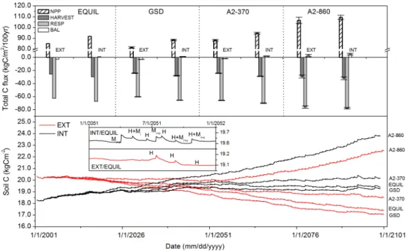
GSD/A2-370 scenarios and EQUIL occurred later. In EXT, losses of C were predicted to continue throughout the century and for all climate scenarios, except for A2-860, for which soil C loss stopped after 50 years and afterwards turned into an increase until the end of simulation. INT accumulated C during the first 45 years after establishment with all scenar-ios, and afterwards soil C remained nearly constant except for A2-860 where C accumulated throughout the century. Hence, towards the end of the simulation period, C dynam-ics were effectively dominated by vegetation responding to different climatic drivers.
Compared to EQUIL, NPP was lower in the GSD sce-nario (INT: −3.4 %, EXT: −4.4 %). NPP increased in the 370 scenario (INT: +3.1 %, EXT: +3.4 %) and in the A2-860 scenario as well (INT: +19.2 %, EXT: +25.2 %). Har-vested biomass was lower by a similar fraction in either man-agement system in the GSD scenario (INT:−5.4 %, EXT:
−5.2 %). Slightly higher harvests were predicted for the A2-370 scenario (INT: +3.1 %, EXT: +3.5 %), while consider-able increases were found for A2-870 (INT: +7.5 %, EXT: +14.2 %). Respiration decreased in the GSD scenario (INT:
−2.4 %, EXT:−3.4 %), but was higher in the other scenarios (INT/A2-370: +4.1 %, EXT/A2-370: +5.1 %, INT/A2-860: +7.5 %, EXT/A2-860: +14 %).
Net C sequestration over 100 years was predicted for all of the INT scenarios (EQUIL: +1.3 kg C m−2, GSD: +1.2±0.1 kg C m−2, A2-370: +1.8±0.2 kg C m−2, A2-860: +5.3±0.3 kg C m−2). Losses of soil C resulted for all EXT scenarios except A2-860 (EQUIL: −3.1 kg C m−2; GSD: −3.9±1.1 kg C m−2; A2-370: −2.1±0.3 kg C m−2, A2-860: +1.6±0.3 kg C m−2). Across all climate scenarios, there was a consistent and considerable difference between soil C sequestration in EXT and INT. Harvest and Respi-ration were tightly coupled to NPP in all the climate sce-narios, the ratio of harvest/NPP (in kg C/kg C) over the to-tal simulation period ranged from 27–30 % in EXT and 29– 32 % in INT (Fig. 5). Similarly, respiration/NPP ranged from 71–75 % in EXT and from 71–74 % in INT. Low respira-tion/NPP and harvest/NPP ratios were typically found for A2-860 in both INT and EXT. Highs were not so consistent, maximum harvest/NPP occurred in INT/EQUIL. Maximum respiration/NPP occurred in EXT/A2-370.
3.2.1 Distribution of roots and soil C in 2001–2100
-1.0 -0.9 -0.8 -0.7 -0.6 -0.5 -0.4 -0.3 -0.2 -0.1 0.0
0.0 2.0 4.0 6.0 12.0 -1.0
-0.9 -0.8 -0.7 -0.6 -0.5 -0.4 -0.3 -0.2 -0.1 0.0
0.0 2.0 4.0 6.0
2004
Organic C (%) INT
Soil depth (m)
EXT EXT
2004
Measured Modeled
Measured 2001 Modeled 2001 Measured 2006 Modeled 2006
Root density (mgDW/gSoil) INT
Fig. 4.Root density (left) and soil carbon concentration (right) for EXT (upper pane) and INT (lower pane). Measurements are given
±se.
between 15 and 80 cm depth (Fig. 4), summing up to
∼1.5 kg C m−2 over the entire 100-year simulation period. Hence, with time the range of depth, where soil C loss occurred, shifted slightly downward (compare Fig. 4 with Fig. 6).
4 Discussion
4.1 Long-term SOC
Our simulation results indicate that SOC stabilizes in EQUIL and GSD scenarios for INT, while C loss in EXT had not come to a halt in 2100.1SOC after land use conversion de-pends particularly on the balance of litter production, ma-nure application, and decomposition rates. Litter production depends on moisture and temperature, but also on seasonal aspects such as foliage cover, root density, growth, and har-vest efficiency. After a land use change, we can expect that litter production changes with growth rate. Decomposition of SOC depends foremost on a-biotic conditions, as well as quality and quantity of litter. SOC will therefore tend to in-crease or dein-crease depending on the new balance between litter fall and decomposition, until it stabilizes when the level
of SOC has changed to such extend that litter and manure input equals decomposition.
The level of SOC, at which saturation occurs, is of im-portance to explain our simulation results. We found relative changes in SOC of 7.0 % (INT) and−14.7 % (EXT), values that are lower than those given either by Poeplau et al. (2011) or IPCC (2000, table 1). While Poeplau et al. (2011) and IPCC (2000) review studies of lands that are exclusively managed in arable rotations, Oensingen had been under ley-arable management before conversion. Leifeld et al. (2005) found substantially higher SOC in ley-arable managed soil. The Oensingen sites contained 18–20 kg C m−2prior to con-version while IPCC (2000) assumes SOC = 8 kg C m−2 for croplands, and the arable soils considered by Poeplau et al. (2011) contained merely 4.6±2.1 kg C m−2. High SOC in ley-arable managed soil may be particularly due to high litter input in ley seasons. Because litter input may have been of similar quantity prior to land use change, sequestration po-tentials after conversion to permanent grassland may depend strongly on manure-C input (see also Sect. 4.2).
We can also compare our results with those found by Riedo et al. (2000), who modeled 3 sites with typical char-acteristics: Bern (high productivity), Sion (dry), and Davos (high altitude). The PaSim model was used to estimate se-questration potentials under different management options (cutting or grazing) and climates. Assuming a scenario comparable with our A2-860 scenario (lower precipitation, higher temperatures, radiation intensity and concentrations of atmospheric CO2; T2pm), Riedo et al. (2000) found that soil C decreased by∼5 % for Bern and∼10 % for Sion, but increased∼13 % for Davos, relative to a reference simulation (T0P0) that involved higher atmospheric CO2alone.
Our reference climate scenario (EQUIL) assumes that at-mospheric CO2 concentrations remain constant, so we ran an additional simulation using a climate scenario in which only atmospheric CO2increases, but temperature, precipita-tion and radiaprecipita-tion remain constant. We found lower C con-tents by 4.4 % in INT (0.8 kg C m−2)and by 4.8 % in EXT (1.0 kg C m−2)compared to the reference scenario, which is very similar to results of Riedo et al. (2000) for Bern.
Our estimate indicates an average sink of 0.05 kg C m−2yr−1in INT based on the difference between INT/EQUIL and EXT/EQUIL after 100 years. In compari-son, Lal et al. (2007) estimated that introducing fertilization creates a sink for C of only 0.01–0.02 kg C m−2yr−1 on average, or conversion of arable land to pasture, a sink of 0.04–0.06 kg C m−2yr−1. While our findings in INT are very comparable with studies reviewed in Lal et al. (2007), we found substantially lower sequestration potentials in EXT.
Fig. 5.Simulations of soil organic C (in g C m−2)between 2001–2100. Top panel: C budget 100 years after establishment of grassland. Bottom panel: Temporal C dynamics between 2001–2100 (inset: simulations of SOC between 2051–2052 for INT and EXT. Management activities are shown as H = harvest; Miand Mi+o= inorganic and organic plus inorganic manure application, respectively). Legend entries:
NPP = Net Primary Productivity, Harvest = extracted biomass, Resp = heterotrophic respiration, Bal = C balance (soil+biomass).
changes in SOC stock by sampling soil profiles over shorter time intervals (often directly after conversion).
We found that C accumulation initially occurs mainly in the top 10 cm of the soil, but increases to ∼15 cm in the course of the 100-year simulation. In agreement, Conant et al. (2001) found that SOC increments were observed partic-ularly in the top 10 cm soil. It is very common that SOC is not measured beyond 30 cm depth. In fact, the average soil depth in studies reviewed by Conant et al. (2001) was only 32.2 cm. However, we investigated how1SOC changes with soil depth (Fig. 6) and found indications that reliable assess-ments of C sequestration potentials need to consider deeper layers, as root biomass turnover increases with root depth. The change in SOC with depth is considerable in the top 50 cm of the soil at least, and the simulations suggest C loss to occur below 40 cm depth in the EXT/EQUIL scenario, and C gains above. Hence considerable changes in C sequestra-tion potentials can occur at levels deeper than are commonly measured, although depending on site management and his-tory, the potentials for C accumulation at>30 cm soil depth may be small.
4.2 The importance of biomass turnover and manure application
We found that C sequestration potentials differ considerably according to management intensity. In more detail, two pro-cesses are particularly important: biomass turnover and ma-nure application.
The assumption that vegetation characteristics for a co-hort (grass or clover) are the same regardless of management was inevitable because vegetation developments in INT and EXT would be equally well explained by plant characteris-tics (e.g. water use efficiency, biomass growth response to soil N) as by abiotic conditions (soil water content, dissolved N in the soil) if vegetation parameters had been allowed to vary freely. However inevitably, this assumption introduces some uncertainties. The seed mixture that was used in EXT, for example, contained different and more species of grasses than the mixture that was used in INT and also contained herbs.
Fig. 6.Simulated root density (left) and soil carbon (right) for EXT (upper pane) and INT (lower pane) in 2001 and 2100 under differ-ent climate and managemdiffer-ent scenarios. Measuremdiffer-ents in 2001 are given±se.
(0.44), whereas this ratio is nearly equal in the simulations (EXT: 0.37, INT: 0.40). The difference is consistent with a slight underestimation (0.1 kg C m−2) of soil C in 2006 in INT, and a considerable overestimation (1.0 kg C m−2)of modeled SOC in 2006 in EXT. Hence it is unlikely that this lack of fit is related to measurement uncertainty.
This finding is unexpected because litter in unfertilized (nitrogen poor) grassland is generally thought to decom-pose slower (Aerts et al., 2003). Instead a converse effect seems to dominate in EXT. For example, higher above-ground allocation could be sustained due to lower (below-ground) senescence. There are two known plant adaptations to nutrient poor conditions that lead to reduced senescence (Chapin, 1980; Louault et al., 2005). One response is instan-taneous: senescence of both root and shoot increases with protein concentration in the plant tissues. Moreover, root longevity may be extended due to mycorrhizal symbiosis that is stronger in nutrient poor conditions. A second response is genetic: slow-growing species are better capable to compete in nutrient poor conditions by increased longevity of biomass (Chapin, 1980).
Manure application increases soil C indirectly via higher plant assimilation and litter production as well as directly through manure-C amendment (Leifeld and Fuhrer, 2010;
Jones et al., 2006). We tested how these two mecha-nisms contribute to the difference that we found with four slightly different model applications. Excluding manure-derived C from our INT/EQUIL simulation (Table 4; i.e. only manure-N is spread among soil deposition pools according to Eq. 17) would lead to a 1.0 kg C m−2 lower soil C after 100 years (i.e. it reduces C increment from 1.1 kg C m−2to 0.1 kg C m−2). A similar difference is found when all manure-bound N is applied with inorganic fertil-izer (1SOC =∼0.0). The results indicate that∼60 % of the manure effect on soil C over a 100-year simulation can be attributed to import of C.
5 Conclusions
We have analyzed how management and global warming in-teract in two grassland systems established on former crop-land in Central Switzercrop-land. The aim was to investigate the long-term relationship between climate, soil C storage and management during a 100-year simulation period following establishment in 2002. The simulation results lead to the fol-lowing conclusions:
1. Intensive management (i.e. fertilization) drives the SOC dynamics until∼45 years after sowing, while cli-mate change determines soil C in the longer term. 2. Previous arable land use has to be specified exactly to
estimate potential sequestration of C. Prior to conver-sion, Oensingen grasslands had high SOC due to the use of ley-arable rotations as compared to an exclusively arable cropping system.
3. A larger fraction of the increase in soil organic C in fer-tilized plots originates from applied manure, compared to the input from increased amounts of plant litter. 4. After grassland establishment, soil C increases mainly
in the top 10 cm of soil, but in the course of 100 years, soil C increments are observed down to 15 cm.
5. Comparing the Oensingen site with conditions that are dominant in Switzerland, C sequestration potentials may be lower at warm low-precipitation sites, but higher at cooler and wet high-altitude sites.
Acknowledgements. This work was funded by the Swiss national Science Foundation in the framework of the NCCR Climate project AGRISK. We further thank Mikhail Semenov for the use of his LARS Weather Generator, as well as MeteoSwiss for making climate records publically available.
References
Aerts, R., De Caluwe, H., and Beltman, B.: Plant community medi-ated vs. nutritional controls on litter decomposition rates in grass-lands, Ecology, 84, 1398–3208, 2003.
Aeschlimann, U., N¨osberger, J., Edwards, T. J., Schneider, M. K., Richer, M., and Blum, H.: Responses of net ecosystem CO2 ex-change in managed grassland to long-term CO2enrichment, N
fertilization and plant species, Plant Cell Environ., 28, 823–833, 2005.
Ainsworth, E. A., Davey, P. A., Hymus, G. J., Osborne, C. E., Rogers, A., Blum, H., Nosberger, J., and Long, S. E.: Is stimu-lation of leaf photosynthesis by elevated carbon dioxide concen-tration maintained in the long term? A test with Lolium perenne grown for 10 years at two nitrogen fertilization levels under Free Air CO2Enrichment (FACE), Plant Cell and Environ., 26, 705–
714, 2003.
Ammann, C., Flechard, C. R., Leifeld, J., Neftel, A., and Fuhrer, J.: The carbon budget of newly established grassland depends on management intensity, Agric. Ecosyst. Environ., 121, 5–20, 2007.
Ammann, C., Spirig, C., Leifeld, J., and Neftel, A.: Assessment of the nitrogen and carbon budget of two managed temperate grass-land fields, Agric. Ecosyst. Environ., 133, 150–162, 2009. Casella, E. and Soussana, J.-F.: Long-term effects of CO2
enrich-ment and temperature increase on the carbon balance of a tem-perate grass sward, J. Exp. Bot., 48, 1309–1321, 1997.
Chapin, F. S.: The mineral nutrition of wild plants, Ann. Rev. Ecol. Syst., 11, 233–260, 1980.
Christensen, J. H. and Christensen, O. B.: A summary of the PRU-DENCE model projections of changes in European climate by the end of this century, Clim. Change, 81, 7–30, 2007.
Conant, R. T., Paustian, K., and Elliot, E. T.: Grassland manage-ment and conversion into grassland: effects on soil Carbon, Ecol. Appl., 11, 343–355, 2001.
Conant, R. T., Ogle, S. M., Paul, E. A., and Paustian, K.: Measuring and monitoring soil organic carbon stocks in agricultural lands for climate mitigation, Front Ecol. Environ., 9, 169–173, 2011. De Bruijn, A. M. G. and Butterbach-Bahl, K.: Linking carbon and
nitrogen mineralization with microbial responses to substrate availability – the DECONIT model, Plant Soil, 328, 271–290, 2010.
FAO, ISRIC and ISSS: World Reference Base for Soil Resources, Food and Agriculture Organization of the United Nations, Rome, 1998.
Garcia-Pausas, J., Casals, P., Romany`a, J., Vallecillo, S., and Se-basti`a, M.-T.: Seasonal patterns of belowground biomass and productivity in mountain grasslands in the Pyrenees, Plant Soil, 340, 315–326, 2011.
Gerwitz, A. and Page, E. R.: An empirical mathematical model to describe plant root systems, J. Appl. Ecol., 11, 773–782, 1974. Ham, J., Heilman, J. L., and Lascano, R. J.: Determination of soil
water evaporation and transpiration from energy balance and stem flow measurements, Agric. For. Met., 52, 287–301, 1990. Hitz, C., Egli, M., and Fitze, P.: Below-ground and above-ground
production of vegetational organic matter along a climosequence in alpine grasslands, J. Plant Nutr. Soil Sci., 164, 389–397, 2001. IPCC Intergovernmental Panel on Climate Change: Land use, land-use change and forestry, Cambridge, UK, Cambridge University Press, 2000.
IPCC: Climate Change 2007: The Physical Science Basis, Con-tribution of Working Group I to the Fourth Assessment Report of the Intergovernmental Panel on Climate Change, edited by: Solomon, S., Qin, D., Manning, M., Chen, Z., Marquis, M., Av-eryt, K. B., Tignor, M., and Miller, H. L., Cambridge University Press, Cambridge, UK and New York, NY, USA, 996 pp., 2007. Jenkinson, D. S., Adams, D. E., and Wild, A.: Model estimates of CO2emissions from soil in response to global warming, Nature, 351, 304–306, 1991.
Jones, S. K., Rees, R. M., Kosmas, D., Ball, B. C., and Skiba, U. M.: Carbon sequestration in a temperate grassland: management and climatic controls, Soil Use and Manage., 22, 132–142, 2006. K¨atterer, T., Reichstein, M., Andr´en, O., Lomander, A., and Andr´en, O.: Temperature dependence of organic matter decomposition: a critical review using literature data analyzed with different mod-els, Biol Fertil Soils, 27, 258–262, 1998.
Kesik, M., Ambus, P., Baritz, R., Br¨uggemann, N., Butterbach-Bahl, K., Damm, M., Duyzer, J., Horv´ath, L., Kiese, R., Kitzler, B., Leip, A., Li, C., Pihlatie, M., Pilegaard, K., Seufert, S., Simp-son, D., Skiba, U., Smiatek, G., Vesala, T., and Zechmeister-Boltenstern, S.: Inventories of N2O and NO emissions from
Eu-ropean forest soils, Biogeosciences, 2, 353–375, doi:10.5194/bg-2-353-2005, 2005.
Krift, T. A. J. van der and Berendse, F.: Root life spans of four grass species from habitats differing in nutrient availability, Funct. Ecol., 16, 198–203, 2002.
Kulshreshtha, S. and Sobool, D.: Comparative Greenhouse Gas Emission Intensities from Irrigated and Dryland Agricultural Ac-tivities in Canada, Canadian Water Res. J., 31, 157–172, 2006. Lal, R.: Carbon management in agricultural soils, Mitig. Adapt.
Strat. Global Change, 12, 303–322, 2006.
Lazzarotto, P., Calanca, P., Semenov, M., and Fuhrer, J.: Transient responses to increasing CO2and climate change in an unfertil-ized grass–clover sward, Climate Res., 41, 221–232, 2010. Leifeld, J. and Fuhrer, J.: Organic farming and soil carbon
seques-tration: What do we really know about the benefits? AMBIO, 39, 585–599, 2010.
Leifeld, J., Bassin, S., and Fuhrer, J.: Carbon stocks in Swiss agri-cultural soils predicted by land-use, soil characteristics, and alti-tude, Agric. Ecosyst. Environ., 105, 255–266, 2005.
Leifeld, J., Ammann, C., Neftel, A., and Fuhrer, J.: A comparison of repeated soil inventory and carbon flux budget to detect soil car-bon stock changes after conversion from cropland to grasslands, Glob. Change Biol., 17, 3366–3375, 2011.
Li, C., Frolking, S., and Frolking, T. A.: A model of nitrous oxide evolution from soil driven by rainfall events: 1. Model structure and sensitivity, J. Geophys. Res., 97, 9759–9776, 1992. Louault, F., Pillar, V. D., Aufr`ere, J., Garnier, E., and Soussana,
J.: Plant traits and functional types in response to reduced dis-turbance in a semi-natural grassland, J. Veg. Sci., 16, 151–160, 2005.
Merta, M., Seidler, C., and Fjodorowa, T.: Estimation of evaporation components in agricultural crops, Biom. and Life Sc., 61, 280– 283, 2006.
M¨uller, C.: Modelling Soil-Biosphere Interactions, CAB Interna-tional, 2000.
Poeplau, C., Don, A., Vesterdal, L., Leifeld, J., Wesemael, B. van, Schumacher, J., and Gensior, A.: Temporal dynamics of soil or-ganic carbon after land-use change in the temperate zone – car-bon response functions as a model approach, Glob. Change Biol., 17, 2415–2427, 2011.
Priestley, C. H. B. and Taylor, R. J.: On the assessment of surface heat flux and evaporation using large-scale parameters, Mon. Weather Rev., 100, 81–82, 1972.
Riedo, M., Grub, A., Rosset, M., and Fuhrer, J.: A pasture sim-ulation model for dry matter production, and fluxes of carbon, nitrogen, water and energy, Ecol. Model., 105, 141–183, 1998. Riedo, M., Gyalistras, D., and Fuhrer, J.: Net primary production
and carbon stocks in differently managed grasslands: simulation of site-specific sensitivity to an increase in atmospheric CO2and
to climate change, Ecol. Model., 134, 207–227, 2000.
Ryle, G. J. A., Weledge, J., Tewson, V., and Powell, C. E.: Influ-ence of Elevated CO2 and Temperature on the Photosynthesis and Respiration of White Clover Dependent on N22 Fixation,
Ann. Bot., 70, 213–220, 1992.
Saugier, B. and Katerji, N.: Some plant factors controlling evapo-transpiration, Agricultural and Forest Meteorology, Agr. Forest Meteorol., 54, 263–277, 1991.
Schimel, D. S.: Terrestrial ecosystems and the carbon cycle, Glob. Change Biol., 1, 77–91, 1995.
Semenov, M. A.: Development of high resolution UKCIP02-based climate change scenarios in the UK, Agric. For. Meteorol., 144, 127–138, 2007.
Steduto, P., Hsiao, T. C., Raes, D., and Fereres, E.: AquaCrop-The FAO crop model to simulate yield response to water: I Concepts and underlying principles, Agron. J., 101, 426–437, 2009. Thornley, J. H. M. and Johnson, I. R.: Plant and Crop Modeling,
Clarendon Press Oxford, 1990.
Van Wesemael, B., Paustian, K., Meersmans, J., Goidts, E., and Barancikove, G.: Agricultural management explains historic changes in regional soil carbon stocks, Proc. Natl. Acad. Sci. USA, 107, 14926–14930, 2010.
Vidale, P. L., L¨uthi, D., Frei, C., Seneviratne, S., and Sch¨ar, C.: Pre-dictability and uncertainty in a regional climate model, J. Geo-phys. Res., 108, 4586, 2003.
Wand, S. J. E., Midgley, G. F., Jones, M. H., and Curtis, P. S.: Re-sponses of wild C4 and C3 grass (Poaceae) species to elevated atmospheric CO2concentration: a meta-analytic test of current
theories and perceptions, Glob. Change Biol., 5, 723–741, 1999. Xu, X., Liu, W., and Kiely, G.: Modeling the change in soil organic carbon (SOC) of grassland in response to climate change: effects of measured versus modeled carbon pools for initializing RothC model, Agric. Ecosyst. Environ., 140, 372–381, 2011.