Phase Transitions in One-Dimensional
Nonequilibrium Systems
M. R. Evans
Department of Physics and Astronomy, The University of Edinburgh,
Mayeld Road, Edinburgh EH9 3JZ, U.K.
Received 1 November 1999
The phenomenon of phase transitions in one-dimensional systems is discussed. Equilibrium systems are reviewed and some properties of an energy function which may allow phase transitions and phase ordering in one dimension are identied. We then give an overview of the one-dimensional phase transitions which have been studied in nonequilibrium systems. A particularly simple model, the zero-range process, for which the steady state is known exactly as a product measure, is discussed in some detail. Generalisations of the model, for which a product measure still holds, are also discussed. We analyse in detail a condensation phase transition in the model and show how conditions under which it may occur may be related to the existence of an eective long-range energy function. It is also shown that even when the conditions for condensation are not fullled one can still observe very sharp crossover behaviour and apparent condensation in a nite system. Although the zero-range process is not well known within the physics community, several nonequilibrium models have been proposed that are examples of a zero-range process, or closely related to it, and we review these applications here.
I Introduction
In recent years the study of nonequilibrium systems has come to the fore in statistical mechanics. Basically, one can consider two types of nonequilibrium systems: those relaxing towards thermal equilibrium and those held far from thermal equilibriume.g. by the system being driven by some external eld. In the present arti-cle we will be mainly concerned with the latter scenario. To be more specic we dene our nonequilibrium systems as those evolving through a local stochastic dynamics which a priori does not obey detailed bal-ance, at least not with respect to any `reasonable' en-ergy function. The question of what is a reasonable energy function is a moot point. One might propose that the energy contains only local interactions, or is extensive, or is written down according to some physi-cal principles; but any answer to the question is subjec-tive. However, the basic point is that the nonequilib-rium system isdenedby its dynamics without regard to any concept of energy and it is the dynamics which should seem reasonable or `physical'. This is distinct from an equilibrium system where the energy function should be `physical' and the dynamics is usually dened in an ad hoc way simply to guarantee that one obtains the Gibbs-Boltzmann weight with the specied energy. The easiest way to do this is to use the detailed balance condition.
A natural way to construct a nonequilibrium steady state is to drive the system by forcing a current of some conserved quantity, for example energy or mass, through the system. Such systems are known as driven diusive systems (DDS). The archetypal model was in-troduced Katz, Lebowitz and Spohn [1]. Basically it comprises a two dimensional Ising-like lattice gas evolv-ing under conservative Kawasaki dynamics (spin ex-change) and with a drive direction imposed. It has been shown that a continuous phase transition exists in the driven system, as is also the case in the undriven (Ising) system, but, most interestingly, one seesgeneric long range (power-law decay) correlations as opposed to the undriven systems where long-range correlations are only seen at criticality. Although exact results are not available for this system[2], it is often thought that generic power-law correlations are related to the ex-istence of an eective long-range Hamiltonian for the system (see e.g. [3, 4]).
One intriguing feature of one-dimensional systems is the possibility of phase ordering and phase transi-tions. In recent years this possibility has begun to be explored and some examples are by now well studied. To appreciate the signicance one should recall the gen-eral dictum that in one-dimensional equilibrium sys-tems phase ordering and phase transitions do not oc-cur (except in the limit of zero-temperature, or with long range interaction|see Section II). In the one-dimensional nonequilibrium systems studied so far it appears that the presence of conserved quantities and an imposed drive are important in allowing ordering and phase transitions. However there still does not ex-ist a general theoretical framework within which to un-derstand the phenomena.
The purpose of this article is twofold. Firstly I wish to give a broad overview of phase transitions and phase ordering in one dimension|this is carried out in Section II. In particular, in Section II.1 we discuss the conditions under which ordering and phase transi-tions may occur in equilibrium systems i.e. the req-uisite properties of the energy function to allow such phenomena. Then in Section II.2 we catalogue some nonequilibrium, one dimensional systems which exhibit non-trivial phase behaviour
The second purpose is to discuss a very simple class of microscopic models, the zero-range processes [10, 11], which are presented in Section III.1. For these models the steady state can be calculated exactly since it fac-torises into a product measure. There is some irony in the fact that the system has found widespread applica-tion in the modellingof nonequilibriumphenomena (see Section VI), although the zero-range process was orig-inally introduced by Spitzer[10] as a dynamics which could lead to Gibbs measures. In Section IV we dis-cuss generalisations of the basic model which also have a product measure steady state. We show in Section V how the model can exhibit a phase transition, that we shall refer to as a condensation transition, which is anal-ysed in some detail. We also discuss an interesting sharp crossover phenomenon whereby models, although not fullling the conditions for strict condensation and phase ordering, may often appear to be in a condensed phase on a nite system. The simplicity of the system allows us to explore the roles of a conserved quantity, the presence of a drive and eective long-range energy functions. Conclusions are drawn in Section VII.
II Phase transitions in one
dimension
II.1 One-dimensional equilibrium
systems
As mentioned above, it is received wisdom that in one-dimensional equilibrium systems phase transitions do not occur. In fact any careful statement of this re-quires a few caveats and, indeed, a general rigorous
statement is hard to formulate (see [12] for a discus-sion).
Perhaps the best known argument is that of Landau and Lifshitz [13]. For simplicity, consider a one dimen-sional lattice ofLsites with two possible states, say A andB, for each site variable. Let us assume the ordered phases, where all sites take stateAor all sites take state B, have the lowest energy, and assume a domain wall (a bond on the lattice which divides a region ofAphase from that ofB) costs a nite amount of energy. Then n domain walls will cost energy n but the entropic contribution to the free energy due to the number or ways of placingn walls on L sites ' nT[ln(n=L),1] for 1 n L. Thus for any nite temperature a balance between energy and entropy ensures that the number of domain walls grows until it scales asL, that is, until the typical ordered domain size is nite.
Note that this argument relies on a nite energy cost for domain walls, and short range interactions so that one may ignore the interaction energy of domain walls. Indeed, the Ising model with long-range interac-tions decaying with distance asJ(r)r
,1, has been well studied [14] and it has been demonstrated that the one-dimensional system orders at low temperatures for 1 [15]. Also, of course we require non-zero tem-perature so that entropy comes into play, otherwise the two fully ordered states (ground states) would domi-nate the partition sum and the system would be frozen into them.
Another even simpler way of thinking of this is from a dynamical perspective. For a disordered state to or-der, domain walls must annihilate each other. However in one dimension no energy is gained by the two domain walls at opposite ends of a domain moving closer to one another; a domain always has two domain walls costing energy 2no matter what its size is. Therefore there is no eective force to eliminate domains and the system is disordered. Again, this argument requires a short range interaction so that one can ignore the energy of interaction of domain walls above some nite distance. A more mathematical way of addressing the ques-tion of phase transiques-tion in 1d is to use the transfer ma-trix technique [16]. For example, on a periodic one-dimensional homogeneous system ofN sites, the parti-tion sum can be written as the trace of a product ofN transfer matricesT :
Z= Trace
T N
=X
N (1)
whereare the eigenvalues of the transfer matrix. Now, since the transfer matrix is nite and the entries are all positive the Perron-Frobenius theorem [17] tells us that the largest eigenvalue max is non-degenerate. Thus, there can be no crossing of the largest eigenvalue as we vary some control parameter. Consequently the free energy F / lim
N!1(ln
Z)=N = max is analytic and we have no phase transitions (which would be signalled by some non-analyticity of the free energy).
This can occur when the transfer matrix becomes in-nite due, for example, either to long range interactions or when the local degree of freedom at each lattice site is not restricted to a nite number of statese.g. [18]. (An extreme instance of the latter case is when we are ac-tually considering a two dimensional system!) Another case when the Perron-Frobenius theorem does not ap-ply is when the transfer matrix becomes reducible i.e. when there exist components of T
N that are zero for all values of N. This can occur at zero temperature or when some interaction strengths are set to innity, an example being the rst order transition in the KDP model discussed in [19].
In this section we have discussed three arguments, presented here at dierent (low) levels of rigour, which all point to phase transitions in equilibrium one-dimensional systems only being possible in the case of long-range interactions, zero-temperature limit or in-nite interaction energies, or unbounded local variable at a site. As we shall see the situation for nonequilib-rium systems is less restrictive although some parallels can be drawn.
II.2 One-dimensional nonequilibrium
systems
Here we give an overview of one-dimensional sys-tems where phase transitions and phase ordering may occur. We focus our attention on hopping particle mod-els that, despite their simplicity, oer a wide range of non-trivial behaviour.
A simple one-dimensional model of a driven diu-sive system is the asymmetric simple exclusion process (ASEP). Here particles hop in a preferred direction on a one-dimensional lattice with hard-core exclusion (at most one particle can be at any given site). Indicating the presence of a particle by a 1 and an empty site (hole) by 0 the dynamics comprises the following exchanges at nearest neighbour sites
1 0 ! 0 1 with rate 1
0 1 ! 1 0 with rate q (2)
The open system was studied by Krug[20] and boundary induced phase transitions shown to be possi-ble. Specically one considers a lattice ofN sites where at the left boundary site (site 1) a particle is introduced with rateif that site is empty, and at the right bound-ary site (site N) any particle present is removed with rate. Thus the dynamical processes at the boundaries are
at site 1 0 ! 1 with rate
at siteN 1 ! 0 with rate : (3) These boundary conditions force a steady state current of particles J through the system. Phase transitions occur when limN!1
J exhibits non-analyticities. The steady state of this system was solved exactly for the to-tally asymmetric case [21, 22] and more recently for the
general qcase [23, 24]. Whenq<1 the phase diagram comprises three phases: a high-density phase where the current is limited by a low exit rate and takes the ex-pression J =(1,q,)=(1,q); a low-density phase where the current is limited by a low injection rate and takes the expression J = (1,q,)=(1,q); a maximal-current phase where both;>(1,q)=2 and the current is J = (1,q)=4. In the maximal current phase generic long-range correlations exist, an example being the decay of particle density from the left bound-ary to the bulk value 1=2 which is a power law1=x
1=2 where xis distance from the left boundary.
Clearly the presence of a conserved quantity and a drive, leading to non-zero current J is crucial to the phase transition. Indeed, the qualitative phase diagram appears robust for stochastic one-dimensional driven systems [25]. For the case of no bulk driveq= 1 [26, 27], or `reverse bias'q>1 [24] the current vanishes with in-creasing system size and there are no boundary-induced phase transitions.
The model has been generalised to two oppositely moving species of particle: one species is injected at the left, moves rightwards and exits at the right; the other species is injected at the right, moves leftwards and ex-its at the left [28]. Spontaneous symmetry breaking has been shown to occur, whereby for low exit rates () the lattice is dominated by one of the species at any given time. In the low limit the mean ip time between the two symmetry-related states has been calculated analytically and shown to diverge exponentially with system size [29].
In these models the open boundaries can be thought of as inhomogeneities where the order parameter (par-ticle density) is not conserved. Inhomogeneities which conserve the order parameter can be considered on a pe-riodic system. Indeed a single defect bond on the lattice (through which particles hop more slowly) is sucient to cause the system to separate into two macroscopic regions of dierent densities [30]: a high density region which can be thought of as a trac jam behind the defect and a low density region in front of the defect. Here the presence of the drive appears necessary for the defect to induce the phase separation.
Moving defects (i.e. particles with dynamics dier-ent from that of the others) have also been considered and exact solutions obtained [31, 32, 33, 34, 35]. In the model studied in [33, 34, 35], varying the rate at which the defect particle hops forward, denoted , and the rate at which it is overtaken and exchanges places with normal particles, denoted , produces a phase di-agram closely related to the open boundary problem. Moreover for low and highthere is a phase where the defect particle induces phase separation between a high density region behind it and a low density region in front of it.
the particle number and positions. It does not appear easy to relate this to any concept of an energy function. Indeed, it has been shown that a matrix product state is non-Gibbsian [37].
A natural question to ask is whether systems related to the hopping particle models described so far, but without inhomogeneities, can exhibit phase ordering. A very simple model was introduced in [38] comprising three species of conserved particles, amongst which all possible exchanges are allowed. However a key feature is that the dynamics has a cyclic symmetry. To be spe-cic let each site of a one-dimensional periodic lattice be occupied either by an A;B or C particle (there are no holes in this model). The dynamical exchanges are
AB ! B A with rate q B A ! AB with rate 1 B C ! C B with rate q C B ! B C with rate 1 C A ! AC with rate q
AC ! C A with rate 1 (4)
and we will takeq<1. For example, the hopping of an A particle is biased to the right when it is an environ-ment ofCs and it is biased to the left when it is in an environment ofBs.
The phase separation observed in the model is rather easy to understand: if the system has separated into a domain ofAs, followed by a domain of Bs, fol-lowed by a domain ofCs (in that order), then the do-main walls that are present AB,BC,CAare all stable objects. This is clear from (4) since, for example, anyA particles which penetrate the B domain will be driven backwards by the dynamics. On the other hand BA, CB or AC walls are all unstable objects and would be quickly eliminated by the dynamics.
In the special case of exactly equal numbers ofA;B and C particles it was shown that the model actually obeys detailed balance with respect to a long range asymmetric, energy function. In fact the energy is non-extensive in the sense that most congurations have energies of orderN
2[38]. The partition sum was calcu-lated in the large N limit (withq xed) and shown to depend linearly on N. This reects the fact that the phase separation is into three pure domains and the partition sum is dominated by the N equivalent trans-lations of the structure comprising three pure domains. When the numbers of particles are not identical, de-tailed balance does not hold but the phase separation into pure domains remains. Similar behaviour has been found in other related models with conserving dynamics [39, 40]. Another interesting model is where phase sepa-ration occurs on a quasi-one-dimensional system (2N sites) but not on a strictly one-dimensional system [41]. It should also be mentioned that systems with a cyclic symmetry but with non-conserving dynamics have been studied and shown to order into a frozen state [42].
Any discussion of nonequilibrium phase transitions is not complete without mentioning the most well
known class, that of directed percolation. Various mod-els are reviewed mod-elsewhere in this volume[43] so here I just sketch the basic behaviour by referring to a partic-ular model, the contact process [44, 45]. Each site of a lattice is either empty or contains a particle. Particles are annihilated with rate 1 and particles are created at empty sites with rate n=2 where n is the number of occupied nearest neighbours of the site (n = 0;1;2). Note that the `inactive state' where all sites are empty is an absorbing state. Above a critical value ofthere is a nite probability that starting from a single parti-cle on an innite lattice, the system will remain active ast!1. This phase transition has well-studied asso-ciated critical exponents and scaling behaviour. More-over it appears to be a universality class in the sense that the same exponents are found in all systems, with the same symmetry and conservation laws, exhibiting a phase transition from an absorbing inactive state to an active state[45].
However as described so far the contact process is distinct from the other hopping particle models dis-cussed in that on any nite lattice the absorbing state is reached in a nite time and is therefore the steady state. The active state only becomes available as a steady state on an innite system. We mention briey that it is in fact possible to dene hopping particle models, similar in spirit to the nonequilibrium models discussed in previous paragraphs, that exhibit phase transitions connected with directed percolation. These models can have non-conserved order parameter [46] or conserved order parameter [47]. Although there are no absorbing states in these models, they have the common feature of certain microscopic processes being forbidden.
A nal class of transitions in one-dimensional hop-ping particle models is that involving spatial conden-sation, whereby a nite fraction of the particles con-denses onto the same site. Examples include the ap-pearance of a large aggregate in models of aggregation and fragmentation[48] and the emergence of a single ock in dynamical models of ocking [49, 50]. In Sec-tion V we shall examine a very simple example of a condensation transition which occurs in the zero-range process and see how it is related to a defect induced transition.
III The zero-range process
The zero-range process was rst introduced into the mathematical literature as an example of interacting Markov processes [10]. Since then the mathematical achievements have been to prove existence theorems, invariant measures and hydrodynamic limits [44, 51].
model [54] for glassy dynamics due to entropic barri-ers; the drop-push model for the dynamics of a uid moving through backbends in a porous medium [55]; microscopic models of step ow growth [56, 57] and a bosonic lattice gas [58]. We shall discuss some of these in the sequel. The zero-range process is also closely re-lated to the more widely known asymmetric exclusion process [10, 44] as we shall describe below.
III.1 Model denition
In general one can consider the zero-range process on a lattice of arbitrary dimension, and of a (countably) innite or nite number of sites. Initially Spitzer [10] considered a nite number of sites. However, subse-quently most mathematical works tackle the invariant measure on an innite system [11]. For our purposes, it is most convenient to consider a nite system, com-pute the steady state and only then take the limit of an innite system. Note that the steady state t!1 and the innite volume limit do not necessarily com-mute e.g. on an innite system the invariant measure (steady state) is not necessarily unique.
We consider a one-dimensional nite lattice of M sites with sites labelled = 1:::M and periodic bound-ary conditions. Each site can hold an integer number of indistinguishable particles. The conguration of the system is specied by the occupation numbers n of
each site . The total number of particles is denoted by L and is conserved under the dynamics. The dy-namics of the system is given by the rates at which a particle leaves a site (one can think of it as the top-most particle|see Fig. 1a). As our rst example we assume it moves to the left nearest neighbour site ,1. The hopping rates u(n) are a function of n the number of particles at the site of departure. Some particular cases are: if u(n) = n then the dynamics of each parti-cle is independent of the others; if u(n) = const for n > 0 then the rate at which a particle leaves a site is unaected by the number of particles at the site (as long as it is greater than zero). It is helpful to think of
performing a Monte-Carlo simulation: in the u(n) = n case at each update a particle would be picked at ran-dom and moved to its nearest neighbour site; in the u(n) = constant case a site would be picked at random and a single particle moved to the nearest neighbour site.
A possible source of confusion in the denition of the model is that in [10] and some other papers the hop rates u(n) are dened as the hop rate perparticle at a site; thus u(n) in those works are 1=n of the u(n) dened here.
The important attribute of the zero-range process is that it yields a steady state described by a product measure. By this it is meant that the steady state prob-ability P(fng) of nding the system in conguration fn
1;n2:::nM
g is given by a product of factors f(n) often referred to as marginals
P(fng) = 1 Z(M;L)
M
Y
=1
f(n) : (5)
Here the normalisation Z(M;L) is introduced so that the sum of the probabilities for all congurations, with the correct number of particles L, is one. We shall explore later in Section V the interesting possibilities aorded by the form (5).
In the basic model described above, f(n) is given by f(n) = Yn
m=1 1
u(m) for n1
= 1 for n = 0 (6)
Note that f(n) is dened only up to a multiplicative constant and we could have included a factor znin (6).
Later this factor reappears as a fugacity in Section V. The proof of (5,6) is, happily, straightforward. One simply considers the stationarity condition on the prob-ability of a conguration (probprob-ability current out of the conguration due to hops is equal to probability current into the conguration due to hops):
c X
(n)u(n)P(n1:::n:::nL) = X
(n)u(n+ 1+1)P(n1:::n ,1;n
+1+1:::nL) : (7) We have included the Heaviside function to highlight that it is the sites with n > 1 that allow exit from the conguration (lhs of (7)) but also allow entry to the conguration (rhs of (7)). Equating the terms with > 1 and cancelling common factors assuming (5), results (for n1) in
u(n)f(n,1)f(n) = u(n+1+ 1)f(n
,1)f(n
+1+ 1) (8)
This equality can be recast as
u(n) f(nf(n )
,1) = u(n
+1+ 1)f(n
+ 1+ 1)
f(n+1) = constant
Setting the constant equal to unity implies f(n) = f(n,1)
u(n) (10)
and iterating (10) leads to (6) where we have chosen f(0) = 1.
Figure 1. Equivalence of zero range process and asymmetric exclusion process.
III.2 Relation to the asymmetric
exclusion process
There exists an exact mapping from a zero-range process to an asymmetric exclusion process. This is il-lustrated in Fig. 1. The idea is to consider the particles of the zero-range process as the holes (empty sites) of the exclusion process. Then the sites of the zero-range process become the moving particles of the exclusion process. This is possible because of the preservation of the order of particles under the simple exclusion dy-namics. Note that in the exclusion process we have M particles hopping on a lattice of M + L sites
An interesting feature of the mapping is that it con-verts a model where the local degree of freedom can take unbounded values (particle number in the zero-range process) to a model where the local site variable is restricted to two values. On the other hand, a hop-ping rate u(m) which is dependent on m corresponds to a hopping rate in the exclusion process which depends on the gap to the particle in front. So in principle the particles can feel each other's presence and it is possible to have a long-range interaction.
IV Generalizations
We now show how the totally asymmetric, homoge-neous zero-range process we have considered so far may be generalised yet retain steady states of a similar form to (5,6).
IV.1 Inhomogeneous system
First we consider an inhomogeneous system by which we mean the hopping rates are site dependent: the hopping rate out of site when it contains n
par-ticles is u(n). It is easy to check that the steady state
is simply modied to P(fng) =
1 Z(M;L)
L
Y
=1
f(n) : (11)
where f are given by
f(n) = Yn
m=1 1
u(m) for n1
= 1 for n = 0 (12)
The proof is identical to that given above for the ho-mogeneous case, with the trivial replacement of u(n)
by u(n)
IV.2 Discrete Time Dynamics
A further generalisation is to the case of discrete time dynamics. This has been studied in [59] in the context of a disordered asymmetric exclusion process. Here we translate the results into the zero-range pro-cess. Rather than processes occurring with a rate, time is counted in discrete steps and at each time step events occur with certain probabilities.
In the case ofParallel Dynamics, at each time-step all sites are updated. One particle from each site is moved to the left, each with probability p(n) where
nis the number of particles at the site before the
up-date. Note that the particles move simultaneously and particles do not move more than one site.
It turns out that the steady state again has the form (11). It was shown in [59] that
f(n) = 1,p(1) for n = 0 = 1,p(1)
1,p(n)
n
Y
m=1
1,p(m)
p(m) for n > 0 :
(13) To recover the continuous time dynamics we can call the interval between time steps dt and let p(n) =
u(n)dt. Then continuous time dynamics is given by
the limit dt!0 and, to within a constant factor dtn, (13) recovers (12). In this way one can interpolate be-tween discrete time, parallel dynamics and continuous time dynamics.
forwards and backwards updating sequences were de-rived and it turns out they too have the form (11) with ftaking an expression related to the parallel case (13).
IV.3 Arbitrary Network
In the original paper paper of Spitzer[10] some more general versions of the zero range process were consid-ered. Here we discuss one interesting case which serves to generalise the (totally asymmetric) zero range pro-cess dened above to a propro-cess on a more general lattice or for any nite collection of points with a prescribed transition matrix for the dynamics of a single particle [11].
In this case the rate of hopping of a particle at site containing n particles is equal to u(n) and the
probability that a particle leaving site will move to site is denoted W(!). Thus the probability that in time dt a particle at moves to is
u(n)W(!) dt : (14) Note that the probabilities W(!) dene a stochastic matrix for a single particle moving on a nite collection of M sites and we take
X
W(
!) = 1 : (15)
so that probability is conserved. We refer to the collec-tion of points together with the prescribed transicollec-tion matrix W(!) as the network.
We assume that the transition matrix is irreducible (i.e. the particle can pass from any given point to any other after sucient time and the system is ergodic) so that we have a unique steady state probability for the single particle problem:
s=X
sW(
!) : (16)
We now show that the steady state for the many-particle problem dened above is given by (11) where now f(n) is given by
f(n) = Yn
m=1
s
u(m)
for n1
= 1 for n = 0 (17)
The proof is again a straightforward generalisation of that of Section III. Equation (7) is modied to
c X
(n)u(n)P(n1:::nL) = X
X
6=
(n)p(!)u(n+1)P(n
1:::n+1:::n
,1:::nL) : (18) Equating the terms on each side of (18), assuming (11) and cancelling common factors yields
(n)u(n)f(n) = (n)X
6=
W(!)u(n+1)f(n,1)f
(n+1)
f(n) : (19)
d Inserting (17) leads to the condition
s=X
6=
sW(!) (20)
which is the same as the single particle steady state condition (16).
A simple case considered by Spitzer is when W(!) is a doubly stochastic matrix which is dened by the property
X
W(
!) = X
W(
!) = 1 : (21) Equations (21) and (16) then imply that the single par-ticle problem has a homogeneous steady state s =
con-stant.
Let us also discuss an example where the single par-ticle problem has an inhomogeneous steady state. We
consider a one-dimensionallattice where hops to the left and right neighbours are allowed but with probabilities that depend on the site. Thus, we may write
W(!) = q for = + 1 (22)
= 1,q for = ,1 (23)
= 0 otherwise : (24)
The steady state of the single particle problem (random walker on a disordered one dimensional lattice [60])
s= (1,q
+1)s+1+ q,1s,1 (25) can be solved and one obtains
s=
"
M,1 X
i=0 1 q,i
i
Y
=0 q, 1,q
, #
: (26)
The sites in the present model correspond to the parti-cles in the exclusion process which each have their own forward and backward hopping rates. Another, par-ticular instance of this network occurs in [52], where
a repton model of gel electrophoresis is studied in the case of periodic boundary conditions (see Section VI).
In special cases of the zero-range process detailed balance may hold. The condition for this is
c u(n)W(
!)P(n
1:::nL) = u(n+ 1)W(
!)P(n
1:::n+1:::n
,1:::n
L) : (27)
Substituting the form (11,17) leads to the condition
d
sW(
!) = s
W(
!) (28)
which is just the detailed balance condition for the sin-gle particle problem.
An interesting consequence of the form of the steady state (17) is that it allows one to relate an arbitrary zero-range process to a model obeying detailed balance. The idea is that if detailed balance doesn't hold, we can always dene a new zero-range process (to be denoted by a prime) with the same steady state, but with a dif-ferent dynamics obeying detailed balance. To do this, we solve the single particle problem (16) for the original model to obtain s. For any collection of points we can always dene a new single particle transition matrix W0(
!) that satises detailed balance with respect to a homogeneous steady state (s0
= constant). The new model is dened by a new set of hopping rates u0
(m) = u (m)s
0 =s
together with the new transition matrix W0(
!). It is easy to check from (17) that the new model has the same steady state as the original.
Thus, within the realm of zero-range processes, to the steady state of any nonequilibrium model we can always identify a model satisfying detailed balance and therefore an energy function. Of course, although the steady states are the same, there is no reason for the dynamical behaviour of the two systems to be related. To clarify this point we will discuss a simple example
in Section .
The marginals (17) have the interesting structure of being a product of a term (s)
n that depends on the nature of the network and a term involving the product of u(m) which reects the interactions at the site. The network can represent an arbitrary dimensional lattice or the eects of disorder, the only diculty to surmount in obtaining the steady state is the solution of the single particle problem.
V Condensation Transitions
We now proceed to analyse the steady states of form (11) and the condensation transition that may occur. The important quantity to consider is the normalisa-tion Z(M;L) as it plays the role of the partinormalisa-tion sum. The normalisation is dened through the condition
Z(M;L) = X
n1;n2:::nM
(X
n
,L) M Y =1
f(n) (29) where the function enforces the constraint of L parti-cles. The normalisation may be considered as the ana-logue of a canonical partition function of a thermody-namic system.
We dene the `speed' v as the average hopping rate out of a site
c
v = Z(M;L)1 X
n 1
;n 2
:::n M
(X
n
,L)u(n 1)
M Y =1
f(n) = Z(M;L,1)
Z(M;L) (30)
d where we have used (11,12). Note that (30) tells us that the speed is independent of site and thus may be considered a conserved quantity in the steady state of the system. In the totally asymmetric system consid-ered in Section III.1 the speed is equal to the current
obey-ing detailed balance the (net) current is zero, but the speed as dened above remains nite. The speed is a ratio of partition functions of dierent system sizes (30)
and corresponds to a fugacity, as we shall see below. We will consider also the probability distribution of the number of particles at a site, taken here to be site 1 c
P1(n1= x) = 1 Z(M;L)
X
n2:::nM
(x + n2+ :::nM ,L)f
1(x)
M
Y
=2 f(n)
= f1(x)Z(M
,1;L,x)
Z(M;L) (31)
d (where Z(M,1;L,x) is the partition function for a system with site 1 removed). In general the probability distribution is site dependent but for a homogeneous system (f independent of ) it will be the same for all
sites.
We now use the integral representation of the delta function to write the partition function as
Z(M;L) =I dz
2i z,(L+1)
M
Y
=1
F(z) ; (32)
where
F(z) =
1 X
m=0
zm f(m) : (33)
For large M;L (32) is dominated by the saddle point of the integral and the value of z at the saddle point is the fugacity. The equation for the saddle point reduces to
L M = Mz
M
X
=1 @
@z lnF(z) (34)
which, dening = L=M, can be written as = zM XM
=1 F0
(z)
F(z) : (35)
In the thermodynamic limit,
M !1 with L = M ; (36)
where the density is held xed, the question is whether a valid saddle point value of z can be found from (35). We expect that for low the saddle point is valid but, as we shall discuss, there exists a maxi-mum value of z and if at this maximaxi-mum value the rhs of (35) is nite, then for large (35) cannot be satis-ed. We now consider separately, and in more detail, how condensation may occur in the inhomogeneous and the homogeneous case.
V.1 Inhomogeneous case
In general, the inhomogeneous casei.e. where F(z) depends on the site through (17), is dicult to anal-yse. Here we would just like to give an idea of how a condensation transition may occur by discussing a sim-ple examsim-ple. We then go on to analyse perhaps the simplest example of a condensation transition: a single inhomogeneous site [62].
First we take the general model discussed in Sec-tion IV.3 and set u(m) = u for m > 0 i.e. the hopping rate does not depend on the number of parti-cles at a site. We consider doubly stochastic transition matrices W(!) (see Eq. 21) so that we may take s() = constant and without loss of generality we set the constant equal to one. For the moment we do not specify further the transition matrix; later we will dis-cuss two specic examples one obeying detailed balance and one not. Under these conditions f is given by
f(n) =
1 u
n
(37)
and the probability of occupancies fn
1;n2;:::;nM gis P(fn
1;n2;:::;nM g) =
1 Z(M;L)
M
Y
=1
1 u
n
: (38)
The mapping to an ideal Bose gas is evident: the L particles of the zero-range process are viewed as Bosons which may reside in M states with energies E
Bose gas. We can sum the geometric series (33) to ob-tain F
and F
0
then taking the large
M limit allows the sum over to be written as an integral
= Z
1 umin
duP(u) z u,z
(39) where P(u) is the probability distribution of site hop-ping rates with umin the lowest possible site hopping rate. Interpreting P(u) as a density of states, equation (39) corresponds to the condition that in the grand canonical ensemble of an ideal Bose gas the number Bosons per state is. The theory of Bose condensation [64] tells us that when certain conditions on the density of low energy states pertain we can have a condensa-tion transicondensa-tion. Then (35) can no longer be satised and we have a condensation of particles into the ground state, which is here the site with the slowest hopping rate. This case is discussed further, in the context of an asymmetric exclusion process on an innite system, by J. Krug in this volume [65].
We now turn to the simplest case of an inhomoge-neous system: site 1 hasu1=pwhile the otherM,1 particles have hopping rates u
= 1 when
>1. It is easy to see that (11) simplies to
P(fn
g) = 1 Z(M;L)
1 p
n1 (40)
In this case the normalisationZ(M;L) is easy to cal-culate combinatorially:
Z(M;L) =
X n1;n2:::nM
( X
n
,L)p
,n1
= L
X n1=0
L+M,n1,2 M,2
p
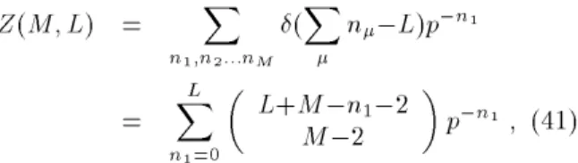
,n1 ; (41) yielding an exact expression for the speed through (30). In the thermodynamic limit the sum (41) is dominated by n1 O(1) for < p=(1,p) and n1 O(L) for >p=(1,p) and it can be shown that
c
for < p 1,p
Z(M;L)'
L+M M
1 1+
p
p,(1,p) and
v!1, (42)
for > p 1,p
Z(M;L)'p ,L(1
,p)
,(M,1) and
v!=(1 +) (43)
d In the high density phase, dened by (43) we have a condensate since the average number of particles at site 1 is hn1i=L =,p=(1,p). In the low density phase (42) the particles are evenly spread between all sites and we will refer to it as the homogeneous phase.
We now discuss two models which both have this steady state: a driven system and a system obeying de-tailed balance. This provides an illustration of the idea discussed in Section IV.3 whereby a zero range process not obeying detailed can be related to one obeying de-tailed balance.
First we take the totally asymmetric model so that particles move to the site to the left: the transition matrix is
W(!) = ;,1
:
So this model is similar to that discussed in Sec-tion III.1, and a mapping to a totally asymmetric ex-clusion process can be made in the same way as Sec-tion III.2. The equivalent exclusion process is illus-trated in Fig. 2. We see that the equivalent exclusion process is system of hard-core particles hopping to the right, one particle being slower than the rest. The in-terpretation of the two phases within the context of the exclusion process is that in the condensed phase (for the exclusion process a low density of particles) a `trac
jam' forms behind the slow particle and the slow par-ticle has a nite fraction of the lattice as `empty road' ahead. Whereas in the homogeneous phase (a high den-sity of particle for the exclusion process) the particles are roughly evenly spaced.
Figure 2. A totally asymmetric exclusion model (upper) and a model with zero current (lower) that have equivalent steady states leading to (41).
On the other hand one may consider the case where the one particle problem is a symmetric random walk so that the system obeys detailed balance. The transition matrix is given by
W(!) = 12
;,1+ 12
When we map this system to a simple exclusion pro-cess we see from Fig. 2 that we have a system of parti-cles, the bulk of which perform a symmetric exclusion dynamics but with two adjacent asymmetric particles: the left one biased to the left and the right one biased to the right. In the condensed phase the gap between these particles diverges. Previously a single asymmetric particle in a sea of symmetric particles has been studied [66] but in that case there is no phase transition. At rst it seems that we have found a counterexample to the received wisdom that no phase transition should occur in an equilibrium system, since we have a condensation transition in a model with local dynamics obeying de-tailed balance. Inferring an energy function from the steady state (40) through the following equation
exp[,(E)] = exp[,(x 2
,x 1)lnp]
reveals that our eective energy increases linearly with distance x2
,x
1between the two asymmetric particles. Therefore the energy is `unphysical' in that it has very long range interactions. Thus the phase transition can be rationalised within the categories of exceptions dis-cussed in Section II.1.
We have seen that this simplest example of a con-densation transition (a single inhomogeneous site in the zero range process) is exhibited both in a driven model and also in a model obeying detailed balance but with long-range energy function. Again it should be stressed that although the steady states of these two models are equivalent, the dynamical properties should be very dierent. For example in the homogeneous phase of the driven model we expect asymmetric exclusion like behaviour and the dynamic exponent should be 3=2 implying relaxation times of M3=2 on a nite system. However in the homogeneous phase of the model obey-ing detailed balance we expect symmetric exclusion like behaviour and the dynamic exponent to be 2 implying relaxation times of M2 [67].
V.2 Homogeneous case
We now consider the homogeneous zero-range pro-cess where in (14) the hopping rates are site indepen-dent and the single particle problem (16) has a homoge-neous steady state s = 1 [68]. A similar analysis has
been carried out in the context of balls-in-boxes and branched polymer models [69].
In the present case, (33) is independent of and reads
F(z) = 1 X
n=0
n
Y
m=1
z u(m)
(44) The fugacity z must be chosen so that F converges or else we could not have performed (33). Therefore z is restricted to z where we dene to be the radius of convergence of F(z). From (44) we see that is the limiting value value of the u(m) i.e. the limiting value of the hopping rate out of a site for a large number of
particles at a site. We interpret (35) as giving a rela-tion between the density of holes (number of holes per site) and the fugacity z. The saddle point condition (35) becomes
= zF0(z)
F(z) (45)
Given that the rhs of (45) is a monotonically increasing function of z (which is not dicult to prove) we deduce that density of particle increases with fugacity. How-ever if at z = , the maximum allowed value of z, the rhs of (45) is still nite then one can no longer solve for the density and one must have a condensation tran-sition. Physically, the condensation would correspond to a spontaneous symmetry breaking where one of the sites is spontaneously selected to hold a nite fraction of the particles.
Thus, for condensation to occur (i.e. when is large enough for (45) not to have a solution for the allowed values of z) we require
lim
z! F0(z)
F(z) <1: (46)
We now assume that u(n) decreases uniformly to in the large n limit as
u(n) = (1 + (n)) (47)
where (n) is a monotonically decreasing function. Analysis of the series
F() = 1
X
n=0 exp
( ,
n
X
m=1
ln[1 + (m)] )
F0() = 1 X
n=0 nexp
( ,
n
X
m=1
ln[1 + (m)] )
(48) reveals that the condition for condensation is simply that F0() is nite and this occurs if u(n) decays to more slowly than (1 + 2=n). (This is easiest to see by expanding ln[1 + ] and approximating the sum over m by an integral in (48).)
In order to t this result into the picture of Section Section II.1 one can argue that since the condensate has an extensive number of particles at a site, the local site variable is unbounded. Therefore the `no phase tran-sition rule' does not apply. One also gains insight by translating the results into the language of the simple exclusion process. In this context we can have conden-sation if the hop rate of a particle into a gap of size n decays as (1+2=n) therefore there is an eective long range interaction.
V.3 Sharp crossover phenomena
where, although there is no strict condensation transi-tion, some interesting crossover phenomena occur [68].
Consider
u(n) = 1 for n<r (49)
u(n) = for nr: (50)
One can interpret these hop rates as meaning that a site only distinguishes whether it contains greater than r particles. When we use the mapping of Section III.2 to a totally asymmetric exclusion processrbecomes the
range of the interaction in the sense that it is the num-ber of sites ahead up to which a particle in the exclusion process distinguishes.
When these hopping rates are inserted in (44) one obtains
F(z) = r ,1 X n=0 z
n+ 1 X n=r z
n
r , n,1
: (51)
Performing the geometric series readily yields c
F(z) = 1 ,z
r 1,z
+ z
r ,z
(52)
zF 0(
z) = z
1,z r (1,z) 2
, r z
r ,1 1,z
+ z
r (,z)
2 + r z
r , 1 (,z)
: (53)
Then we nd the condition (45) can be written after a little algebra as (,z)
2[
,z(1 +)] = z r(1
,)[(1+,2z)z,(1,z)(,z)] +r z
r(1
,z)(,z)(1,) (54)
Therefore for larger we nd the solutions for <
1,
z' 1+
,r
1+
r
1,
(1+)(, (1+)) (55)
for = 1,
z',
(1+r )=3(1
,) (56)
for > 1,
z', (1+r )=2
1, (, (1+))
1=2 (57)
d
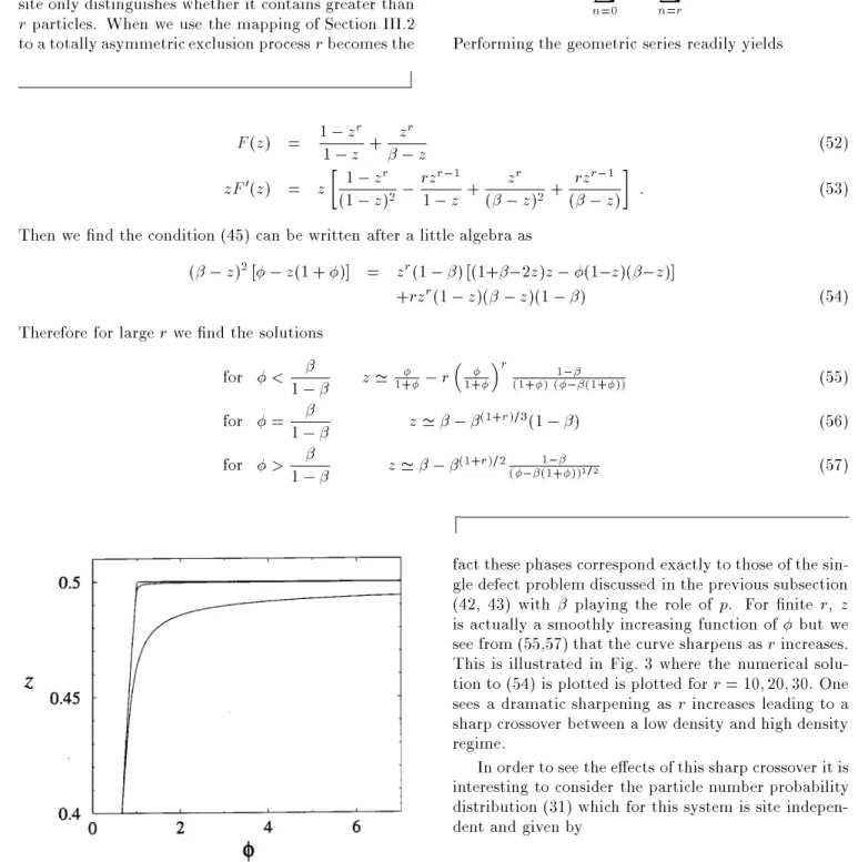
Figure 3. Solutions to (54) for =0:5and r =10;20;30 (increasing insharpness ofcurve).
Thus we see asr !1we have two phases: a high den-sity phase > =(1,) where the speed is and a low density phase where the speed is =(1 +). In
fact these phases correspond exactly to those of the sin-gle defect problem discussed in the previous subsection (42, 43) with playing the role of p. For nite r, z is actually a smoothly increasing function of but we see from (55,57) that the curve sharpens asrincreases. This is illustrated in Fig. 3 where the numerical solu-tion to (54) is plotted is plotted forr= 10;20;30. One sees a dramatic sharpening as rincreases leading to a sharp crossover between a low density and high density regime.
In order to see the eects of this sharp crossover it is interesting to consider the particle number probability distribution (31) which for this system is site indepen-dent and given by
P(x) z x for
x<r (58)
(z=) x for
xr: (59)
distribution for largex>rgoes as P(x)exp
,x
(1+r )=2 1 , (,(1 +))
1=2
(60) so that the typical occupancy of well-occupied sites goes as
,r =2. Taking, for example
= 0:1 andr= 10 leads to a typical occupancy of10
5. Therefore to simulate the model one requires a number of particles very much larger than this! If care is not taken to do this, and the total number of particles in the system is comparable to the typical occupancy, one would have an apparent condensate on a nite system.
An example of this phenomenon was studied re-cently within the context of a `bus route model' [70]. There the underlying motivation was to consider how a non-conserved quantity could mediate an eective long-range interaction amongst a conserved quantity in a driven system with a strictly local dynamical rule. The model considered was dened on a 1d lattice. Each site (bus-stop) is either empty, contains a bus (a con-served particle) or contains a passenger (non-concon-served quantity). The dynamical processes are that passengers arrive at an empty site with rate ; a bus moves for-ward to the next stop with rate 1 if that stop is empty; if the next stop contains passengers the bus moves for-ward with rateand removes the passengers. Since the buses are conserved, there is a well dened steady state average speed v. This fact can be used to integrate out the non-conserved quantity (passengers) within a mean-eld approximation. The idea is that a bus stop, next to bus 1 say, will last have been visited by a bus (bus 2) a mean time ago of n=v where n = x
2 ,x
1 is the distance between bus 2 and bus 1. Therefore the mean-eld probability that the site next to bus 1 is not occupied by a passenger is exp(,n=v). From this probability an eective hopping rate for a bus into a gap of size nis obtained by averaging the two possible hop rates 1;:
u(n) =+ (1,)exp(,n=v): (61) We can now see that this mean-eld approximation to the bus-route model is equivalent to a homoge-neous zero-range process as discussed earlier in this section. Since u(n) decays exponentially, with decay length r =v =, the condition for a strict phase tran-sition is not met. It is reasonable to believe that the system behaves in a similar way to the system with a nite `range'rdiscussed in Section V.3. Sincercan be made arbitrarily large as!0, on any nite system an apparent condensation will be seen. In the bus route problem this corresponds to the universally irritating situation of all the buses on the route arriving at once.
VI Some further applications
As mentioned earlier the zero-range process and related models have appeared several times in the modelling of
nonequilibrium phenomena. Here we briey discuss a few of these instances to illustrate the ubiquity of the basic model.
In [53] models of sandpile dynamics are considered. A zero range process is used to model the toppling of sand on a one-dimensional lattice; specically the sys-tem is homogeneous and the occupation number of a site becomes the height of sand (h) at that site. The hopping rates are set as u(1) = 1 and u(h) = for h > 1, with the transition matrix a symmetric ran-dom walk, and the limit of large considered. This limit means that a particle (grain of sand) keeps mov-ing until it nds an unoccupied site, thus a hoppmov-ing event may play the role of an avalanche. (Although in terms of sandpiles and self-organised criticality this model is rather trivial, it did serve to investigate the idea of a diverging diusion constant.) Note that a slightly dierent !1 limit (where the direction of the initial move of the particle is maintained until it nds an unoccupied site) was also considered but the product measure is still retained.
In a dierent context Barma and Ramaswamy [55] introduced the `drop-push' model of activated ow in-volving transport through a series of traps. Each trap can only hold a nite number of particles. For the trap depth set equal to one this model is essentially the same as the sandpile model of [53] discussed above (i.e. it is a zero-range process with some innite rates). In fact the version studied in [71] is precisely the limitofu(n)!1 forn>1 of the totally asymmetric zero-range process described in Section III.1. A generalisation to inhomo-geneous traps, and partially asymmetric hopping rates dependent on the occupancy of the trap was made in [72] and a steady state similar to (11,17) demonstrated. The zero-range process is also relevant in the con-text of 1+1 dimensional interface growth by the step ow mechanism. The interface can be visualised as an ascending staircase of terraces. Adatoms land on the terraces and diuse until they bind to the ascending step. If the ratio of deposition rates over diusion rates tends to zero then the resulting dynamics is that a race shrinks by one unit (and the adjacent higher ter-race grows by one unit) with a rate proportional to the size of the terrace. Thus the terrace lengths are equiva-lent to the site occupancies of an asymmetric zero-range process that was discussed in Section III.1. The equiv-alence of zero range processes to a general class of step ow models is discussed in [57].
inhomo-geneities in site hopping rates reect the shape of the polymer tube.
VII Conclusion
In this work the aims were to give an overview of the area of phase transitions and ordering in one-dimensional systems and also to analyse in some detail a particularly simple model, the zero-range process. In Section II several features were identied which could lead to the anomalous behaviour of ordering and phase transitions in equilibrium systems: long-range interac-tions; zero temperature; unbounded local variable. For nonequilibrium systems some concepts which may be important emerged: conserved order parameter; drive; forbidden microscopic transitions.
The simplicity of the zero-range process allowed us to analyse the steady state of the model in detail. First we derived the steady state for a general class of zero-range processes in Sections III and IV. We then anal-ysed the condensation transitions that can occur. On an inhomogeneous system the condensation is very rem-iniscent of Bose-Einstein condensation. For it to oc-cur requires certain conditions to hold on the distribu-tion of hopping rates. In the homogeneous system the condensation corresponds to a spontaneous symmetry breaking, since an arbitrary site is selected to hold the condensate. The condition for it to occur is that the hopping rate dependence on the site occupancy decays suciently slowly. It was also shown that when the condition for condensation does not hold, one can still observe very sharp crossover behaviour and apparent condensation on a nite system
An interesting possibility that was explored was that of the existence of an eective energy function. We saw that any steady state of the form (11,17) can be obtained from a process obeying detailed balance. However when the eective energy is inferred for cases where phase transition occurs (as was carried out for an explicit example in Section V.3) we nd that it con-tains long-range interactions. Thus the condensation transition can be rationalised within the equilibrium framework.
Moreover in the zero-range process the existence of a drive or preferred direction, producing a conserved particle current, is not essential for the occurrence of a condensation transition. What does appear neces-sary, however, is the conservation of particles. The xed number of particles implies implies the introduction of a fugacity z through (32), which in turn controls the condensation transition. As we saw the fugacity gives the hopping rate out of a site (referred to as speed in Section V) which is a conserved quantity.
On the other hand, for other models the presence of a preferred direction and conserved current does seem crucial for the existence of phase transitions. For
exam-ple, the asymmetric exclusion process dened in Sec-tion II.2 has non-trivial phase behaviour but the un-driven version (symmetric exclusion) does not.
In summary, although a general theoretical frame-work for the description of phase transitions in one di-mensional systems is not yet available, we hope that the issues and models discussed in the present paper serve to show that our understanding is developing.
Acknowledgements
Some of the work described here, particularly in Sec-tion II.2, has been the outcome of many enjoyable col-laborations over the years and I thank all of my collabo-rators warmly. Special thanks are due to Owen O'Loan who kindly allowed me to borrow from parts of his PhD thesis in Sections V.2 and V.3 and with whom I have enjoyed many enlightening discussions. I also thank Isao Hiyane for pointing out the KDP model to me and Richard Blythe, Deepak Dhar and Joachim Krug for helpful comments on the manuscript.
References
[1] S. Katz, J. L. Lebowitz and H. Spohn Phys. Rev. B
28, 1655 (1983); J. Stat. Phys.34, 497 (1984).
[2] B. Schmittmann and R. K. P. Zia (1995) Statistical Mechanics of Driven Diusive Systems, edited by C. Domb and J.L. Lebowitz (Academic Press, U.K., 1995), Vol. 17; B. Schmittmann and R. K. P. Zia, Phys. Re-ports301, 45 (1998).
[3] B. Bergesen, Z. Racz and H-J Xu, Phys. Rev. E52,
6031 (1995).
[4] F. J. Alexander and G. L. Eyink, Phys. Rev. E57,
R6229 (1998).
[5] J. Krug, Adv. Physics46, 139 (1997).
[6] For an overview see Trac and Granular Flow `97, edited by M. Schreckenberg and D. E. Wolf (Springer, Singapoure, 1998).
[7] K. Heckmann,Passive permeability of cell membranes, biomembranes(New York, Plenum Press, 1972) Vol. 3, p. 127.
[8] T. Chou and D. Lohse, Phys. Rev. Lett. 82, 3552
(1999).
[9] C.T. MacDonald, J.H. Gibbs and A.C. Pipkin, Kinetics of biopolymerization on nucleic acid templates Biopoly-mers61{25 (1968).
[10] F. Spitzer, Advances in Math.5, 246 (1970).
[11] E. D. Andjel, Ann. Probability10, 525 (1982).
[12] E. H. Lieb and D. C. Mattis,Mathematical Physics in One Dimension: Exactly Soluble Models of Interacting Particles(Academic Press, London, 1966), Chapter 1. [13] L. D. Landau and E. M. Lifshitz,Statistical Physics I
[14] M. E. Fisher, S.-k. Ma and B. G. Nickel, Phys. Rev. Lett.29, 917 (1972).
[15] F. J. Dyson, Commun. Math. Phys.12, 91 (1969).
[16] N. Goldenfeld, Lectures on Phase Transitions and the Renormalization Group(Addison Wesley, 1985). [17] S. Karlin and H. M. Taylor,A First Course in
Stochas-tic Processes(Academic, New York, 1975); F. R. Gant-macher,Matrix Theory(Chelsea, 1959) Vol. II, Chapter XIII.
[18] J.M.J van Leeuwen and H.J. Hilhorst, Physica A107,
319 (1981).
[19] J. F. Nagle, Am. Journal of Physics36, 1114 (1968).
[20] J. Krug,Phys. Rev. Lett.67, 1882 (1991).
[21] B. Derrida, M. R. Evans, V. Hakim and V. Pasquier, J. Phys. A26, 1493 (1993).
[22] G. Schutz and E. Domany, J. Stat. Phys. 72, 277
(1993).
[23] T. Sasamoto, J. Phys. A 32, 7109 (1999);
cond-mat/9910270.
[24] R. A. Blythe, M. R. Evans, F. Colaiori and F. H. L. Essler (1999) cond-mat/9910242
[25] A. B. Kolomeisky, G. M. Schutz, E. B. Kolomeisky and J. P. Straley J. Phys. A31, 6911 (1998).
[26] R. B. Stinchcombe and G. M. Schutz, Europhys. Lett.
29, 663 (1995).
[27] T. Sasamoto, S. Mori and M. Wadati, J. Phys. Soc. Japan65, 2000 (1996).
[28] M. R. Evans, D. P. Foster, C. Godreche, D. Mukamel, Phys. Rev. Lett.74, 208 (1995).
[29] C. Godreche, J-M. Luck, M. R. Evans, D. Mukamel, S. Sandow and E. R. Speer, J. Phys. A28, 6039 (1995).
[30] For a review see S. A. Janowsky and J. L. Lebowitz, in Nonequilibrium Statistical Mechanics in One Di-mension, edited by V. Privman (Cambridge University Press, U.K., 1997) Chapter 13, and references therein. [31] B. Derrida, S.A. Janowsky, J.L. Lebowitz, E.R. Speer,
J. Stat. Phys.73, 813 (1993).
[32] Z. Toroczkai and R. K. P. Zia, Phys. Lett. A217, 97
(1996).
[33] K. Mallick, J. Phys. A29, 5375 (1996).
[34] B. Derrida and M. R. Evans, J. Phys. A 32, 4833
(1999).
[35] T. Sasamoto, (1999) cond-mat/9910483. [36] B. Derrida, Phys. Reports.301, 65 (1998).
[37] E. R. Speer, in Micro, Meso and Macroscopic Ap-proaches in Physics, edited by C. Maes and A. Ver-beure (Plenum, 1994).
[38] M. R. Evans, Y. Kafri, H. M. Koduvely and D. Mukamel, Phys. Rev. Lett. 80, 425 (1998); Phys.
Rev. E58, 2764.
[39] P. F. Arndt, T. Heinzel and V. Rittenberg, J. Phys. A
31, L45 (1998); cond-mat/9809123.
[40] R. Lahiri, M. Barma, S. Ramaswamy (1999) cond-mat/9907342.
[41] G. Korniss, B. Schmittmann and R. K. P. Zia, Euro-phys. Lett.45, 431 (1999).
[42] L. Frachebourg, P. L. Krapivsky and E. Ben-Naim, Phys. Rev. E54, 6186 (1996).
[43] H. Hinrichsen (2000). This volume.
[44] T. M. Liggett,Interacting Particle Systems(Springer, Berlin, 1985).
[45] J. Marro and R. Dickman,Nonequilibrium Phase Tran-sitions in Lattice Models(Cambridge University Press, Cambridge, 1991).
[46] U. Alon, M.R. Evans, H. Hinrichsen and D. Mukamel (1996) Phys. Rev. Lett.76, 2746 (1996).
[47] D. Helbing, D. Mukamel and G.M. Schutz, Phys. Rev. Lett.82, 10 (1999).
[48] S. N. Majumdar, S. Krishnamurthy, M. Barma (1998) Phys. Rev. Lett.81, 3691 (1998); cond-mat/9908403.
[49] A. Czirok, A-L. Barabasi, T. Vicsek, Phys. Rev. Lett.
81, 209 (1999).
[50] O. J. O'Loan and M. R. Evans, J. Phys. A 32, L99
(1999).
[51] H. Spohn (1991), Large Scale Dynamics of Interacting Particles, (Springer-Verlag, New York, 1991).
[52] J.M.J van Leeuwen and A. Kooiman, Physica, A184,
79 (1992).
[53] J. M. Carlson, E. R. Grannan and G. H. Swindle, Phys. Rev. E,47, 93 (1993).
[54] F. Ritort, Phys. Rev. Lett.75, 1190 (1995).
[55] M. Barma and R. Ramaswamy in Non-linearity and Breakdown in Soft Condensed Matter, edited by K.K. Bardhan, B. K. Chakrabarti and A. Hansen (Springer, Berlin, 1993) p. 309.
[56] J. Krug and M. Schimschak, J. Phys I France,5, 1065
(1995).
[57] J. Krug, in Nonequilibrium Statistical Mechanics in One Dimension, edited by V. Privman (Cambridge University Press, U.K., 1997), chapter 15.
[58] R. Kutner, K. W. Kehr, W. Renz and R. Przenioslo, J. Phys. A,28, 923 (1995).
[59] M. R. Evans, J. Phys. A,30, 5669 (1997).
[60] B. Derrida, J. Stat. Phys.31, 433 (1983).
[61] I. Benjamini, P. A. Ferrari, C. Landim, Stoch. Proc. Appl.61, 181 (1996).
[62] M. R. Evans, Europhys. Lett.36, 13 (1996).
[63] J. Krug and P. A. Ferrari, J. Phys. A,29, L465 (1996).
[64] For a clear exposition see e.g. K. HuangStatistical Me-chanics, 2nd edition (Wiley, New York, 1987). [65] J. Krug (2000). This volume.
[66] S. F. Burlatsky, G. Oshanin M. Morea and W. P. Rein-hardt, Phys. Rev. E54, 3165 (1996).
[67] L. H. Gwa and H. Spohn, Phys. Rev. A46, 844 (1992).
[69] P. Bialas, Z. Burda and D. Johnston, Nucl. Phys. B
493, 505 (1997).
[70] O. J. O'Loan, M.R. Evans and M.E. Cates, Phys. Rev. E58, 1404 (1998).
[71] G. M. Schutz, R. Ramaswamy and M. Barma, J. Phys. A29, 837 (1996).
[72] G. Tripathy and M. Barma, Phys. Rev. E , 1991 (1998).
[73] M. Rubinstein, Phys. Rev. Lett.59, 1496 (1987); T. A.