Zero-inflated Poisson regression models for QTL mapping applied to tick-resistance in a Gyr x Holstein F2 population

Zero-inflated Poisson regression models for QTL mapping

applied to tick-resistance in a Gyr x Holstein F2 population

Fabyano Fonseca Silva

, Karen P. Tunin

, Guilherme J.M. Rosa

, Marcos V.B. da Silva

,

Ana Luisa Souza Azevedo

, Rui da Silva Verneque

, Marco Antonio Machado

and Irineu Umberto Packer

_{Departamento de Estatística, Universidade Federal de Viçosa, Viçosa, MG, Brazil.}

2

_{Departamento de Zootecnia, Universidade de São Paulo. Piracicaba, SP, Brazil.}

_{Department of Animal Science, University of Wisconsin, Madison, WI, USA.}

Empresa Brasileira de Pesquisa Agropecuária, Centro Nacional de Pesquisa de Gado de Leite,

Juiz de Fora, MG, Brazil.

Abstract

Nowadays, an important and interesting alternative in the control of tick-infestation in cattle is to select resistant ani-mals, and identify the respective quantitative trait loci (QTLs) and DNA markers, for posterior use in breeding pro-grams. The number of ticks/animal is characterized as a discrete-counting trait, which could potentially follow Poisson distribution. However, in the case of an excess of zeros, due to the occurrence of several noninfected ani-mals, zero-inflated Poisson and generalized zero-inflated distribution (GZIP) may provide a better description of the data. Thus, the objective here was to compare through simulation, Poisson and ZIP models (simple and generalized) with classical approaches, for QTL mapping with counting phenotypes under different scenarios, and to apply these approaches to a QTL study of tick resistance in an F2 cattle (Gyr x Holstein) population. It was concluded that, when working with zero-inflated data, it is recommendable to use the generalized and simple ZIP model for analysis. On the other hand, when working with data with zeros, but not zero-inflated, the Poisson model or a data-transfor-mation-approach, such as square-root or Box-Cox transformation, are applicable.

Key words:dairy cattle, tick infestation, QTL regression, generalized linear model.

Received: March 29, 2011; Accepted: July 22, 2011.

Introduction

In the tropics, cattle can be afflicted by various tick species and the diseases they transmit, possibly leading to significant loss in production systems. Among these, Rhipicephalus (Boophilus) microplusis outstanding. Apart from the reduction in production, infection can even be mortal to more susceptible animals.

Regarding losses caused by Boophilus microplus, Frischet al.(2000) estimated that an animal with an aver-age of 40 ticks per day could lose weight equivalent to 20 kg/year, whereas Furlonget al.(1996) calculated a re-duction of 23% in the daily milk yield, when crossbred Hol-stein-Zebu cows were infested by 105 ticks, on an average. Thus, the control of infestation is of extreme importance for the dairy and beef industries.

An important and interesting alternative in the control of tick infestation in cattle is to select resistant animals, and identify those specific quantitative trait loci (QTLs) and

DNA markers, which could be useful in marker-assisted se-lection (MAS) or introgressive strategies, as a part of in-breeding programs. Although costly and time consuming, this could be better than control by acaricides, in which misuse has given rise to tick-resistance against pesticides, as well as increased environmental contamination.

In the search for markers of tick-resistance in bo-vines, Martinezet al.(2006) found associations between certain BoLA class II microsatellite alleles and susceptibil-ity to R. microplus. Furthermore, it was shown that B. indicuscattle are generally more resistant to parasite chal-lenges thanB. Taurus.Wamburaet al.(1998) found that genetic variability among subspecies can be exploited when mapping populations for QTL analysis,e.g. Taurusx IndicusF2 animals.

The major concern regarding QTL mapping for tick-resistance refers to its statistical analysis. As opposed to most QTL studies, which consider continuous phenotypes and normal assumptions, the number of ticks/animal is characterized as a discrete trait, more specifically as a counting variable, which could potentially follow Poisson distribution. However, if there is an excess of zeros in

em-Send correspondence to Fabyano Fonseca Silva. Departamento de Estatística, Universidade Federal de Viçosa, Av. P.H. Holfs, 36570-000 Viçosa, MG, Brazil. E-mail: fabyanofonseca@ufv.br. #In memoriam.

pirical phenotype distribution, for example due to several noninfected animals, zero-inflated Poisson distribution (ZIP) (Lambert, 1992) may provide a better description of the data.

Zero inflation of ticks on any specific animal may be due to either animal resistance, or simply their absence. Consequently, there are two different kinds of zeros, whose probability of occurrence must be modeled separately in QTL analysis. Although Poisson and ZIP models are poten-tially more appropriate statistical alternatives for QTL de-tection of the number of ticks per animal, it is, as yet, not clear whether these strategies are better than certain classi-cal alternatives in data transformation.

In agreement with Cuiet al.(2006), Cui and Yang (2009) and Erhardtet al.(2010), although the problem of zero excess can be solved by ZIP modeling, when the as-sumption that trait variance is equal to its mean is not proved,i.e. in the presence of over/under dispersion, the ZIP model can be further improved by the addition of a new parameter, thereby characterizing the Generalized ZIP (GZIP) model.

In view of the above mentioned issues, the aim was to compare, by way of simulation studies, Poisson and ZIP models (simple and generalized) with classical approaches, as applied to QTL mapping, with counting phenotypes un-der different scenarios, and to apply these approaches to a QTL study of tick-resistance in F2 cattle (Gyr x Holstein) population.

Materials and Methods

The QTL mapping methodologies discussed here, be-sides being based on the regression approach described by Haleyet al.(1994), were further extended to the context of generalized linear models (GLM) for count data (McCullagh and Nelder, 1989), more specifically to Pois-son, Zero-Inflated Poisson (ZIP) and Generalized ZIP (GZIP) regression models. In the next few sections, the im-plementation of QTL regression interval mapping for ap-proaches presenting normally distributed traits is presented, together with data transformation strategies that will be compared to the GLM methods. In addition, the simulation study and motivating data-set of tick counting in Gyr x Holstein cows are described.

QTL mapping approaches

The classical regression approach for interval map-ping in outbred F2populations (Haleyet al., 1994) can be

described as:

yi=m+aqi+ ei (1)

where yiis the observed trait (phenotype) relative to theith

F2individual,ma general mean, qithe additive QTL

coeffi-cient for theith individual,athe additive effect of putative QTL, and eia residual term, assumed as normally

distrib-uted with mean 0 and variances2,i.e., ei~ N(0,s2). The

co-efficient qiis given in terms of the probability of line-origin

combination, conditional on the marker’s genotypes (Haley et al., 1994), whose values were obtained by QXPAK soft-ware (Pérez-Enciso and Misztal, 2004).

The likelihood ratio test (LRT) is usually employed (Baretet al., 1998) for evaluating the significance of the ad-ditive QTL effect. Here, for every 1 cM on the chromo-some, maximum likelihood (ML) estimates were obtained using the simplex method proposed by Nelder and Mead (1965), whereby LRT was applied to compare the full model (1) against a reduced model with no QTL.

Given the normality assumption in model (1), it is ev-idently not optimal for analyzing counting data, such as the number of ticks per cow. Tilquinet al.(2001) proposed that appropriate data transformation should be used. Their re-sults showed that, on analyzing nontransformed data, Gaussian-based methods can lose around 50% of QTL de-tection potential.

A flexible methodology for data transformation, when the phenotypic data is not normally distributed, as proposed by Box and Cox (1964), is given by:

z

y 1

, for 0

ln(y ), for 0 i

i

i =

-¹

= ì

í ï

î ï

l

l l

l

(2)

where ziis the transformed variable, yithe original variable,

andlthe transformation factor, which can be inferred us-ing, for example, maximum likelihood techniques. Box-Cox transformation has already been successful ap-plied to QTL mapping with continuous data traits and skewed distribution (Yanget al., 2006).

In addition to the Box-Cox transformation, which in-cludes searching for the value oflwhich best approximates the data to a normal distribution, here we used also the clas-sical square root transformation, this being traditionally considered as a suitable transformation when the data fol-low a Poisson distribution. The square root is equivalent to a specific type of the Box-Cox transformation, where

l= 1/2, given by:

z_i = y ,_i where y_i ³0 (3)

However, according to Yamamura (1999), the Box-Cox transformation has serious limitations, when the re-sponse-variable contains zeros. In such cases, the addition of a small constant ‘c’to each observation is generally rec-ommended, to so assure the most nearly constant variance possible. Specifically for Poisson data, the valuec= 3/8 is optimal, in the sense that variance converges more rapidly as the mean increases (Ascombe, 1948). Thus, this constant was adopted for both transformation procedures presented by Eqs. (2) and (3).

This procedure was chosen especially for the Box-Cox transformation, as it allows simultaneous estimation ofl and model fitting.

An alternative to data transformation is direct model-ing of the data in its original scale usmodel-ing a more general model. Under this approach, we considered a Poisson re-gression as an extension of model (1). In this case, it is as-sumed that each observation yi is drawn from a Poisson

distribution, whose probability function is given by:

P(Y y ) 1

y !m exp( m ) i i i y i i

= = - (4)

where miis the mean of this distribution,i.e., E(Y) = mi,

which, according to GLM theory (McCullagh and Nelder, 1989), can be related to model (1) by a linear predictor given, in this case, byhi= m+aqi. The relationship

be-tween the linear predictor (hi) and the mean (mi) is provided

by a link function. In the case of a Poisson distribution, the link function is logarithmic,i.e.,hi= log(mi). Thus, to

en-able use of the Poisson means with the linear predict of model (1) it is necessary to obtain the inverse of the link function;i.e., mi= exp(hi) = exp(m+aqi).

As mentioned earlier, tick-counting data can present an excess of zeros, since a cow may have no ticks, either through being resistant (so called “true zero”), or, although susceptible, for any other reason,e.g.by chance or because no tick has touched her). To accommodate such a scenario, a Zero-Inflated Poisson (ZIP) model was also considered and compared to the previously desired modeling ap-proach. The ZIP model can be formulated as a mixture of probabilitypof ‘true zero’ (tick-resistance) and a probabil-ity distribution of the number of ticks (which would also in-clude zero), according to a Poisson process (Lambert, 1992). In order to define the ZIP probability density func-tion, wi= 1 if the cow is resistant and wi= 0 if the cow is

susceptible. Thus, considering wi as a latent variable,

P(wi= 1) =piand P(wi= 0) = 1 -pi, whereby:

P(Y y )

m y 0

m m

i i

i i i

i i i

y = = + - - = - -p p p

( )exp( ),

( )exp( )

1

1 i

y_i ! , y >0

ì í ï

î

ï (5)

where 0 =pi= 1 and miis the expected number of ticks on

cowi, given this cow is susceptible.

In agreement with Cuiet al.(2006), Cui and Yang (2009) and Erhardtet al.(2010), the ZIP model can be im-proved by the addition of a new parameter (f), to so de-scribe the occurrence of under (if 0 <f< 1) or over (iff> 1) dispersion. This model is denominated Generalized ZIP (GZIP), which is given by:

P(Y y )

m 1+ m 1+ y y i i i i i i y i y i i i = = - æ è

çç ö_ø÷÷ ´

-p p f f ( ) ( ) ex 1 1

p ( ) ,

( )

-m 1+ y

1+ m y 0

m 1+ m i i i i i i y f f p f ì í î ü ý þ = - æ è

çç ö_ø÷÷

1

i _{1+ y} i

y

-m 1+ y

1+ m y 0

i y i i i i ( )

exp ( ) ,

f f f -´ ì í î ü ý þ > ì í ï ï ï 1 ï ïï î ï ï ï ï ï ï (6)

Poisson regression was implemented using the GENMOD procedure of SAS, using the log link-function. The ZIP model was fitted using the NLMIXED procedure, according to syntax described by Liu and Cela (2008), and the GZIP using countreg SAS Macro (Chow and Steenhard, 2009) with the statementmethod = 2( General-ized Poisson) andzindep =(Name of the independent vari-ables used in the zero-inflated model). All the SAS codes used are available, direct from the authors.

Monte Carlo study

Monte Carlo simulations were applied to investigat-ing statistical behavior of the proposed methods. Simula-tions consisted of a single 45 cM long chromosome based on real data, with 5 non-evenly spaced markers (0, 14.8, 29.9, 37.4, 43.3 cM), for an F2 population with a sam-ple-size equal to 263, mean (m) equal to 2, and QTL addi-tive effect given bya= 0.05, 0.1, 0.2. Although the putative QTL that affects the phenotype of interest is located at 20 cM from the first marker on the linkage group, a data set with no QTL was also simulated to account for false posi-tive and negaposi-tive rates.

Simulation settings were chosen to mimic real data sets, while real pedigree structure was used to calculate the probability of line-origin combination, conditional on marker genotypes. Phenotypic data from Poisson and Zero-Inflated Poisson were generated, with two different “true-zeros” probability (0.2, 0.5), using SAS®IML.

In each simulation scenario, 1000 Monte Carlo repe-titions are performed, and five different models of analysis were tested for each Monte Carlo sample. The original count data and two different transformation approaches (Box-Cox and Square-root) were analyzed with the Gaussi-an model (1), whereas for the GLM approach, the Poisson (4), Zero-Inflated Poisson (5) and Generalized Zero-In-flated Poisson (6) were considered.

(the position with the highest log-likelihood); false positive rates (FPR), given by the percentage that a QTL was con-sidered significant (p < 0.05) in any position, when the sim-ulation did not include the additive QTL effect; and false negative rate (FNR), defined as the percentage ofa QTL not presenting a significant (p < 0.05) effect, when considered in the simulation.

Motivating data set

A population was developed by EMBRAPA – Dairy Cattle Research Center, from four Holstein sires x 28 Gyr dams to obtain F1 animals, among which five sires and 68 dams were intercrossed to form an F2 population. This pop-ulation was challenged for tick infestation with no tick con-trol until 10-14 months of age.

These infestations were carried out by placing tick larvae on the dorsal-lumbar region of the animals. Counting took place on the morning of the 21stday after infestation, before detachment of mature female ticks. Counting was restricted to three different regions on one side of the ani-mal. Details regarding population and experiment design can be found in Gasparinet al.(2007).

Results and Discussion

Monte Carlo study

FNRs and FPRs obtained from the simulation study are respectively presented in Tables 1 and 2.

In the case of the probability of zeros being equal to zero (Poisson distribution), the percentage of false negative rate (FNR) would be around 74% and 25%, if the QTL ef-fect were 0.05 and 0.1, respectively, and almost none when 0.2 (Table 1). The Box-Cox transformation performed better with a slightly smaller FNR than the other approa-ches, although interestingly, the ZIP and GZIP models pre-sented the best results. Thus, it seems that inclusion of the extra parametersp andf, respectively relative to perfect zero occurrence probability and under/over dispersion, bears a small penalty, if the data has Poisson distribution with no inflation, and in the absence of under/over disper-sion, especially in situations with reduced QTL effect.

With moderate zero inflation, and only slight QTL ef-fect, the ZIP and GZIP models presented slightly higher FNRs than the Poisson, and almost twice as high as the Gaussian approach, with or without data transformation. However, with greater QTL effects (0.1 and 0.2), the ZIP and GZIP models performed much better than all the other approaches.

Finally, with extreme zero inflation (P(0) = 0.5), the Poisson model performed the best in situations with small to moderate QTL effects, and the ZIP second best. None-theless, with greater QTL effects, the ZIP and GZIP models surpassed all the other methods.

In terms of FPR (Table 2), since defined by any sig-nificant statistical test for QTL effects, without any

addi-tion, all the models presented roughly the same rates in the absence of zero inflation. However, even with moderate zero inflation, the Poisson model presented almost three times FPR than the remainder, thus indicating it to be the less conservative. Interestingly, either with or without data transformation, the Gaussian model presented very similar results to the ZIP and GZIP.

In general, the Gaussian models had higher FNRs and were even in the FPRs. The Poisson model showed the same FPRs when compared to the ZIP and GZIP models and performed a little better than this one in terms of FNRs, when the QTL effects were small. However, when the QTL effect was moderate to high, the ZIP and GZIP models overall FNRs and FPRs were smaller than with the other approaches.

Finally, when working with count-data, a previous descriptive-data analysis is always advisable. In the case of zero inflation, the ZIP and GZIP models are indicated, the latter being an alternative, when solving the problem of un-der/over dispersion as called for. With zero inflation, either the Poisson model or a transformation approach is the most indicated. The advantage of the latter is that one can use any available software. The disadvantage is that when using data transformation, interpretation of the results is not straightforward.

Table 1- The false negative rate for each model in the different simulated

scenarios.

Model 1_{a= 0.05 a}

= 0.1 a= 0.2

2

P(0) = 0

Gaussian 74.3 25.1 0

Box-Cox 70.2 25.0 1

SQRT 74.4 25.6 1

Poisson 74.6 25.2 0

ZIP 77.2 25.9 0

GZIP 77.6 26.1 0

P(0) = 0.2

Gaussian 38.8 70.2 18.5

Box-Cox 32.3 75.4 30.2

SQRT 44.7 81.3 43.0

Poisson 69.4 44.4 4.4

ZIP 78.0 37.1 2.0

GZIP 78.8 38.7 2.3

P(0) = 0.5

Gaussian 91.1 87.0 61.6

Box-Cox 93.7 94.6 92.0

SQRT 92.4 90.7 80.3

Poisson 60.0 48.9 21.5

ZIP 86.4 57.1 4.3

GZIP 87.3 58.2 4.7

1

The well-known results of SQRT transformation working fine with Poisson distribution data, are here con-firmed. However, in the event of not wishing to rely on a Poisson assumption, a more general data transformation (Box-Cox, for example) is advised.

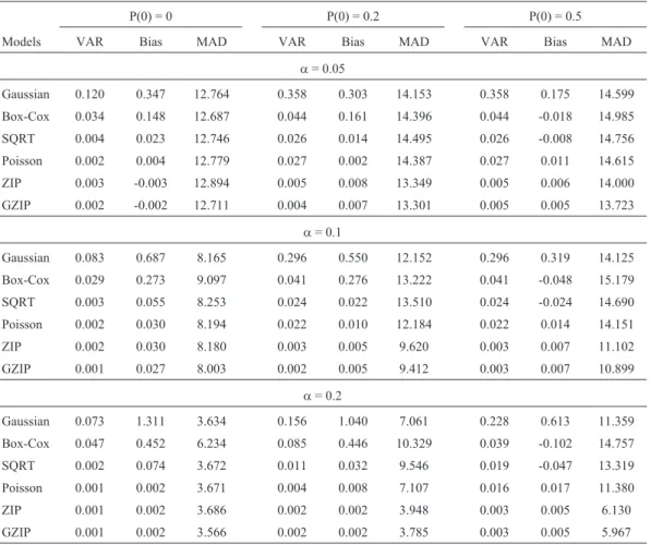
VAR, bias and MAD values (Table 3) indicate that, notwithstanding the scenario, the Gaussian model without transformation presented the worst results for VAR and bias, with transformations, more precisely by Box-Cox and SQRT, assuming a better stance, whereas with assumed normal SQRT transformation, the simplest and most used

for count data, performance was the best. As expected, the superiority of GLM approaches was eminently clear, espe-cially of ZIP and GZIP models, whose performances, al-though practically the same as Poisson when P(0) = 0, were far superior when P(0) = 0.2 and P(0) = 0.5.

As to MAD with a small additive QTL effect (a = 0.05), values were very similar for all the models. However, with an increase in QTL effect, ZIP and GZIP performances improved substantially compared to the other models. Generally speaking, all presented good values for MAD whena= 0.2, explainable by the higher the QTL ef-fect the higher the probability for detecting this QTL in the right position.

In summary, in view of the results (Tables 1, 2 and 3), it is possible to conclude that when there is moderate or ex-treme inflation of zeros, the best option is to adopt either the ZIP or GZIP models, since both are appropriate when reck-oning with the simultaneous occurrence of true zeros and zeros from Poisson distribution. Furthermore, with both, fi-nal results were very similar in all scenarios, since in the simulation studies under/over dispersion was disregarded, i.e.f= 1. Thus, as could be expected, GZIP can be charac-terized as a ZIP model. In any case, SQRT transformation

Table 2- The false positive discovery rate for each model in the different

percentage of zero inflation.

Model 1_{P(0) = 0 P(0) = 0.2 P(0) = 0.5}

Normal 18.7 15.9 17.9

Box-Cox 17.5 15.1 16.3

SQRT 18.6 15.9 16.2

Poisson 17.6 54.7 79.6

ZIP 17.5 17.3 17.6

GZIP 17.2 16.9 17.2

1_{P(.) stands for the probability of zeros in the simulated count data.}

Table 3- The variance, bias and mean of absolute distance for each model in the different simulated scenarios.

P(0) = 0 P(0) = 0.2 P(0) = 0.5

Models VAR Bias MAD VAR Bias MAD VAR Bias MAD

a= 0.05

Gaussian 0.120 0.347 12.764 0.358 0.303 14.153 0.358 0.175 14.599

Box-Cox 0.034 0.148 12.687 0.044 0.161 14.396 0.044 -0.018 14.985

SQRT 0.004 0.023 12.746 0.026 0.014 14.495 0.026 -0.008 14.756

Poisson 0.002 0.004 12.779 0.027 0.002 14.387 0.027 0.011 14.615

ZIP 0.003 -0.003 12.894 0.005 0.008 13.349 0.005 0.006 14.000

GZIP 0.002 -0.002 12.711 0.004 0.007 13.301 0.005 0.005 13.723

a= 0.1

Gaussian 0.083 0.687 8.165 0.296 0.550 12.152 0.296 0.319 14.125

Box-Cox 0.029 0.273 9.097 0.041 0.276 13.222 0.041 -0.048 15.179

SQRT 0.003 0.055 8.253 0.024 0.022 13.510 0.024 -0.024 14.690

Poisson 0.002 0.030 8.194 0.022 0.010 12.184 0.022 0.014 14.151

ZIP 0.002 0.030 8.180 0.003 0.005 9.620 0.003 0.007 11.102

GZIP 0.001 0.027 8.003 0.002 0.005 9.412 0.003 0.007 10.899

a= 0.2

Gaussian 0.073 1.311 3.634 0.156 1.040 7.061 0.228 0.613 11.359

Box-Cox 0.047 0.452 6.234 0.085 0.446 10.329 0.039 -0.102 14.757

SQRT 0.002 0.074 3.672 0.011 0.032 9.546 0.019 -0.047 13.319

Poisson 0.001 0.002 3.671 0.004 0.008 7.107 0.016 0.017 11.380

ZIP 0.001 0.002 3.686 0.002 0.002 3.948 0.003 0.005 6.130

proved to be an interesting and easy alternative to QTL de-tection in the presence of count data.

Motivating data set

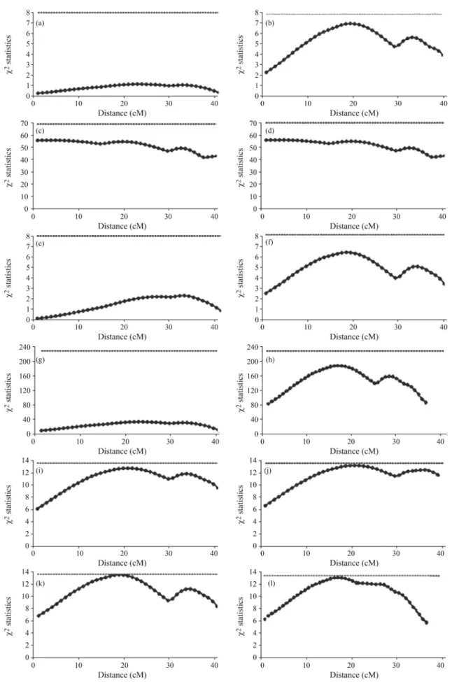
QTL profile-plots from five different models applied to first and second tick-count phenotypes in Holstein x Gyr cows, appear in Figure 1.

As there were less zeros in the data used for the first count than for the second, this could be used as a parameter for checking how the different models perform in the pres-ence of zero-counts and real zero-inflated counts. From the set of graphs related to the first count, it can be inferred that only simple (Figure 1 i) and generalized (Figure 1 k) ZIP models had come close to the 0.5% threshold, and that this was the only model that presented a “qtl” like curve. For the second set of graphs, except for that of Box-Cox transforma-tion, all the curves looked the same. As there apparently was a QTL around 21 cM, the ZIP models (Figure 1 j and l) showed that the curve had reached close to the 0.5% thresh-old. Through being compatible with those obtained with the simulated data set, the results revealed the superior perfor-mance of ZIP models when working with counting data in the high presence of zeros. Furthermore, the ZIP and GZIP models presented similar results in both tick counts, since in the GZIP fit, the estimatedfparameter came close to one, thereby indicating the absence of under/over dispersion.

In summary, we conclude that when working with nonormal distribution data, such as count data, prior de-scriptive analysis is always advisable. If working with zero-inflated data, it is recommended to use both simple and generalized ZIP models for data analysis. If working with data with zeros, but not zero inflated, either the Pois-son model or a data transformation approach, such as square-root transformation, can be employed. Square-root transformation can be used for Poisson distribution data, al-though in the case of uncertainty as to this being the case, a more general transformation, as Box-Cox, should be used instead.

Acknowledgments

This project was supported by CNPq and CAPES. We would also like to thank an anonymous reviewer for helpful suggestions and EMBRAPA-CNPGL.

References

Ascombe FJ (1948) The transformation of Poisson, binomial and negative-binomial data. Biometrika 35:246-254.

Baret PV, Knott SA and Visscher PM (1998) On the use of linear regression and maximum likelihood for QTL mapping in half-sib designs. Genet Res 72:149-158.

Box GEP and Cox DR (1964) An analysis of transformations. J R Stat Soc Series B Stat Methodol 26:211-252.

Chow NT and Steenhard D (2009) A flexible count data regres-sion model using SAS® PROC NLMIXED. In: SAS Global Forum: Statistics and Data Analysis 250:1-14.

Cui Y and Yang W (2009) Zero-inflated generalized Poisson re-gression mixture model for mapping quantitative trait loci underlying count trait with many zeros. J Theor Biol 256:276-285.

Cui Y, Kim DY and Zhu J (2006) On the generalized Poisson re-gression mixture model for mapping quantitative trait loci with count data. Genetics 174:2159-2172.

Erhardt V, Bogdan M and Czado C (2010) Locating multiple in-teracting quantitative trait loci with the zero-inflated gener-alized Poisson regression. Stat Appl Genet Mol Biol 9:e26. Frisch JE, O’Neill CJ and Kelly MJ (2000) Using genetics to

con-trol cattle parasites: The Rockhampton experience. Int J Parasitol 30:253-264.

Furlong J, Derez F, Matos LL and Balbi MV (1996) The effect of cattle tickBoophilus microplusinfestation on feed intake and milk yield of Holstein x Zebu crossbred cows. In: Pro-ceedings of the XV Panamerican Congress on Veterinary, Campo Grande, pp 340.

Gasparin G, Miyata M, Coutinho LL, Martinez ML, Teodoro RL, Machado MA, Silva MVGB, Sonstergard TS and Regitano LCA (2007) Mapping of quantitative trait loci controlling (Riphicephalus(Boophilus)microplus) resistance on bovine chromosomes 5, 7 and 14. Anim Genet 38:453-459. Haley CH, Knott SA and Elsen JM (1994) Mapping quantitative

trait loci in crosses between outbred lines using least squares. Genetics 136:1195-1207.

Lambert D (1992) Zero-inflated Poisson regression with an appli-cation to defects in manufacturing. Technometrics 34:1-14. Liu W and Cela J (2008) Count data models in SAS®. In: SAS

Global Forum: Statistics and Data Analysis 400:1-12. Martinez ML, Machado MA, Nascimento CS, Silva MVGB,

Teodoro RL, Furlong J, Prata MCA, Campos AL, Gui-marães MFM, Azevedo ALS,et al.(2006) Association of BoLA-DRB3.2 alleles with tick (Boophilus microplus) re-sistance in cattle. Genet Mol Res 5:513-524.

McCullagh P and Nelder JA (1989) Generalized Linear Models. 2nd edition. Chapman and Hall, Boca Raton, 402 pp. Nelder JA and Mead R (1965) A simplex method for function

minimization. Comput J 7:308-313.

Pérez-Enciso M and Misztal I (2004) Qxpak: A versatile mixed model application for genetical genomics and QTL analy-ses. Bioinformatics 20:2792-2798.

SAS Institute (2002) The SAS System for Windows. SAS Insti-tute, North Carolina, 502 pp.

Tilquin P, Coppieters W, Elsen JM, Lantier F, Moreno C and Baret PV (2001) Statistical power of QTL mapping methods applied to bacteria counts. Genet Res 78:303-316.

Wambura PN, Gwakis PS, Silayo RS and Rugaimukamu EA (1998) Breed-associated resistance to tick infestation in Bos indicus and their crosses withBos taurus. Veterinary Parasi-tology 77:63-70.

Yamamura K (1999) Transformation using (x+0.5) to stabilize the variance of populations. Journal Researches on Population Ecology 42:229-234.

Yang R, Yi N and Xu S (2006) Box-Cox transformation for QTL mapping. Genetica 128:133-143.

Associate Editor: Bertram Brenig