ISPRS International Journal of
Geo-Information
ISSN 2220-9964www.mdpi.com/journal/ijgi/ Article
Land Cover Mapping Analysis and Urban Growth Modelling
Using Remote Sensing Techniques in
Greater Cairo Region
—
Egypt
Yasmine Megahed *, Pedro Cabral, Joel Silvaand Mário Caetano
NOVA IMS Information Management School, Universidade Nova de Lisboa, Lisboa 1070-312, Portugal; E-mails: pcabral@novaims.unl.pt (P.C.); jsilva@novaims.unl.pt (J.S.);
mario@novaims.unl.pt (M.C.)
* Author to whom correspondence should be addressed; E-Mail: m2013313@novaims.unl.pt; Tel.: +2-356-00474.
Academic Editor: Wolfgang Kainz
Received: 17 August 2015 / Accepted: 27 August 2015 / Published: 14 September 2015
Keywords: urban growth modeling; cultural heritage; support vector machines; urban growth pattern
1. Introduction
Recent studies indicate that our world is undergoing the largest wave of urban growth in history [1]. One hundred years ago, two out of every ten people lived in an urban area, this number is expected to grow to reach six out of ten in 2030, and seven out of ten in 2050 [2]. The world’s urban residents began to increase significantly since the 1950s and it is expected to almost double, increasing from approximately 3.4 thousands of millionin 2009 to 6.4 thousands of millionin 2050 [2]. Consequently, this massive increase in urban population makes governments, policy makers, and civil society organizations face challenges in resources reallocation to overcome the problems that will arise in the future, to achieve a sustainable development of urban areas and to preserve cultural heritage from urban settlements being formed around areas of high legacy.
Models are simplifications of reality; they are theoretical abstractions that represent systems in such a way that essential features crucial to the theory and its application are identified and highlighted [3]. Land Use Land Cover Change (LULCC) models are tools to support the analysis of the causes and consequences of LULCC for a better understanding of the system functionality, and to support land-use planning and policy [4]. Models are useful for simplifying the complex suite of socioeconomic and biophysical forces that influence the rate and spatial pattern of LULCC and for estimating the impacts of changes [4].
Table 1. Different Land Use Land Cover Change (LULCC) models in recent studies.
Model Study Area Data Set Validation Technique Reference
MC-CA 1 Harbin, China Landsat TM 1989,
2007, ETM+2001
Kappa spatial correlation
statistic [5] [6]
LCM Asmara, Eritrea Landsat 1989,
2000, 2009
Kappa spatial correlation
statistic [7]
LTM-MC 2 SEWI
3, USA and
MRW 4, Michigan, USA
SEWI and MRW were digitized
manually.
ROC 5 [8] and PCM 6 [9,10] [11]
SLEUTH 7 Jimei, southeast coast of
Fujian Province, China
Landsat TM5 1992, 1997, 2002
and 2007
Lee-Sallee index [12]
1 MC-CA: Markov Chain-Cellular Automata; 2 LTM-MC: Land Transformation Model-Multiple
Classifications; 3 SEWI: South-Eastern Wisconsin; 4 MRW: Muskegon River Watershed; 5 ROC: Relative
Operating Characteristic; 6 PCM: Percent Correct Match; 7 SLEUTH: The name comes from an acronym for
There are four types of modeling approaches: machine learning, cellular sector-based economic, spatially disaggregated economic, and agent-based approaches [13]. Table 1 summarizes some model types in addition to the validation techniques that were applied in some LULCC studies.
Land Change Modeler (LCM) is an integrated software environment for analyzing and predicting LULCC, and for validating the results [14]. It is embedded in the IDRISI software [7], where only thematic raster images with the same land cover categories listed in the same sequential order can be input for LULCC analysis [15]. LCM evaluates land cover changes between two different times, calculates the changes, and displays the results with various graphs and maps. Then, it predicts future LULC maps on the basis of relative transition potential maps [15] relying upon Multi-Layer Perceptron (MLP) neural networks [16]. LCM was found to produce better prediction accuracy in short time scales, especially in the case of stable land covers rather than cases of rapid change [15]. When compared to models that predict LULCC based on supervised approaches (e.g., the Weights of Evidence method, where the weights can be selected and edited by a user), LCM generates more accurate overall change potential maps because neural network outputs are able to express the change of various land cover types more adequately than individual probabilities obtained through the Weights of Evidence method [16].
Different studies have previously been carried out for LULCC detection and modeling in the Greater Cairo Region (GCR). The ISODATA clustering procedure was used for image classification and the image differencing technique was applied to detect the LULCC between 1986 and 1999 [17]. The study indicated that urban areas increased from 344 km2 in 1986 to 460 km2 in 1999. Another study applied Maximum Likelihood classifier using ERDAS software for the LULCC detection in 1973 and 2006 [18]. The study applied post-classification comparison techniques for LUCC detection. Results showed that urban areas expanded from 224 km2 in 1973 to 558 km2 in 2006, with total agricultural cut-offs and
urbanized desert of 137 km2 and 187 km2, respectively. The Nearest Distance classifier was used to classify 1984, 2000 and 2008 images, and MC-CA integrated model with Multi Criteria Evaluation procedure was applied in a different study to select and evaluate the driving forces [19]. The model accuracy was 88%, indicating the validity of model parameters, and of the model to predict urban growth for 2038.
This study aims to detect the LULCC from 1984 to 2014, analyze the spatial and temporal growth patterns, and model the changes to predict the LULC in 2025 using LCM.
2. Study Area
The selected area for the study is the metropolitan area of Cairo, the political capital, and Qalyubia, in addition to parts of Giza City that belong to the Greater Cairo Region (GCR) (Figure 1). The study area is located at 30°02'N and 31°21'E, in the middle of the Delta Region, and covers an area of 8942 km2. Figure 1 shows three 5-km buffer zones around which the urban density will be calculated:
(1) The Great Giza Pyramids and the Sphinx area, representing the Pharaonic history.
(2) Al-Hussien Mosque, Khan Al-Khalily area, Al-Moez Street, and the Citadel, all in one area, representing an essential part of ancient Islamic Cairo.
The region has the highest population and population density among Egyptian governorates [20], and is considered one of the most populous regions worldwide [20]. The internal migration from Upper Egypt and the Delta began just after the Second World War, especially in the middle of 1950s due to the massive industrialization policy launched by President Nasser, which encouraged people to migrate, seeking better job opportunities and higher quality of education [21]. In 1947, the GCR hosted around three million people, representing 12.5% of the total Egyptian population at the time. This number kept growing to 13 million in 1996, representing 17.3% of the total Egyptian population [21], and, in 2006, it reached 16.1 million people [22]. Cairo City was the most populous among Egyptian cities in 2013, with almost nine million people, representing 10.7% of total population recorded in the same year [20]. Consequently, critical housing pressures began to appear in the GCR [21]. More than 75% of the population is living within only 30 km from the city center, moreover, the region’s urban development has been characterized by the rapid expansion of densely populated informal settlements, which reached 40% in 2009 [21].
Figure 1. Study area.
3. Data and Methods
3.1. Data
Three cloud free Landsat images for the years 1984, 2003, and 2014 were downloaded at no cost from EarthExplorer [26] (Table 2).
In addition to these datasets, ancillary data were also used: Google Earth maps [27], road networks [28], Digital elevation Model (DEM), and slope [26].
Table 2. Imageries attributes.
Acquisition
Date Sensor
Spatial
Resolution Path/Row Landsat
Number of Bands
Radiometric Resolution
15/03/2014 OLI-TIRS 30 m 176/39 Landsat 8 11 16 bits
07/07/2003 TM 30 m 176/39 Landsat 5 7 8 bits
02/07/1984 TM 30 m 176/39 Landsat 5 7 8 bits
OLI-TIRS: Operational Land Imager-Thermal Infrared Sensor; TM: Thematic Mapper
3.2. Methodology Overview
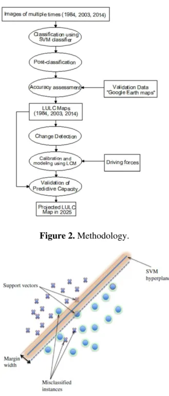
Figure 2 illustrates the flowchart of the methodology applied during the study. Multiple satellite scenes for the same study area, obtained at different time stamps (1984, 2003 and 2014), were classified to produce LULC maps. This classification was validated through an accuracy assessment process, which was performed with the aid of validation data or reference maps (e.g., Google Earth maps). The validation was followed by LULCC detection analysis to determine the amount of each class at time t1 that became another class by time t2. These transitions were recorded in a change matrixthat represented the input to the subsequent step; calibrating and modeling the transitions of interest. After the driving forces had been set, the transitions between 1984 and 2003 were modeled using LCM to produce a predicted map of 2014. This modeled map was compared to the LULC map of the same year, derived from satellite images, in order to validate the model. Once validated, the model was used with the same prediction time difference (11 years) using the 1984 and 2014 LULC maps to predict the LULC map for 2025.
3.3. LULC Maps Production and LULCC Detection
Figure 2. Methodology.
Figure 3. Linear support vector machine example.
other hand, for LULCC detection, there are two main groups of change detection techniques: binary change/no-change information, in which the output has only two possibilities; weather the pixel has changed, or not changed, within two specific time stamps [33]. The second approach yields a detailed “from-to” change trajectory, which results in a complete matrix with the exact amount of pixels turned from one class into another (e.g., post classification comparison) [33].
The problem while applying change or non-change detection techniques is the difficulty to precisely identify the thresholds [33]. Usually, methods used to select thresholds lead to external influences on the differences caused by atmospheric conditions, sun angles, soil moistures, and phonological differences, in addition to the threshold itself, is highly subjective and scene dependent, depending on the analyst’s familiarity with the study area [33]. The post classification comparison technique consists of an independent classification of each image, followed by a thematic overlay of the classifications, resulting in a complete “from–to” change matrix of the conversion between each class on the two dates [34]. The problem in this technique is the high effect of errors resulting from image classification on the change map. For example, two images classified with 80% accuracy might have only a 0.80 × 0.80 × 100 = 64% correct joint classification rate [34].
In the combination of both techniques, the change image is recoded into a binary mask consisting of areas that have changed between the two dates [35]. The change mask is then overlaid onto the second time stamp image and only those pixels that were detected as having changed are classified in the t2 imagery [35]. A traditional post-classification comparison can then be applied to yield complete “from-to” change information. This method may reduce change detection errors. Hence, in this study, a hybrid technique was applied, in which binary maps (areas of change/no-change) for both periods, 1984–2003 and 2003–2014, were produced using the combination of the Normalized Difference Vegetation Index (NDVI), Near Infrared (NIR), and Red differences technique, as it was found that the direct use of NDVI difference, by applying threshold values, failed to detect many urban settlements, while when combined with NIR difference and Red difference, it gave a better result of urban change [36]. Then, only areas of change were thematically overlaid to produce the change matrix in both periods; 1984–2003 and 2003–2014.
3.4. Spatial and Temporal Urban Growth Pattern Analysis
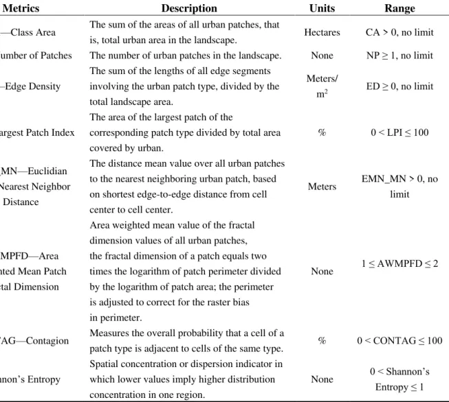
For urban sprawl analysis, FRAGSTATS software, version 4.2, was used to calculate spatial metrics for Urban classes over 30 years, from 1984 to 2014, based on the LULC maps of 1984, 2003, and 2014. The selected subset of matrices applied in the study is given in Table 3. They are the most commonly used and explored metrics in similar studies [37,38].
determines patches adjacency. The lower the CONTAG values are, the more heterogeneous the landscape becomes.
Table 3. Spatial metrics.
Metrics Description Units Range
CA—Class Area The sum of the areas of all urban patches, that
is, total urban area in the landscape. Hectares CA > 0, no limit NP—Number of Patches The number of urban patches in the landscape. None NP ≥ 1, no limit
ED—Edge Density
The sum of the lengths of all edge segments involving the urban patch type, divided by the total landscape area.
Meters/
m2 ED ≥ 0, no limit
LPI—Largest Patch Index
The area of the largest patch of the
corresponding patch type divided by total area covered by urban.
% 0 < LPI ≤ 100
ENN_MN—Euclidian Mean Nearest Neighbor
Distance
The distance mean value over all urban patches to the nearest neighboring urban patch, based on shortest edge-to-edge distance from cell center to cell center.
Meters EMN_MN > 0, no limit
AWMPFD—Area
Weighted Mean Patch Fractal Dimension
Area weighted mean value of the fractal dimension values of all urban patches, the fractal dimension of a patch equals two times the logarithm of patch perimeter divided by the logarithm of patch area; the perimeter is adjusted to correct for the raster bias in perimeter.
None 1 ≤ AWMPFD ≤ 2
CONTAG—Contagion Measures the overall probability that a cell of a
patch type is adjacent to cells of the same type. % 0 < CONTAG ≤ 100
Shannon’s Entropy
Spatial concentration or dispersion indicator in which lower values imply higher distribution concentration in one region.
None 0 < Shannon’s
Entropy ≤ 1
4. Model Implementation
LCM embedded in IDRISI 17.0 was used in this study to predict the LULC map in 2025 using the following procedure: change analysis, transition potential modeling and driving forces determination, change prediction, and model validation. In the change analysis step, the changes were assessed between 1984 and 2003. These changes represent the transitions from one class to another, which are important in order to identify the dominant transitions to urban and target them for modeling [39].
4.1. Transition Potential Modeling and Driving Forces Determination
areas in 1984 were set as predictor variables. They were chosen based on recent similar studies [19] in which they were found to highly affect urban sprawl, and were based on the LULCC between 1984 and 2003, where new urban settlements were noticed to occur near the built-up areas and the road network. Distance to urban areas in 1984 was defined as a dynamic factor and was recalculated over the prediction period (11 years, from 2003 to 2014), as an urban area expands, consequently, distance to urban areas in 1984 will vary over time. Likewise, the distance to roads in 2003 should have been considered as a dynamic factor, as new roads are assumed to be built between 2003 and 2014. This could be applied in case the roads were obtained in 2003, but as long as the roads were in 2014, this driving force was set as static.
LCM provides an optional quick test of the potential explanatory power of each driving force represented by Cramer’s V. It is a correlation coefficient that ranges from 0.0, indicating no correlation (discarded variable), to 1.0, indicating perfect correlation (excellent potential variable) [14]. Although it does not guarantee a strong performance because it cannot account for the mathematical requirements and the complexity of the relationship [40], it acts as a guide to determine whether the driving force is worth being considered or not [14]. Multi-Layer Perceptron (MLP) neural network is a feedforward neural network in which data flows in one direction from an input layer to an output layer through hidden layer(s) in between [41]. The computing elements (nodes) are grouped into layers and each node receives an input signal from other nodes after processing the signals locally through a transfer function, it outputs a transformed signal to other nodes or final result [42]. Each signal feeding into a node in a subsequent layer has the original input multiplied by a weight with a threshold added and then is passed through an activation function that may be linear or non-linear (hidden units) [42]. The weights have to be determined in the training process before the network can be used for prediction purposes, using part of the data, aiming at changing the weights so as to minimize the error between the observed and the predicted outcomes [42]. A MLP neural network allows for modeling more than one transition at a time [14], hence, it was applied in this study.
4.2. Change Prediction
In this step, LCM uses the change rates calculated from the first step, as well as the transition potential maps produced from the second step, to predict a future scenario for 2014. This step is responsible for determining the quantity of change to urban areas in each transition in 2014 using MC analysis [14]. There are two basic types of predictions: hard and soft predictions [14]. Hard prediction yields a projected map of 2014, where each pixel is assigned one land cover class; the class that it is most likely to become. Soft prediction, however, is different, as it produces a vulnerability map in which each pixel is assigned a value from 0.0 to 1.0, indicating the probability of the pixel to become urban in 2014 [14].
4.3. Model Validation
(1) Hits: Model predicted change and it occurred in reality.
(2) False alarms: Model predicted change to urban areas while it persisted in reality. (3) Misses: Model predicted persistence and it became urban in reality.
(4) Null success: Model did not predict change and it did not occur in reality.
False alarms and misses represent the errors that resulted from the model as a disagreement between the simulated map and the reference map, while hits and null success represent the model correctness [8]. To determine the overall agreement between observed and predicted maps, we calculated the Figure of Merit (FOM), which is a ratio between hits and the summation of hits, misses, and false alarms. It ranges from 0%, meaning no overlap between the observed and predicted change, to 100%, meaning a perfect overlap between the observed and predicted change [43]. On the other hand, the statistical approach examines the agreement between a pair of maps that show any categorical variable, which can have any number of categories [8]. The map of reality acted as the reference map, while the simulated map was the comparison map. In this study, Kappa variations were applied: Kno and Klocalion, where Kno is the
overall accuracy of the simulation run and Klocation indicates the level of agreement of location [44]. We
eliminated the usage of Kstandard (the proportion assigned correctly versus the proportion that is correct
by chance [45])in this study, as it was not found to be helpful to interpret, while Klocalion can be somewhat
helpful [46]. Once the model predictive power was assessed, it was used to predict 2025’s LULC map, with the same driving forces, modeling the changes between 1984 and 2014’s LULC maps.
5. Results and Discussion
5.1. LULC Maps Production and LULCC detection
The accuracy assessment resulted in an overall accuracy of 96%, 97.3%, and 96.3%, for 1984, 2003, and 2014’s LULC maps (Figure 4), respectively. The most significant changes in both periods (1984–2003 and 2003–2014) are the transitions from vegetation and desert to urban areas. Over 19 years, from 1984 to 2003, vegetation lost 13% to urban, representing 19,179 hectares, and almost the same percentage (12%) within only 11 years, from 2003 to 2014, representing an amount of 16,486 hectares. This indicates the massive leveling of agricultural lands in the GCR for urbanization purposes, especially during the last decade, because of the absence and/or the inactivation of farmland protection laws. Additionally, 3% of desert areas became urban between 1984 and 2003, which is equivalent to 21,417 hectares. This percentage increased to 5% between 2003 and 2014, representing 31,045 hectares, resulting from the application of desert reconstruction strategies to build new communities outside the Nile Valley.
5.2. Spatial and Temporal Urban Growth Pattern Analysis
By contrast, ENN_MN dipped from 1984 to 2014, meaning that the space between urban neighbors is shrinking over time as a result of higher urbanization density.
AWMPFD climbed from 1.31 to 1.45 between 1984 and 2003, while, later, it increased steadily to reach 1.46 in 2014. This means that the level of complexity and fragmentation is increasing for the landscape patches. The drop in CONTAG values between 1984 and 2014 may have resulted from higher fragmentation due to more individual urban units. Finally, Shannon’s Entropy values have gradually increased over the study period because of the more-dispersed distribution taking place in the GCR.
LULC map—1984 LULC map—2003 LULC map—2014
Figure 4. LULC maps.
Figure 5. Temporal urban growth signatures of spatial metrics (Class Area, Number of Patches, Edge Density, Largest Patch Index, Euclidian Mean Nearest Neighbor Distance, Area Weighted Mean Patch Fractal Dimension, Contagion, and Shannon’s Entropy).
5.3. Model Implementation
5.3.1. Transition Potential Modeling and Driving Forces Determination
The LULCC results indicated two significant changes to urban areas: from vegetation and from desert, consequently, both were the model’s major transitions. Both transitions to urban areas had the same driving forces, depending on the visual examination of the urban spatial trend, which indicated that the selected predictor variables affect both of them. Table 4 illustrates the potential explanatory power of each driving force, represented by Cramer’s V. The variables that have a Cramer’s V of about 0.15 or higher are useful, while those with values of 0.4 or higher are good [14]. Thus, the selected factors were found to be relevant and worth consideration.
After the selection of the predictor variables, both transitions were modeled in one transition sub-model, as they had the same driving forces, with the aim of producing the transition maps.
Table 4.Cramer’s V values of the selected driving forces of change.
Driving Force Cramer’s V
DEM 0.55
Slope 0.49
Distance to roads in 2014 0.25
5.3.2. Model Validation
The visual validation of the simulated change in 2014 resulted in a map of correctness and error, given in Figure 6. The map consists of 1.31% hits, 89.73% null successes, 2.30% false alarms, and 6.66% misses. The simulated change is 3.61% of the landscape, less than the observed change, which is 7.97% of the landscape, and this is why the error occurred. In this case, the FOM is 12.76%, which is a low performance, emphasizing the importance of considering further predictive variables, as is obvious from the results that the applied driving forces are not enough to model this large area of study. Moreover, Figure 6 shows the distribution of the misses, which are highly concentrated in the second transition, from desert to urban, meaning that modeling the urbanization in the desert parts should be done using a set of driving forces different from the set used to model the first transition, from vegetation to urban. Obtaining data about Cairo is always a problematic issue due to the lack of available data and the change of administrative boundaries of the governorates, which yield some areas with no data. The problem is especially highlighted when dealing with a large region like the GCR, where three main cities are included, thus, we were unable to include extra variables in this study (e.g., distance to industrial areas and commercial centers). However, the results are still higher than some recent studies where FOM was 10.4 and 2.9% [39,43]. Although visual examination is the quickest way to reveal spatial patterns, which statistical methods may fail to detect, it is subjective and can be misleading, therefore, the statistical approach is essential [8].
On the other hand, Kappa variations that compared the projected LULC in 2014 with the actual LULC map in 2014 resulted in Kno and Klocalion of 92.88% and 94.24%, respectively. The interpretation of these
high values is that the majority of the study area experienced no change, as, even with the new urban communities that were constructed in the desert areas during the last 30 years (from 1984 to 2014), the desert forms the major land cover that was not subjected to high urbanization during this period. Because of this, it was essential to perform the visual validation throughout the FOM test, as, although Kappa coefficients obtained in this study are above 90%, better than what was obtained in similar studies [47,48], comparing both results reveals the fact that the correct localization of the projected LULCC in areas of change is more pronounced than that in areas of no change. However, Kappa statistic results are more promising than visual validation.
5.3.3. LULC Map Prediction for 2025
The changes between 1984 and 2014 were modeled using the real LULC maps in order to predict the LULC map of 2025 with the same prediction period (11 years). Fourteen percent of the vegetation and 4% of the desert in 2014 are expected to transition to urban areas in 2025, which is equivalent to 16,512 and 24,687 hectares, respectively. Figure 7 shows the urban growth in the GCR in 1984, 2003, 2014, and the estimated urban settlements in 2025. Urban expansion has boomed over 30 years, from 1984 to 2014, and the modeling results confirm that it will be increasing to 2025. The urban areas were 41,488, 95,793 and 154,861 hectares in 1984, 2003, and 2014, representing 4.64%, 10.71%, and 17.32% of the total area of the GCR, respectively. In 2025, according to the model estimations, the urban areas in the GCR will expand to 196,047 hectares, which is about 21.93% of the region. This vast, unplanned growth is a serious threat towards the ecological system, as there is an obvious tendency of a continuous agricultural loss with increasing rates: 13%, 12%, and 14% within 19, 11, and 11 years between 1984–2003, 2003–2014, and 2014–2025, respectively. This implies a current and upcoming threat to the cultural heritage of the GCR, especially with the increasing population in the Egyptian capital.
5.3.4. The Future Effect of Urban Sprawl on the Cultural Heritage
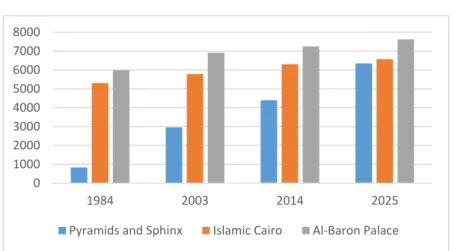
Figure 7. Urban growth in the GCR.
Figure 8. Total area of urban patches within 5-km buffer around cultural monuments (hectares).
6. Conclusions
This study was performed to detect and analyze the urban growth in the GCR over a period of 30 years, from 1984 to 2014, and to model the changes to estimate the urban area in 2025. Three Landsat scenes obtained in 1984, 2003, and 2014 were classified using SVM classifier. LULCC detection was determined using a high-level land-cover mapping-technique, which combines binary maps of change/no-change information with post-comparison approach. From 1984 to 2003, 13% of the vegetation was lost to urban areas, and 12% was lost between 2003 and 2014, representing 19,179 and 16,486 hectares, respectively. While 3% of desert areas became urban between 1984 and 2003,
0 1000 2000 3000 4000 5000 6000 7000 8000
1984 2003 2014 2025
it increased to 5% between 2003 and 2014, which are equivalent to 21,417 and 31,045 hectares, respectively. The absence of low activation against agricultural land leveling and the application of desert reconstruction strategies, to build new communities outside the Nile Valley, are the main reasons for such massive urbanization.
Eight metrics were computed using FRAGSTATS to analyze the spatial and temporal urban growth, all emphasise the more dense urbanization taking place in the GCR, as well as the dispersed and fragmented landscape as a result of individual urban establishment. The transitions from vegetation and desert to urban were modeled using LCM, with the driving forces: DEM, slope, distance to road network, and distance to existing urban areas. These factors were considered in similar studies and proved to dominate the urbanization for future scenarios. Areas with a high slope clearly represent less of a tendency to become urban [19], and areas of low elevation are most likely to become urban. From the visual inspection of the LULC maps, it was clear that new built-ups tend to be near the existing urban areas and road networks, to make use of the available infrastructures, services, and facilities.
To validate the model, the simulated 2014 map was examined against 2014’s real LULC map, applying both visual and statistical approaches, via FOM and Kappa statistics, respectively. Kappa coefficients (Kno and Klocalion) were above 90% because the majority of the study area experienced no
change, however they are more promising than the FOM, which resulted in 12.76%. The FOM results highlighted the problem of insufficient predicting variables and modeling both transitions (from vegetation and desert to urban) using the same driving forces, as the majority of the misses occurred in the new built-ups in the desert areas. The projected 2025 LULC map estimates an urban transition of 14% from vegetation and 4% from desert, between 2014 and 2025, which are equivalent to 16,512 and 24,687 hectares, respectively.
On the other hand, the areas of urban patches were calculated over time (from 1984 to 2025) in a 5-km buffer around three main historical places in the GCR: the Great Pyramids, Islamic Cairo, and Al-Baron Palace. The results showed similar gradual patterns of urban expansion around Islamic Cairo and Al-Baron Palace, as they both have been surrounded by dense urban settlements. This trend is estimated to continue increasing in 2025 around Al-Baron Palace, whereas no further significant urban development is expected to occur within a 5-km ring around the Islamic Cairo area, as it is already full of urban, showing no promising vacancies for further settlements. However, the Pyramids’ area showed a booming urbanization since the urban density in 2014 was five times what it had been in 1984, moreover, this trend is estimated to increase in 2025 to be almost equal to the Islamic Cairo records. These results imply that the Egyptian cultural heritage will be surrounded by urban areas, especially around the Pyramids’ area, indicating a gradual loss of value and of its unique appearance. If this trend continues, protection policies have to be undertaken to preserve the cultural heritage and the agricultural fields that will be negatively affected.
Acknowledgments
Author Contributions
Yasmine Megahed performed all the GIS analyses, processed the data and the model, wrote the paper, and delivered the manuscript. Pedro Cabral contributed to the conception of the research idea, reviewed FRAGSTATS and LCM results, edited and reviewed the overall design. Joel Silva helped in image classification using SVM, as well as image pre- and post-processing. He reviewed the LULC maps and the manuscript. Mário Caetano suggested the hybrid technique that was followed in LULCC detection and reviewed the results related to this part. All authors read and approved the final manuscript.
Conflicts of Interest
The authors declare no conflict of interest.
References
1. United Nations Fund for Population Activities. Urbanization: A Majority in Cities. Available online: http://www.unfpa.org/pds/urbanization.htm (accessed on 23 July 2014).
2. World Health Organization. Urbanization: Urban Population Growth. Available online: http://www.who.int/gho/urban_health/situation_trends/urban_population_growth_text/en/ (accessed on 23 July 2014).
3. Batty, M. Urban modeling. In International Encyclopedia of Human Geography; Elsevier: Oxford, UK, 2009; pp. 51–58.
4. Verburg, P.H.; Schot, P.P.; Dijst, M.J.; Veldkamp, A. Land use change modelling: Current practice and research priorities. GeoJournal 2004, 61, 309–324.
5. Mitsova, D.; Shuster, W.; Wang, X. A cellular automata model of land cover change to integrate urban growth with open space conservation. Landsc. Urban Plan. 2011, 99, 141–153.
6. Gong, W.; Li, Y.; Fan, W.; Stott, P. Analysis and simulation of land use spatial pattern in Harbin prefecture based on trajectories and cellular automata—Markov modelling. Int. J. Appl. Earth Obs. Geoinf. 2015, 34, 207–216.
7. Tewolde, M.G.; Cabral, P. Urban sprawl analysis and modelling in Asmara, Eritrea. Remote Sens.
2011, 3, 2148–2165.
8. Pontius, R.G., Jr.; Chen, H. Land Change Modeling with GEOMOD. Available online: http://planet.botany.uwc.ac.za/nisl/computing/IDRISI_andes/Documentation/Land%20Change%2 0Modeling%20with%20GEOMOD.pdf (accessed on 15 January 2015)
9. Tayyebi, A.; Pijanowski, B.C.; Pekin, B. Two rule-based urban growth boundary models applied to the Tehran Metropolitan Area, Iran. Appl. Geogr. 2011, 31, 908–918.
10. Tayyebi, A.; Pekin, B.K.; Pijanowski, B.C.; Plourde, J.D.; Doucette, J.S.; Braun, D. Hierarchical modeling of urban growth across the conterminous USA: Developing meso-scale quantity drivers for the Land Transformation Model. J. Land Use Sci. 2013, 8, 422–442.
12. Hua, L.; Tang, L. ; Cui, S.; Yin, K. Simulating urban growth using the Sleuth Model in a coastal peri-urban district in China. Sustainability 2014, 6, 3899–3914.
13. Brown, D.G.; Walker, R.; Manson, S.; Seto, K. Modeling land-use and land-cover change. In Land Change Science; Springer: Houten, The Netherlands, 2004; pp. 395–409.
14. Eastman, J.R. IDRISI Selva Tutorial. Available online: http://uhulag.mendelu.cz/files/pagesdata/ eng/gis/idrisi_selva_tutorial.pdf (accessed on 15 December 2014).
15. Roy, H.G.; Dennis, M.F.; Emsellem, K. Predicting land cover change in a Mediterranean catchment at different time scales. In Computational Science and Its Applications—ICCSA 2014, Springer International Publishing: Basel, Switzerland, 2014; pp. 315–330.
16. Vega, P.A.; Mas, J.F.; Zielinska, A.L. Comparing two approaches to land use/cover change modelling and their implications for the assessment of biodiversity loss in a deciduous tropical forest. Environ. Model. Softw 2012, 29, 11–23.
17. Yin, Z.Y.; Stewart, D.J.; Bullard, S.; Maclachlan, J.T. Changes in urban built-up surface and population distribution patterns during 1986–1999: A case study of Cairo, Egypt. Comput. Environ. Urban Syst. 2005, 29, 595–616.
18. Mohamed, E. Analysis of urban growth at Cairo, Egypt using remote sensing and GIS. Nat. Sci.
2012, 4, doi:10.4236/ns.2012.46049.
19. de Noronha Vaz, E.; Caetano, M.; Nijkamp, P. Trapped between antiquity and urbanism—A multi-criteria assessment model of the Greater Cairo Metropolitan Area. J. Land Use Sci. 2011, 6, 283–299.
20. State Information Service. Egypt Gateway. Available online: http://www.sis.gov.eg/En/Default.aspx (accessed on 26 September 2014).
21. Howeidy, A.; Shehayeb, D.K.; Göll, E.; Halim, K.M.A.; Séjourné, M.; Gado, M.; Piffero, E.; Haase-Hindenberg, G.; Löffler, G.; Stryjak, J.; et al. Cairo’s Informal Areas: Between Urban Challenges and Hidden Potentials—Facts, Voices and Visions; Kipper, R., Fischer, M., Eds.; GTZ Egypt: Cairo, Egypt, 2009.
22. Central Agency for Public Mobilization and Statistics. Available online: http://www.capmas. gov.eg/Default.aspx?lang=2 (Accessed 20 September 2014).
23. Huang, W.; Liu, H.; Luan, Q.; Jiang, Q.; Liu, J.; Liu, H. Detection and prediction of land use change in Beijing based on remote sensing and GIS. Int. Arch. Photogramm. Remote Sens. Spat. Inf. Sci.
2008, 37, 75–82.
24. Epstein, J.; Payne, K.; Kramer, E. Techniques for mapping suburban sprawl. Photogr. Eng. Remote Sens. 2002, 63, 913–918.
25. Möller, M.S. Remote Sensing for the Monitoring of Urban Growth Patterns. Available online: http://www.isprs.org/proceedings/XXXVI/8-W27/moeller.pdf (accessed on 10 September 2014). 26. EarthExplorer. Available online: http://earthexplorer.usgs.gov/ (accessed on 20 September 2014). 27. Google Maps. Available online: https://maps.google.com/ (accessed on 20 November 2014). 28. OpenStreetMaps (OSM). Available online: https://www.openstreetmap.org/ (accessed on 20
November 2014).
30. Mountrakis, G.; Jungho, I., Ogole, C. Support vector machines in remote sensing: A review. ISPRS J. Photogramm. Remote Sens. 2011, 66, 247–259.
31. Pal, M.; Mather, P.M. Support vector machines for classification in remote sensing. Int. J. Remote Sens. 2005, 26, 1007–1011.
32. Singh, S.K.; Srivastava, P.K.; Gupta, M.; Thakur, J.K., Mukherjee, S. Appraisal of land use/land cover of mangrove forest ecosystem using support vector machine. Environ. Earth Sci. 2014, 71, 2245–2255.
33. Weng, Q. Remote sensing image classification. In Advances in Environmental Remote Sensing: Sensors, Algorithms, and Applications; CRC Press: Boca Raton, FL, USA, 2011.
34. Singh, A. Review article digital change detection techniques using remotely-sensed data. Int. J. Remote Sens. 1989, 10, 989–1003.
35. Mas, J.F. Monitoring land-cover changes: A comparison of change detection techniques. Int. J. Remote Sens. 1999, 20, 139–152.
36. Veettil, B.K. A Comparative study of urban change detection techniques using high spatial resolution images. In Proceedings of the 4th GEOBIA, Rio de Janeiro, SP, Brazil, 7–9 May 2012. 37. Araya, Y.H.; Cabral, P. Analysis and modeling of urban land cover change in Setúbal and Sesimbra,
Portugal. Remote Sens. 2010, 2, 1549–1563.
38. Herold, M.; Goldstein, N.C.; Clarke, K.C. The Spatiotemporal form of urban growth: Measurement, analysis and modeling. Remote Sens. Environ. 2003, 86, 286–302.
39. Olmedo, M.T. C.; Paegelow, M.; Mas, J.F. Interest in intermediate soft-classified maps in land change model validation: Suitability versus transition potential. Int. J. Geogr. Inf. Sci. 2013, 27, 2343–2361.
40. Khoi, D.D., Murayama, Y. Forecasting areas vulnerable to forest conversion in the Tam Dao National Park Region, Vietnam. Remote Sens. 2010, 2, 1249–1272.
41. Nazzal, J.M.; El-Emary, I.M.; Najim, S.A. Multilayer perceptron neural network (MLPs) for analyzing the properties of Jordan oil shale. World Appl. Sci. J. 2008, 5, 546–552.
42. Sibanda, W.; Pretorius, P. Novel application of Multi-Layer Perceptrons (MLP) neural networks to model HIV in South Africa using Seroprevalence data from antenatal clinics. Int. J. Comput. Appl.
2011, 35, 26–31.
43. Rodríguez, N.E.; Armenteras-Pascual, D.; Alumbreros, J.R. Land use and land cover change in the Colombian Andes: Dynamics and future scenarios. J. Land Use Sci. 2013, 8, 154–174.
44. Nadoushan, M.A.; Soffianian, A.; Alebrahim, A. Predicting urban expansion in Arak Metropolitan Area using two land change models. World Appl. Sci. J. 2012, 18, 1124–1132.
45. Kim, I.; Jeong, G.Y.; Park, S.; Tenhunen, J. Predicted land use change in the Soyang River Basin, South Korea. In Proceedings of 2011 TERRECO Science Conference, Garmisch-Partenkirchen, Germany, 2–7 October 2011.
46. Pontius, J.; Robert, G., Marco, M. Death to Kappa: Birth of quantity disagreement and allocation disagreement for accuracy assessment. Int. J. Remote Sens. 2011, 32, 4407–4429.
48. Subedi, P.; Subedi, K.; Thapa, B. Application of a hybrid cellular automaton-markov (CA-Markov) model in land-use change prediction: A case study of Saddle Creek Drainage Basin, Florida. Appl. Ecol. Environ. Sci. 2013, 1, 126–132.