Control of phytoplankton production by physical forcing in a strongly tidal, well-mixed estuary

www.biogeosciences.net/bg/2/205/ SRef-ID: 1726-4189/bg/2005-2-205 European Geosciences Union

Biogeosciences

Control of phytoplankton production by physical forcing in a

strongly tidal, well-mixed estuary

X. Desmit1, J. P. Vanderborght1, P. Regnier2, and R. Wollast1, †

1_{Laboratory of Chemical Oceanography and Water Geochemistry and Department of Water Pollution Control, Universit´e}

Libre de Bruxelles, Boulevard du Triomphe (CP208), 1050 Brussels, Belgium

2_{Biogeochemical System Dynamics, Department of Geochemistry, Utrecht University, PO Box 80.021, 3508 TA Utrecht, The}

Netherlands

†_{Deceased on 28 July 2004}

Received: 29 December 2004 – Published in Biogeosciences Discussions: 14 January 2005 Revised: 4 July 2005 – Accepted: 18 July 2005 – Published: 4 August 2005

Abstract. A zero-dimensional model for phytoplanktonic production in turbid, macro-tidal, well-mixed estuaries is proposed. It is based on the description of light-dependent algal growth, phytoplankton respiration and mortality. The model is forced by simple time-functions for solar irradiance, water depth and light penetration. The extinction coefficient is directly related to the dynamics of suspended particulate matter. Model results show that the description of phyto-plankton growth must operate at a time resolution sufficiently high to describe the interference between solarly and tidally driven physical forcing functions. They also demonstrate that in shallow to moderately deep systems, simulations us-ing averaged, instead of time-varyus-ing, forcus-ing functions lead to significant errors in the estimation of phytoplankton pro-ductivity. The highest errors are observed when the temporal pattern of light penetration, linked to the tidal cycle of solids settling and resuspension, is neglected. The model has also been applied using realistic forcing functions typical of two locations in the Scheldt estuary. Model results are consistent with the typical phytoplankton decay observed along the lon-gitudinal, seaward axis in the tidal river and oligohaline part of this estuary.

1 Introduction

Estuaries are often subject to high nutrient loads, which may lead to local eutrophication of the water masses. In tur-bid estuaries, however, phytoplankton respiration can exceed biomass production because of the low light penetration into the water column. This results in a negative depth-integrated Correspondence to:X. Desmit

(xdesmit@ulb.ac.be)

net primary production (NPP) (Grobbelaar, 1985; Reid et al., 1990; Cole et al., 1992; Heip et al., 1995). Neverthe-less, high phytoplankton biomass concentrations are com-monly observed in these environments (Kromkamp et al., 1995; Kromkamp and Peene, 1995; Heip et al., 1995 and references therein). Various authors have used the “critical mixing depth” approach introduced by Sverdrup (1953) to explain this apparent contradiction (Cole et al., 1992; Fichez et al., 1992; Irigoien and Castel, 1997). It is indeed well established that net phytoplankton production is determined by the ratio between critical and mixing depths, the for-mer being defined as the depth at which vertically integrated photosynthesis equals vertically integrated respiration (Sver-drup, 1953; Grobbelaar, 1985; Cloern, 1987; Falkowski and Raven, 1997). In this production-loss balance, the first term (vertically integrated photosynthesis) not only depends on bi-ological parameters: it is strongly linked to the light avail-ability within the water column, which is itself controlled by physical forcing mechanisms. This control is particularly critical in turbid environments such as estuaries and coastal waters, which are often under the influence of significant par-ticulate terrigeneous fluxes (Postma, 1980).

pertains to scientific disciplines that have largely evolved independently. Many authors have studied the correlation between phytoplankton production and turbidity, using the composite parameterBZE: biomassB, euphotic depth Z and solar irradianceE (Cole and Cloern, 1984; Harding et al., 1986; Cole and Cloern, 1987; Keller, 1988; Cole, 1989; Boyer et al., 1993; MacIntyre and Cullen, 1996). This em-pirical model may explain a large part of the variability of phytoplankton production in many estuaries, especially at the seasonal scale. However, the BZE model does not rely upon a physiological basis. In particular, it lacks any description of the phytoplankton response to light intensity (MacIntyre and Cullen, 1996). More critically, it does not link the value of the euphotic depth to the short-term suspended particulate matter (SPM) dynamics.

More recently, some authors have demonstrated how the short-term variation of various physical and biological pro-cesses influence the estuarine phytoplankton production. In particular, Lucas et al. (1999a, b) and Lucas and Cloern (2002) have shown that the interaction between water depth and bottom grazing may partially explain the occurrence of phytoplankton blooms in the South San Francisco Bay (SSFB). In their discussion over physical-biological phasing, they conclude that “other mechanisms of hourly scale vari-ability (. . . ) – such as short-term variations in water column irradiance caused by tidally driven sediment resuspension and diel light cycle - could contribute additional hourly scale physical-biological phasing processes” (Lucas et al., 1999b). Also in SSFB, May et al. (2003) have studied the short term variation of turbidity linked to wind-driven sediment resuspension. In this particular case, the tidal forcing is in-sufficient to resuspend sediments. This mechanism, and its coupling with the diel light cycle, have therefore not been considered in their work.

In this paper, the focus is on nutrient-rich, well-mixed tidal estuaries, where phytoplankton growth is not limited by nu-trient availability, but where light is the crucial control fac-tor. In such systems, it is expected that the underwater light field be not only determined by the incident solar irradiance, but also by the tidal influence on hydrodynamics and sedi-ment transport (Wofsy, 1983). Estimating the combined ef-fect of these forcing processes on the spatial and temporal evolution of phytoplankton production is clearly not a trivial question. The scope of this study is to assess the importance of the temporal, short-term variability of physical forcings and their interactions. More specifically, we investigate how short-term, tidally driven physical forcings interfere with the incident sunlight energy to sustain phytoplankton production in these environments. The impact of chlorophylla resus-pension on the estimate of depth-integrated phytoplankton production is also discussed. Note that our focus is not on the role of the spatial (horizontal) variability of the phyto-plankton production along the bathymetric gradient in an es-tuarine cross-section: this aspect has already been explored by a number of authors in the case of estuarine environments

where extended shallow zones interact with deeper channels (Lucas et al., 1999a, b). The paper is structured as follows: first, a simple model of phytoplankton biomass for strongly tidal, well-mixed estuaries is presented. It is then applied to an idealized case using simple periodic forcing functions, in order to highlight the main features of the systems response. Finally, more complex forcing conditions are applied, taking the Scheldt estuary (Belgium, The Netherlands) as an exam-ple of a typical well-mixed, turbid system displaying a high dynamical suspended matter behavior (Fettweis et al., 1998).

2 Model description

The main purpose of this study is to investigate whether or not a positive algal growth can be sustained in a turbid, well-mixed estuary, where the mixing depth is always larger than the euphotic depth (i.e. where benthic photosynthesis does not occur). To answer this question, we hypothesize that the turbidity, and hence the light regime, is essentially controlled by local hydrodynamic conditions. In other words, the dy-namics of suspended particulate matter (SPM) results mainly from local exchange fluxes with the bed through the pro-cesses of resuspension and deposition. This implies that the instantaneous current velocity is the key factor for turbidity. In addition, our focus is on the effect of local physical con-ditions on the sustainability of local algal growth; it is not on the effect of advective or diffusive transport on phytoplank-ton concentration along the longitudinal gradient. As a result, a simple box approach is adequate for our purpose. The use of more complex transport-reaction models of the estuarine continuum (e.g. Regnier and Steefel, 1999; Vanderborght et al., 2002) is therefore not required. Our modeling approach is very similar to the one of Lucas and Cloern (2002) who also neglected horizontal variability and transport processes in a zero-dimensional model of the phytoplankton dynamics in an idealized water column submitted to the semidiurnal tide.

2.1 Governing equations for a well-mixed reservoir of os-cillating depth

Consider a well-mixed reservoir of unit surface area, whose volume is changing with time due to the tidal variation of the depth zmax(t )(Fig. 1). The volume change is caused

Table 1.Notation, value and units of the parameters used in the model.

Parameters Notation Value Units

Specific photosynthetic efficiency αB 0.05 (µgC.µgChl−1.h−1). (µmol quanta.m−2.s−1)−1 Specific light-saturation rate of photosynthesis P_maxB 13 µgC.µgChl−1.h−1

Rate constant for maintenance respiration ρm 0.002 h−1

Growth respiration factor ρg 0.3 none

Excretion factor ε 0.03 none

Rate constant for mortality m 0.002 h−1

Carbon: Chlorophyllaratio θ 50 gC.gChl−1

Solar constant Ksol 1367 W.m−2

Sediment transport coefficient (location 1) X 2000 mg.L−1.m3.s−5

Sediment transport coefficient (location 2) X 6000 mg.L−1.m3.s−5

Wash load (location 1) Y 40 mg.L−1

Wash load (location 2) Y 25 mg.L−1

result, the governing equation must be written in terms of the total biomassBtotwithin the reservoir:

dBtot

dt = Q(t ) B(t ) + 1 θ

Z zmax(t )

0

r(z, t ) dz , (1) wherer(z, t )is the rate of phytoplankton biomass production at any timetand depthzwithin the reservoir. The conversion factorθ(chlorophyllato carbon ratio) is introduced in this equation for unit consistency. The algal biomassBis related toBtotaccording to:

B= Bt ot zmax

, (2)

while the rate of change of the water depth is given by: dzmax

dt =Q(t ) . (3)

2.2 Rate of algal growth

The raterof phytoplankton biomass production is given by:

r=NPP−Excr−Mor, (4)

where NPP is the net primary production of phytoplankton, Excr is the excretion rate (release of dissolved organic car-bon) and Mor is the mortality rate of the algal cells. The net primary production is defined as:

NPP=GPP−Resp, (5)

where GPP is the gross primary production of phytoplankton and Resp is the algal respiration rate. All rates are usually expressed inµgC.L−1.h−1.

The relationship between GPP and PAR (in µmol quanta.m−2.s−1) is modeled according to Platt’s equation (Platt et al., 1980; MacIntyre et al., 2002):

GPP=BP_maxB 1−e− αBPAR

P B_max

!

(6)

Q(t), B(t)

8

Zmax

B(t) hν

Fig. 1. Schematic representation of an oscillating-depth reservoir (Q(t )=input/output flow;B(t )=biomass concentration).

where the algal biomass B is usually given in units ofµg Chlorophyll a.L−1. αB is the specific photosynthetic effi-ciency andP_maxB is the specific light-saturation rate of pho-tosynthesis. Values and units for these parameters are pre-sented in Table 1.

the internal molecular machinery of the chloroplast (Gei-der et al., 1997; Kana et al., 1997; MacIntyre et al., 2002; Han, 2002). However, it remains difficult to transcript those detailed physiological description in the context of environ-mental modelling, especially when hydrodynamics is not re-solved vertically (as it is the case in this paper). Also, it is difficult to identify from the experimental data what part of photoacclimation must be attributed to the incubation pro-cess, and what part may be attributed to the natural forcings in the environment. The consensus is thus not yet reached to know how far we must consider the short-time photoacclima-tion in the case of a turbid and tidal estuary. Though it is not the purpose of the present paper to answer this question, we have simulated different diel-variations of the photosynthetic parameters to see how such possible changes could affect our conclusions (see end of discussion).

When subjected to surface irradiances, phytoplankton cells may suffer photo-inhibitory effects, especially when acclimated to low-light intensities (Mallin and Paerl, 1992; MacIntyre and Cullen, 1996). However, photoinhibition is not an instantaneous process (Melis, 1999), and the time-scale for full development of photoinhibition may vary be-tween 0.5 and 1.5 h (Pahl-Wostl and Imboden, 1990). Thus, it is reasonable to assume that the response time of photoin-hibition to changes in light regime is larger than the residence time of the cells near the water surface (Macedo et al., 1998). As a result, photoinhibition is ignored in Eq. (6). This hy-pothesis is obviously not valid in shallow estuaries, where light is available down to the bottom.

A proper parameterization of the phytoplankton respira-tion term is of crucial importance for our purpose. The sim-plest formulation for the respiration rate (Resp) is that it is simply a constant percentage ofP_maxB (Steemann Nielsen and Hansen, 1959). Many authors have adopted this expression, using various coefficients of proportionality for different al-gal species (Gilstad et al., 1993; Langdon, 1993 and refer-ences therein). In light-limited environments where phyto-plankton production is far from saturation, such an approach will lead to an overestimation of the respiration rate. Other formulations, which take into account intracellular mecha-nisms, have been proposed (Langdon, 1988; Lancelot et al., 1991, 2000; Lewitus and Kana, 1995) and are in agreement with laboratory measurements carried out on specific cul-tures of phytoplankton (Falkowski and Raven, 1997). In these models, algal respiration is divided into a maintenance term (Rm)associated to basal metabolism and a growth or

biosynthesis term (Rg). This approach takes into account the

light-dependency of respiration. For instance, some diatoms show a respiration rate in the light almost twice as large as in the dark (Weger et al., 1989). Following Langdon (1993), Rgis expressed here as a fraction of GPP.Rmis simply

pro-portional to the algal biomass:

Resp=Rm+Rg, (7)

with

Rm=ρmBθ (8)

and

Rg =ρgGPP, (9)

whereρmis the rate constant for maintenance respiration and ρg(comprised between 0 and 1) is the growth respiration

fac-tor. The values ofρmandρgreported in Table 1 are adapted

from Falkowski and Raven (1997).

To model the excretion rate of dissolved organic carbon (DOC), we follow the hypothesis that it is related to photo-synthesis (Mague et al., 1980; Lancelot et al., 2000). Excr is thus expressed as:

Excr=εGPP, (10)

where ε is the excretion factor. There is no typical value forε, though common values are reported to be comprised between 0.03 and 0.2 (Malinsky-Rushansky and Legrand, 1996; Hansell and Carlson, 1998; Mor´an and Estrada, 2002). We hypothesize that in a nutrient-rich and light-limited sys-tem, algae are expected to allocate the major part of recent photosynthate to the biosynthesis of cellular constituents, in-stead of excreting it as DOC (Otero and Vincenzini, 2004). For this reason, a smallεvalue (0.03) has been used in the model.

The mortality of phytoplankton is described by a first order equation (Fasham, 1995):

Mor=mBθ , (11)

wheremis the mortality rate constant, which value is taken from Fasham et al. (1990). In our conceptual model, the grazing of phytoplankton is not explicitly described and is therefore included in the overall mortality term.

In well-mixed turbid waters, where light-scattering and light-absorbing particles are uniformly distributed, an ap-proximately exponential decrease of the scalar irradiance is observed over depth (Di Toro, 1978). The time and depth variations of PAR may thus be described according to:

PAR(z, t )=E0(t )e−kd(t )z, (12)

whereE0(t )is the surface PAR andkd(t )is the vertical

at-tenuation coefficient for scalar irradiance (Kirk, 1994). Since the system is vertically well mixed,kd can be taken as

con-stant within the water column. Combining Eqs. (4) to (12) allows the computation of the rate of phytoplankton biomass production r at any time t and depth z:

r(z, t )=B(z, t )

"

P_maxB 1−e−

αB E0e−kd z P B_max

!

1−ρg−ε−(km+m)

#

. (13)

0 5 10 15 20

185 186 187 188 189 190

Time (day) kd

(m

-1 )

0 500 1000 1500 2000

E0

(µ

mol quanta.m

-2 .s -1 )

kd Eo

Fig. 2. Periodic forcing functions for the 1st set of simulations: light attenuation coefficient for scalar irradiance (kd)and incident solar PAR (E0).

of elementary functions, and hence must be integrated nu-merically. As it appears from the equation above, the time dependence ofr(z, t )is ultimately controlled by the exter-nal forcing functionsE0(t )andkd(t ). The variablezmax(t )

which appears in Eq. (1) introduces a supplementary forcing function with respect to time due to the tide. Internal model parameters areαB andP_maxB . Simulation results have been obtained numerically, using a spatial grid (1z) of 1 cm for the integration ofr(z, t )between 0 andzmaxat a given time t, and a time step (1t) of 30 min for computing the evolution in time of Q(t ),Btot(t ), B(t )and GPPz(t ) using Eqs. (3),

(1), (2) and (6), respectively.

3 Forcing conditions

As pointed out in the previous section, three forcing func-tions have to be specified to compute the temporal change of phytoplankton biomass: the incident PARE0(t ), the

ver-tical light attenuation coefficientkd(t )and the total depth zmax(t ), which is also equal to the mixing depth, and is

gen-erally larger than the euphotic depth in strong tidal, turbid estuaries. In a first set of simulations, these parameters are expressed in terms of simple periodic functions. The purpose of this simplified setting is to advance our conceptual under-standing of the mechanistic interactions between the various physical forcing functions. The incident PARE0 has been

estimated from a classical astronomical routine. It takes into account the total incident light energy E at the top of the earth atmosphere, computed from the sun elevation (β), the earth orbital radius (R) and the solar constantKsol:

E=Ksol

sinβ

R , (14)

where the time variations of the sun elevation and of the or-bital radius are taken from Meeus (1998). In the case of a cloudless sky, a constant factor for light transmission through the atmosphere is considered (72%). Reflection at the water

0 5 10 15 20 25

185 186 187 188 189 190

Time (day)

Depth (m)

Z euphotic Z max

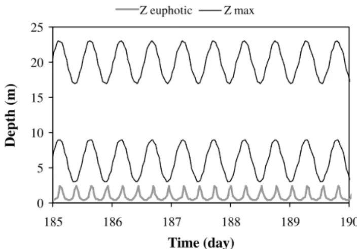
Fig. 3. Periodic forcing functions for the 1st set of simulations: water depthzmax. The average depth (i.e. the depth at mid-tide) is comprised between 6 m and 20 m, depending on the simulation. The tidal range is equal to 6 m in all cases. Euphotic depth, defined as the depth where 1% of the incident light is reached, is also repre-sented. It is computed from the forcing function (kd)of Fig. 2, and is identical for all simulations. It is always smaller than the water depthzmax.

surface is taken as a constant value (6%). The PAR fraction of the total incident solar light is equal to 50%. In the pres-ence of a cloud cover (CC, expressed as a fraction between 0 and 1), a cloudiness factor CT is taken into account, accord-ing to:

CT=1−0.585 CC (15)

(adapted from Vila et al., 1996). The grey line in Fig. 2 shows the temporal variation ofE0that has been used for the

sim-ulations. It is typical for a cloudless, summer period (4 to 9 July) at latitude 52◦N.

Following the hypothesis that the current velocity is the key control factor for SPM and turbidity, the resulting tidal variation of the light absorption coefficient kd is

approxi-mated by a sine function of period 6 h 12 min. This value cor-responds to half the period of the M2 tidal harmonic (black line, Fig. 2) and allows reproducing the occurrence of two turbidity minima per tidal cycle, corresponding to low- and high-water slacks. Conversely, two turbidity maxima are also simulated, for maximum ebb and flood velocities respec-tively. The values selected forkd(between 2 and 16 m−1) are

typical of turbid estuaries (Cloern, 1987). The resulting vari-ation of the euphotic depth (defined as the depth where PAR is equal to 1% of the surface value) is represented in Fig. 3. Finally, the water depthzmax is also modeled using a sine

function, but this time with a period 12 h 25 min and a tidal range equal to 6 m. A set of scenarios is considered, ranging from a relatively shallow reservoir (zmaxvarying between 3

and 9 m, average value=6 m) to deeper systems (zmax

0 500 1000 1500 2000

180 185 190 195 200 205 210 215

Time (day) E0

(µ

mol quanta.m

-2 .s -1 )

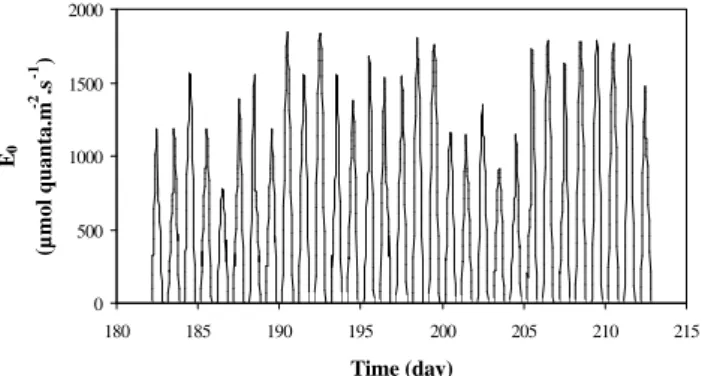
Fig. 4. Forcing function for the 2nd set of simulations: incident solar PARE₀(July 1999, 52◦N).

all cases, the euphotic depth, which varies between 0.3 and 2.3 m, represents only a small fraction of the total depthzmax.

In a second set of simulations, we introduce the influence of natural variability on the forcing functions E0, kd and zmax, and we investigate the consequence of this

variabil-ity on the primary production. Our purpose is to verify that the first-order features obtained in the previous set of simu-lations remain valid when more complex situations are de-scribed. By comparing the results of these simulations with experimental observations, we also aim at a validation of the model approach. The forcing functions are now parameter-ized from field data and from model results obtained for the Scheldt estuary (Belgium – The Netherlands), which can be considered as a typical example of a macro-tidal, turbid en-vironment (Wollast, 1988). Two situations are considered, which differ inkd as well as in zmax (the incident PARE0

being identical in both cases). The first situation corresponds to a shallow site (location 1, representative of the fresh water zone situated in the tidal estuary, about 110 km of the estu-arine mouth), while the second situation considers a deeper area of the estuary (location 2, typical of the brackish area around the harbour of Antwerp, km 80 from the estuarine mouth). ForE0(t ), the same astronomical routine as above

is used, but the resulting incident solar radiation is modified using a measured cloud coverage factor for temperate regions (July 1999, data supplied by IRM (1999), Fig. 4). The light attenuation coefficientkd(t )has been obtained from a large

number of vertical light profiles and SPM measurements con-ducted throughout 2002. It is expressed as an explicit func-tion of SPM:

kd=1.4+0.0592 SPM (16)

with kd in m−1 and SPM in mg.L−1 (Fig. 5). Note that

self-shading by the phytoplankton is not accounted for in the model. In our test system (the Scheldt estuary), it gener-ally plays a comparatively small role in the overall turbidity. Typical values of SPM concentration at the test sites are in the range 50–200 mg.L−1, whereas phytoplankton biomass is most of the time lower than 10 mg.L−1(dry weight).

Di-0 5 10 15

0 50 100 150 200

SPM (mg.L

)

k

(m

-1

)

Fig. 5.Linear relationship betweenkdand SPM as measured in the Scheldt estuary (k_d=1.4+0.0592×SPM;r2=0.609).

rect determination of the scalar absorption coefficientkdhas

also been performed, following a method adapted from Kirk (1994). Given that the vertical light profile is decreasing ex-ponentially, the value ofkdcan simply be obtained by

mea-suring the irradianceEdat two different depthsz1andz2: kd=

1 (z2−z1)

ln Ed(z1) Ed(z2)

. (17)

The in situ measurements have been made using two spher-ical quantum sensors (Aquamatic AQPL-UV912) separated by a constant, known vertical distance (∼50 cm). This tech-nique eliminates the need for incident light compensation and allows the continuous logging of thekd value. An example

of results for the Scheldt is given in Fig. 6. In addition, ver-tical profiles of scalar irradiance have repeatedly shown that thekdvalue can be considered as constant with depth in this

well-mixed estuary, at least in the euphotic layer (Fig. 7). In this second set of simulation, the SPM concentration is estimated using the concept of maximum transport capacity, which allows expressing the particulate matter content as a function of the local instantaneous current velocity and water depth (Verbanck, 2003):

SPM=X |u| z2

max 5

+Y , (18)

where|u|is the modulus of the cross-sectional averaged ve-locity and X, Y are two constants. The two variables u andzmaxare obtained from a one-dimensional hydrodynamic

2 4 6 8 10 12

06:00 08:00 10:00 12:00 14:00 16:00 18:00 20:00

Time (hh:mm)

kd

(m

-1 )

Continuous measurements From vertical profiles

Fig. 6. Time variation of the light extinction coefficient for scalar irradiance during a complete tidal cycle (km 115, 22 August 2002).

-8 -6 -4 -2 0

0 0.5 1 1.5

Depth (m)

ln (PAR . PAR

0

-1 )

Slack

Ebb tide

Fig. 7. Vertical profile of scalar irradiance measured in the tidal Scheldt estuary (km 115, 22 August 2002).

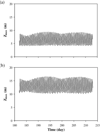
zmaxvaries during the tide between 4 m at low tide and 9 m

at high tide (tidal range=5 m); in the deeper area (Fig. 8b), these values are respectively equal to 10 m and 16 m (tidal range=6 m).

In Eq. (18) above, the constant termY corresponds to the finer particulate material, which remains in suspension in the water column (wash load). The coefficientY is essentially dependent on the nature of the suspension, which can vary along the estuarine gradient. In order to reproduce the SPM concentration range commonly observed in the two areas, distinct values for the constants (X,Y) have been used for the simulation:X=2×103andY=40 for the shallow, freshwater tidal estuary; X=6×103 andY=25 for the deeper, brackish region. The resulting variations ofkdfor both situations are

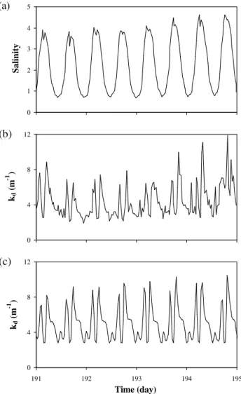
represented in Fig. 9. Despite its simplicity, this approach provides a realistic first-order description of the SPM and kd dynamics, as shown by the comparison between the

tur-bidity measured at a monitoring station located in a zone of high SPM content (km 80 from the mouth) and the results of a simulation carried out for the same location (Figs. 10b

0 5 10 15 20

Zmax

(m)

(a)

0 5 10 15 20

180 185 190 195 200 205 210 215

Time (day) Zmax

(m)

(b)

Fig. 8.Forcing function for the 2nd set of simulations: water depth zmax.(a)shallow area,(b)deeper area.

and 10c). Two peaks per tidal cycle can be observed, corre-sponding to maximum ebb and flow velocities. The very fast settling of suspended solids at slack water is another salient feature of the observed and modelled SPM dynamics.

Because the tidal velocities computed by the HD model are essentially similar in the shallow and deeper areas, the SPM, and hence the kd, differ mainly via the influence of zmax, according to Eq. (18). Comparing Figs. 9a and 9b

shows indeed that the resulting kd is on average higher at

the shallow site than at the deeper site. In both cases, the water depth and the light attenuation coefficient are strongly modulated by the spring-neap oscillations.

4 Dynamics of phytoplankton growth

4.1 First set of simulations

The results of the simulations obtained when using simple, periodic forcing functions forE0, kd andzmax are

synthe-sized in Figs. 11a to 11c. Figure 11a shows the time evolution of the PAR, immediately below the water surface (E0)and at

differ-0 5 10 15

kd

(m

-1 )

(a)

0 5 10 15

180 185 190 195 200 205 210 215

Time (day) kd

(m

-1 )

(b)

Fig. 9.Forcing function for the 2nd set of simulations: light attenu-ation coefficientkd.(a)shallow area,(b)deeper area.

ent from the purely sinusoidal signal at the surface. A com-plex, multiple-peak pattern is obtained, which results from the modulation ofE0(t )bykd(t ). Because these two signals

have different frequencies, the underwater PAR shows two or three daily peaks with a progressive phase shift in the daily maximum. This idealized simulation demonstrates that the maximum underwater PAR is most of the time not synchro-nized with solar noon: synchronism with solar noon (±1_/2h)

actually occurs every 6 to 7 days, as a result of the interaction between lunar (tide) and solar (night-day) forcing functions. Similar dynamics are predicted for the depth-integrated gross phytoplankton production (GPPz), as illustrated in Fig. 11b (black line) which represents a chlorophyll-specific value (GPPz divided by the chlorophyllaconcentration): us-ing this biomass-specific value removes the day-to-day vari-ation of integrated phytoplankton production due to biomass growth (or decay) . The resulting curve applies to each sim-ulation in the first set, because (a) the water depth is always greater than the euphotic depth and (b) the time variation of E0 andkd are identical in all cases. The computed pattern

is essentially similar to the one of PAR at 20 cm (Fig. 11a), although the differences between peak values within a given day are slightly less, a direct consequence of the non-linear relationship between GPP and PAR (Eq. 6). The simulation leads to the rather unexpected result that, in some instances (e.g. day 185), the highest instantaneous depth-integrated GPPz may occur at 9 a.m. and again at 3 p.m. (solar time),

0 1 2 3 4 5

Salinity

0 4 8 12

kd

(m

-1 )

0 4 8 12

191 192 193 194 195

Time (day) kd

(m

-1 )

(a)

(b)

(c)

Fig. 10. Variation of(a)salinity and(b)the light attenuation co-efficient as measured at a monitoring station in the Scheldt estuary (km 80, 10 to 14 July 1998). (c)Computed variation of the light attenuation coefficient (km 80, 10 to 14 July 1998).

although the incident solar light intensity is far from its max-imum at these moments.

A very different time pattern is predicted for GPPz if an averagekd value (i.e. the arithmetic mean over one tide) is

used for the simulation (Fig. 11b, grey line). As expected, chlorophyll-specific GPPz closely follows in this case the time evolution ofE0(t ). More importantly, the depth- and

time-integrated GPPzt is very different whether a time depen-dent or a constant, meankdvalue is used. In the latter case,

the integrated value is significantly lower, as it can be seen in Fig. 11c, which represents the chlorophyll-specific produc-tion, integrated over one day (24 h), computed for 5 consecu-tive days. The daily values obtained when using a variablekd

production equal to 41 gC.m.gChl−1_.day−1_{, an}

underestima-tion of 37 to 39% with respect to the former range of results. These large differences are of course due to the strongly non-linear (bi-exponential) relationship between GPP andkd

(Eqs. 6 and 12). Note that using an alternative averaging pro-cedure (i.e. using a geometric instead of an arithmetic mean) does not significantly improve the estimation of the daily GP-Pzt based on a constantkdvalue.

One may argue that sedimentation and resuspension mech-anisms, that control the SPM dynamics, could affect simi-larly phytoplankton cells. In some estuaries, short-term vari-ations of chlorophylla have been observed simultaneously with changes in turbidity (Demers et al., 1987; de Jonge and van den Bergs, 1987; Cloern et al., 1989; Litaker et al., 1993; Lucas, 2003). MacIntyre and Cullen (1996) even conclude that the decrease in mean irradiance caused by resuspension is compensated for by a concomitant increase in suspended chlorophylla, and hence has a negligible influence on GPPz estimates. However, chlorophylla resuspension is only re-ported in shallow estuaries (<2.5 m) or in the shallower ar-eas of deeper estuaries (such as tidal flats<60 cm), where benthic diatoms may often be found. In this paper, we exam-ine systems where the mixing depth is predominantly greater than the euphotic depth, a condition that is not extremely favourable to the development of benthic microalgae (Muy-laert et al., 2002). To verify this assumption, simultaneous measurements of turbidity and chlorophyllahave been per-formed at various depths in the Scheldt estuary (oligo- and mesohaline regions) during a number of tidal cycles. These measurements have never shown any strong, positive correla-tion between SPM and chlorophylla, suggesting that, in this type of environment, short-term variations in phytoplankton concentration are essentially due to the advection of water masses, rather than to phytoplankton settling and resuspen-sion.

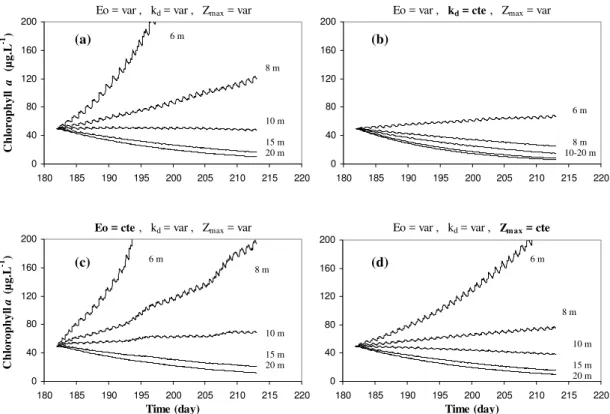
The influence of water depth on the net phytoplankton growth is illustrated in Fig. 12 for the whole set of scenar-ios. As the average depth increases, the processes responsi-ble for phytoplankton loss (maintenance respiration and mor-tality) become gradually predominant in the expression of r (Eq. 13). As a result, the phytoplankton biomass rapidly increases in the shallow reservoirs scenarios, while it ap-proaches an exponential decrease (typical of a first-order de-cay) in the deep reservoirs scenarios (Fig. 12a). Figure 12 also shows the effect of time-averaging the various forcing functions on the long-term trajectories of computed phyto-plankton biomass. As expected from previous results, the deviation between the varyingkdand the corresponding

con-stant kd cases may become exceedingly large in the long

term, because of the cumulative effect of the difference in phytoplankton growth (Figs. 12a and 12b). The trajectories are also increasingly divergent when the average water depth is decreasing. In the case of relatively shallow waters, ignor-ing the short term variability ofkdmay even lead to predict

a negative biomass growth instead of a positive one. In our

0 20 40 60 80

185 186 187 188 189 Time (day)

Chl-specific GPPzday _{(gC . m . gChl}

-1. day -1)

computed with time-varying kd computed with constant kd

0 5 10 15 20

185 186 187 188 189 190 Time (day)

Chl-specific GPPz _{(gC . m . gChl}

-1.h -1)

computed with time-varying kd computed with constant kd

0 500 1000 1500 2000

185 186 187 188 189 190 Time (day)

E (µ

mol quanta . m

-2 . s -1)

Eo PAR 20 cm

(a)

(b)

(c)

Fig. 11. First set of simulations, days 185 to 190 (4–9 July): (a)Incident solar light (PAR)E₀at the surface of the water col-umn and computed PAR at a 20 cm depth; (b) Depth-integrated, chlorophyll-specific gross primary production. The time variation of the biomass-specific GPPz is computed using a time-varyingkd value (black line) or a constant, time-averagedkdvalue (gray line); (c)Time- and depth-integrated, chlorophyll-specific gross primary production. The daily values of the biomass-specific GPPzt are computed using a time-varyingkdvalue (black bars) or a constant, time-averagedkdvalue (gray bars).

cases, it can be seen that the average depth under which vary-ing and constantkdmodels indicate an opposite sign for

Eo = var , kd = var , Zmax = cte

0 40 80 120 160 200

180 185 190 195 200 205 210 215 220

Time (day)

Eo = var , kd = cte , Zmax = var

0 40 80 120 160 200

180 185 190 195 200 205 210 215 220

Eo = cte , kd = var , Zmax = var

0 40 80 120 160 200

180 185 190 195 200 205 210 215 220

Time (day)

C

h

lo

ro

p

h

y

ll

a

(µ

g

.L

-1 )

Eo = var , kd = var , Zmax = var

0 40 80 120 160 200

180 185 190 195 200 205 210 215 220

C

h

lo

r

o

p

h

y

ll

a

(µ

g

.L

-1 )

(c) 6 m

8 m

20 m 15 m 10 m

(d) 6 m

8 m

20 m 15 m 10 m 6 m

8 m 10-20 m

(a) 6 m

8 m

20 m 15 m 10 m

(b)

Fig. 12. First set of simulations, days 182 to 212 (1–30 July): Evolution of the net algal biomass (expressed in chlorophylla) computed over a 30-days period for a range of bathymetry. The average depth (at mid-tide) is comprised between 6 m and 20 m, tidal range is equal to 6 m in all simulations.(a)All forcing functions (E0,kd,zmax)are varying with time;(b)Using a constant, time-averaged value for the light attenuation coefficientkd;(c)Using a constant, time-averaged value for the incident solar irradiance (PAR)E0;(d)Using a constant, time-averaged value for the water depthzmax.

model responses tend to vanish for an average depth greater than 15 m.

The model response to time-averaging irradiance (Fig. 12c) and water depth (Fig. 12d) has also been investi-gated. In the case of irradiance, simulations have been made applying a constant, mean E0 value for the length of the

light period and a null value at night. For constant water depth, mid-tide values have been used. The results show that neglecting the variability of the turbidity is by far the most important source of deviation in the estimation of net phytoplankton growth. Neglecting the tidal variation of the water depth also leads in our case to an underestimation of the net biomass growth, as already pointed out by Lucas and Cloern (2002), but the effect is not as strong as the former one and is only noticeable for average depths less than about 8 m. Finally, using an average irradiance leads to an overestimation, although this effect only takes some importance in the long term and in the shallowest systems. 4.2 Second set of simulations

The application of simplified periodic forcing functions to the case of a well-mixed, oscillating-depth reservoir gives a conceptual understanding of the coupling between sediment

dynamics, light climate in the water column and phytoplank-ton production. To advance one step further in the analysis, more complex forcing functions are now considered. They are typical of two locations within the Scheldt estuary, i.e. the brackish, deep area around the harbour of Antwerp (km 80) and the fresh water, shallow zone situated in the tidal es-tuary, about 40 km upstream from the former. Note that our purpose here is clearly not to develop a model of the Scheldt estuary, a task that would require to consider the complex lateral and longitudinal bathymetry of the estuary, as well as the role of transport mechanisms and mass exchanges in this complex system. We rather try to follow the same approach as the one used by Lucas et al. (1999a and b) in their study of the processes governing phytoplankton blooms in SSFB. Quoting these authors, we use the Scheldt as a “natural labo-ratory” and our model for “numerical experiments” in order to “gain insight into physical-biological mechanisms poten-tially important to a broad class of estuaries”.

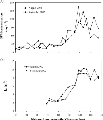
In the Scheldt estuary, longitudinal profiles of SPM and of kd result in a strong landwards decrease of the water

0 30 60 90 120 150 180

SPM concentration

(mg.L

-1 )

August 2002

September 2002

(a)

0 2 4 6 8 10 12

0 20 40 60 80 100 120 140 160

Distance from the mouth (Vlissingen; km)

kd

(m

-1 )

August 2002

September 2002

(b)

Fig. 13. Longitudinal distribution of(a)suspended solids concen-tration and(b)light attenuation coefficient along the Scheldt estu-ary. Location 1 (shallow area) is at km 120 and location 2 (deeper area) is at km 80.

when applying our reservoir model to both selected loca-tions, a positive net phytoplankton growth is predicted at the more turbid one (location 1, shallow site), whereas a negative net phytoplankton growth is simulated at location 2 (deeper site), in spite of the lower SPM concentration (Fig. 14, kd-v curves). In the absence of longitudinal transport, our model predicts a three-fold increase in algal biomass (expressed as chlorophyllaconcentration) over a one-month period at lo-cation 1. In contrast, the chlorophyllavalue is reduced by a factor of about 30% at location 2 within the same period. The main reason for this behaviour originates from the difference of bathymetry at both sites, location 2 displaying an aver-age water depth approximately twice as large as the value at location 1. Although our purpose is not to model the lon-gitudinal phytoplankton gradient in the estuary, we can as-sociate these results with field measurements of chlorophyll aconcentrations in the Scheldt estuary. Indeed, an increas-ing biomass concentration in the seaward direction is only possible if the depth-integrated phytoplankton growth, as es-timated with the present zero-dimensional model, is positive. This is a necessary, but not a sufficient condition. How-ever, a negative depth-integrated phytoplankton growth in the model will always result in a decreasing concentration gradi-ent. Model results are thus not in contradiction with the rapid drop in chlorophyllaconcentration that is observed between the two locations (Fig. 15).

0 20 40 60 80 100 120 140

180 190 200 210 220

Time (day)

Chlorophyll

a

(µ

g . L

-1)

Shallow site

Deeper site

kd-v

kd-v

kd-c

kd-c

Fig. 14. Second set of simulations, days 182 to 212 (1–30 July): Net chlorophyllaevolution during a 30-day simulation for the shal-low area and for the deeper area. Simulations have been performed using time-varyingkd (kd-v curves), and time-averagedkd (kd-c curves).

0 50 100 150 200 250 300 350

0 20 40 60 80 100 120 140 160

Distance from the mouth (Vlissingen; km)

Chlorophyll

a

(µ

g.L

-1 )

July 2002 August 2002

September 2002

Fig. 15. Longitudinal profile of chlorophyllaconcentration along the Scheldt estuary. Location 1 (shallow area) is at km 120 and location 2 (deeper area) is at km 80.

Figure 14 also displays the results of the 30-day simula-tion when a constant, time-averagedkdis used (kd-c curves).

Once again, the net phytoplankton growth exhibits a nega-tive deviation, especially at the shallow site. However, this effect is not strong enough to cause a shift from net biomass growth to net biomass decay, at least in a system where trans-port processes are not taken into account.

model predicts a four-fold increase in algal biomass over a one-month period at location 1 (shallow site), and a slight decrease in chlorophylla at location 2 (deeper site). How-ever, if photosynthetic parameters exhibit a minimum value at noon, then chlorophylla concentration increases by only 50% at location 1 over a month, and it decreases by 50% at location 2. Depending on the diel pattern taken into ac-count, photoacclimation may thus enhance or reduce the phy-toplankton production. In a more elaborate model of the phytoplankton distribution along the estuary, where transport processes are considered, this may even make the difference between positive and negative population growth at a partic-ular location. Finally, note that the harmonic coupling be-tweenαB,P_maxB andkd slightly amplifies the importance of

using a time-dependentkdinstead of a constant mean value.

It has already been shown (see 1st set of simulations) that the daily integrated GPPzt computed with a time-dependent kd was about 37% higher than the value obtained using an

average kd. When considering a diel-variation of αB and P_maxB , this difference between the daily integrated GPPzt’s increases from 37 to 40% when photosynthetic parameters exhibit their minimum value at noon, and to 41% when they exhibit a peak at noon.

5 Conclusions

A number of hypothesis have been invoked to explain the well recognized phytoplankton decay that is often observed along the longitudinal salinity gradient of turbid, macro-tidal estuaries. Among those, factors such as salinity stress, zoo-plankton grazing and light limitation due to the presence of a turbidity maximum, have been advocated (Soetaert et al., 1994; Kromkamp and Peene, 1995; Vanderborght et al., 2002). In this paper, we have applied a simple model to assess the net phytoplankton growth in a system charac-terized by high-frequency variations of the physical forcing functions. In this type of system, it is difficult to draw in-tuitive conclusions about the phytoplankton production-loss balance, because of the complex interactions involved. Sim-ulation results show that, in shallow to moderately deep sys-tems (<15 m), this balance is strongly affected by the short-term (∼hourly) fluctuations of the light regime, in particu-lar by those linked to the tidal dynamics of SPM. We have also demonstrated that the interplay between tidal and ny-chtemeral oscillations has to be resolved at least at the hourly timescale. This is a direct consequence of the different fre-quencies of the physical forcing functions (E0, kd, zmax),

which results in a complex pattern of phytoplankton produc-tion at this timescale. Comparison between simulaproduc-tions using temporally resolved and averaged forcing functions indicate that the latter approach leads to significant errors in the es-timation of estuarine productivity, especially in turbid and shallow areas (<8m).

Acknowledgements. We thank D. Bajura, M. Loijens and

N. Roevros for their participation in analytical work and field mis-sions. We also thank K. Muylaert and two anonymous reviewers for their constructive feedback. The support of the “Administratie Wa-terwegen en Zeewezen” of the Ministry of the Flemish Community and of the MUMM (Management Unit of the Mathematical Model of the North Sea, Royal Belgian Institute of Natural Sciences) is gratefully acknowledged. This research has been supported by the E.U. project EUROTROPH (EVK3-CT-2000-00040). The Belgian FRIA (“Fonds pour la Recherche dans l’Industrie et l’Agriculture”) and the “Fondation Baron Van Buuren” have granted the work of one of the authors (X.D.).

Edited by: J. Middelburg

References

Boyer, J. N., Christian, R. R., and Stanley, D. W.: Patterns of phyto-plankton primary productivity in the Neuse River estuary, North Carolina, USA, Mar. Ecol. Prog. Ser., 97, 287–297, 1993. Cloern, J. E.: Turbidity as a control on phytoplankton biomass and

productivity in estuaries, Cont. Shelf Res., 7, 1367–1381, 1987. Cloern, J. E., Powell, T. M., and Huzzey, L. M.: Spatial and

tem-poral variability in South San Francisco Bay (USA), II. Tempo-ral changes in salinity, suspended sediments, and phytoplankton biomass and productivity over tidal time scales, Estuarine, Coast. Shelf Sci., 28, 599–613, 1989.

Cole, B. E.: Temporal and spatial patterns of phytoplankton produc-tion in Tomales Bay, California, USA, Estuarine, Coast. Shelf Sci., 28, 103–115, 1989.

Cole, B. E. and Cloern, J. E.: Significance of biomass and light availability to phytoplankton productivity in San Francisco Bay, Mar. Ecol. Prog. Ser., 17, 15–24, 1984.

Cole, B. E. and Cloern, J. E.: An empirical model for estimating phytoplankton productivity in estuaries, Mar. Ecol. Prog. Ser., 36, 299–305, 1987.

Cole, J. J., Caraco, N. F., and Peierls, B. L.: Can phytoplankton maintain a positive carbon balance in a turbid, freshwater, tidal estuary?, Limnology and Oceanography, 37, 1608–1617, 1992. Cullen, J. J. and Lewis, M. R.: The kinetics of algal photoadaptation

in the context of vertical mixing, J. Plankt. Res., 10, 1039–1063, 1988.

de Jonge, V. N. and van den Bergs, J.: Experiments on the resus-pension of estuarine sediments containing benthic diatoms, Es-tuarine, Coast. Shelf Sci., 24, 725–740, 1987.

Demers, S., Legendre, L., and Therriault, J.-C.: Phytoplankton re-sponses to vertical tidal mixing, in: Tidal mixing and plankton dynamics, edited by: Bowman, J., Yentsch, M., and Peterson W. T., Springer-Verlag, Berlin – Heidelberg, 1986.

Demers, S., Therriault, J.-C., Bourget, E., and Abdourrahmane, B.: Resuspension in the shallow sublittoral zone of a macrotidal es-tuarine environment: wind influence, Limnology and Oceanog-raphy, 32, 327–339, 1987.

Di Toro, D. M.: Optics of turbid estuarine waters: approximation and application, Water Res., 12, 1059–1068, 1978.

Falkowski, P. G. and Raven, J. A.: Aquatic Photosynthesis, Black-well Science Ltd., 1997.

Deep-Sea Research I, 42, 1111–1149, 1995.

Fasham, M. J. R., Ducklow, H., and McKelvie, S. M.: A nitrogen-based model of plankton dynamics in the oceanic mixed layer, J. Mar. Res., 48, 591–639, 1990.

Fettweis, M., Sas, M., and Monbaliu, J.: Seasonal, neap-spring and tidal variation of cohesive sediment concentration in the Scheldt estuary, Belgium, Estuarine, Coast. Shelf Sci., 47, 21–36, 1998. Fichez, R., Jickells, T. D., and Edmunds, H. M.: Algal blooms in

high turbidity, a result of the conflicting consequences of turbu-lence on nutrient cycling in a shallow water estuary, Estuarine, Coast. Shelf Sci., 35, 577–592, 1992.

Geider, R. J., MacIntyre, H. L., and Kana, T. M.: A dynamic model of photoadaptation in phytoplankton, Limnology and Oceanog-raphy, 41, 1–15, 1996.

Geider, R. J., MacIntyre, H. L., and Kana, T. M.: Dynamic model of phytoplankton growth and acclimation: responses of the bal-anced growth rate and the chlorophyll a:carbon ratio to light, nutrient-limitation and temperature, Mar. Ecol. Prog. Ser., 148, 187–200, 1997.

Geider, R. J., MacIntyre, H. L., and Kana, T. M.: A dynamic reg-ulatory model of phytoplanktonic acclimation to light, nutrients, and temperature, Limnology and Oceanography, 43, 679–694, 1998.

Gilstad, M., Johnsen, G., and Sakshaug, E.: Photosynthetic param-eters, pigment composition and respiration rates of the marine diatom Skeletonema Costatum grown in continuous light and a 12:12 h light-dark cycle, J. Plankt. Res., 15, 939–951, 1993. Grobbelaar, J. U.: Phytoplankton productivity in turbid waters, J.

Plankt. Res., 7, 653–663, 1985.

Han, B.-P.: A mechanistic model of algal photoinhibition induced by photodamage to photosystem-II, J. Theor. Biol., 214, 519– 527, 2002.

Hansell, D. A. and Carlson, C. A.: Net community production of dissolved organic carbon, Global Biogeochemical Cycles, 12, 443–453, 1998.

Harding, L. W. J., Meeson, B. W., and Fisher, T. R. J.: Phytoplank-ton production in two east coast estuaries: photosynthesis-light functions and patterns of carbon assimilation in Chesapeake and Delaware Bays, Estuarine, Coast. Shelf Sci., 23, 773–806, 1986. Heip, C. H. R., Goosen, N., Herman, P. M. J., Kromkamp, J., Mid-delburg, J. J., and Soetaert, K.: Production and consumption of biological particles in temperate tidal estuaries, Oceanography and Marine Biology: an Annual Review, 33, 1–149, 1995. Irigoien, X. and Castel, J.: Light limitation and distribution of

chlorophyll pigments in a highly turbid estuary: the Gironde (SW France), Estuarine, Coast. Shelf Sci., 44, 507–517, 1997. I.R.M.: Bulletin Mensuel des Observations Climatologiques de

l’Institut Royal M´et´eorologique de Belgique, Juillet 1999, par-tie II, edited by: Malcorps, H., 1999.

Kana, T. M., Geider, R. J. and Critchley, C.: Regulation of pho-tosynthetic pigments in micro-algae by multiple environmental factors: a dynamic balance hypothesis, New Phytologist, 137, 629–638, 1997.

Keller, A. A.: Estimating phytoplankton productivity from light availability and biomass in the MERL mesocosms and Narra-gansett Bay, Mar. Ecol. Prog. Ser., 45, 159–168, 1988.

Kirk, J. T. O.: Light and photosynthesis in aquatic ecosystems, 2nd edn. Cambridge University Press, 1994.

Kromkamp, J. and Peene, J.: Possibility of net phytoplankton

pri-mary production in the turbid Schelde Estuary (SW Nether-lands), Mar. Ecol. Prog. Ser., 121, 249–259, 1995.

Kromkamp, J., Peene, J., van Rijswijk, P., Sandee, A., and Goosen, N.: Nutrients, light and primary production by phytoplankton and microphytobenthos in the eutrophic, turbid Westerschelde estuary (The Netherlands), Hydrobiologia, 311, 9–19, 1995. Lancelot, C., Hannon, E., Becquevort, S., Veth, C., and de Baar, H.

J. W.: Modeling phytoplankton blooms and carbon export pro-duction in the Southern Ocean: dominant controls by light and iron in the Atlantic sector in Austral spring 1992, Deep-Sea Re-search I, 47, 1621–1662, 2000.

Lancelot, C., Mathot, S., and Owens, N. J. P.: Modelling protein synthesis, a step to an accurate estimate of net primary produc-tion: Phaeocystis pouchetii colonies in Belgian coastal waters, Mar. Ecol. Prog. Ser., 32, 193–202, 1986.

Lancelot, C., Veth, C., and Mathot, S.: Modelling ice-edge phy-topankton bloom in the Scotia-Weddell sea sector of the South-ern Ocean during spring 1988, J. Mar. Sci., 2, 333–346, 1991. Langdon, C.: On the causes of interspecific differences in the

growth-irradiance relationship for phytoplankton, II. A general review, J. Plankt. Res., 10, 1291–1312, 1988.

Langdon, C.: The significance of respiration in production mea-surements based on oxygen, ICES Mar. Sci. Symp., 197, 69–78, 1993.

Lewitus, A. J. and. Kana, T. M.: Light respiration in six estuar-ine phytoplankton species: contrasts under photoautotrophic and mixotrophic growth conditions, J. Phycol., 31, 754–761, 1995. Litaker, W., Duke, C. S., Kenney, B. E., and Ramus, J.:

Short-term environmental variability and phytoplankton abundance in a shallow tidal estuary, II. Spring and fall, Mar. Ecol. Prog. Ser., 94, 141–154, 1993.

Lucas, C. H.: Observations of resuspended diatoms in the turbid tidal edge, J. Sea Res., 50, 301–308, 2003.

Lucas, L. V. and Cloern, J. E.: Effects of tidal shallowing and deep-ening on phytoplankton production dynamics: a modeling study, Estuaries, 25, 497–507, 2002.

Lucas, L. V., Koseff, J. R., Cloern, J. E., Monismith, S. G., and Thompson, J. K.: Processes governing phytoplankton blooms in estuaries, I. The local producion-loss balance, Mar. Ecol. Prog. Ser., 187, 1–15, 1999a.

Lucas, L. V., Koseff, J. R., Monismith, S. G., Cloern, J. E., and Thompson, J. K.: Processes governing phytoplankton blooms in estuaries, II. The role of horizontal transport, Mar. Ecol. Prog. Ser., 187, 17–30, 1999b.

Macedo, M. F., Ferreira, J. G., and Duarte, P.: Dynamic behaviour of photosynthesis-irradiance curves determined from oxygen production during variable incubation periods, Mar. Ecol. Prog. Ser., 165, 31–43, 1998.

MacIntyre, H. L. and Cullen, J. J.: Primary production by sus-pended and benthic microalgae in a turbid estuary: time-scales of variability in San Antonio Bay, Texas, Mar. Ecol. Prog. Ser., 145, 245–268, 1996.

MacIntyre, H. L., Kana, T. M., Anning, T., and Geider, R. J.: Pho-toacclimation of photosynthesis irradiance response curves and photosynthetic pigments in microalgae and cyanobacteria (Re-view), J. Phycol., 38, 17–38, 2002.

Malinsky-Rushansky, N. Z. and Legrand, C.: Excretion of dis-solved organic carbon by phytoplankton of different sizes and subsequent bacterial uptake, Mar. Ecol. Prog. Ser., 132, 249–255, 1996.

Mallin, M. A. and Paerl, H. W.: Effects of variable irradiance on phytoplankton productivity in shallow estuaries, Limnology and Oceanography, 37, 54–62, 1992.

May, C. L., Koseff, J. R., Lucas, L. V., Cloern, J. E., and Schoell-hamer, D. H.: Effects of spatial and temporal variability of tur-bidity on phytoplankton blooms, Mar. Ecol. Prog. Ser., 254, 111– 128, 2003.

Meeus, J.: Astronomical algorithms, Willmann-Bell, Richmond, 2nd ed., 477 p., 1999.

Melis, A.: Photosystem-II damage and repair cycle in chloroplasts: what modulates the rate of photodamage in vivo?, Trends in Plant Science, 4, 130–135, 1999.

Mor´an, X. A. G. and Estrada, M.: Phytoplanktonic DOC and POC production in the Bransfield and Gerlache Straits as derived from kinetic experiments of14C incorporation, Deep-Sea Research II, 49, 769–786, 2002.

Muylaert, K., Van Nieuwerburgh, L., Sabbe, K., and Vyverman, W.: Microphytobenthos communities of the brackish to freshwater tidal reaches of the Schelde estuary (Belgium), Belgian Journal of Botany, 135, 15–26, 2002.

Otero, A. and Vincenzini, M.: Nostoc (cyanophyceae) goes nude: extracellular polysaccharides serve as a sink for reducing power under unbalanced C/N metabolism, J. Phycol., 40, 74–81, 2004. Pahl-Wostl, C. and Imboden, D.M.: DYPHORA – a dynamic model for the rate of photosynthesis of algae, J. Plankt. Res., 12, 1207– 1221, 1990.

Platt, T., Gallegos, C. L., and Harrison, W. G.: Photoinhibition of photosynthesis in natural assemblages of marine phytoplankton, J. Mar. Res., 38, 687–701, 1980.

Postma, H.: Sediment transport and sedimentation, in: Chemistry and Biogeochemistry of Estuaries, edited by: Olausson, E. and Cato, I., John Wiley and Sons Ltd., 153–186, 1980.

Pr´ezelin, B. B.: Diel periodicity in phytoplankton productivity, Hy-drobiologia, 238, 1–35, 1992.

Regnier, P., Mouchet, A., Wollast, R., and Ronday, F.: A discussion of methods for estimating residual fluxes in strong tidal estuaries, Cont. Shelf Res., 18, 1543–1571, 1998.

Regnier, P. and Steefel, C. I.: A high resolution estimate of the inorganic nitrogen flux from the Scheldt estuary to the coastal North Sea during a nitrogen-limited algal bloom, spring 1995, Geochimica et Cosmochimica Acta, 63, 1359–1374, 1999. Reid, P. C., Lancelot, C., Gieskes, W. W. C., Hagmeier, E., and

Weichart, G.: Phytoplankton of The North Sea and its dynamics: a review, J. Sea Res., 26, 295–331, 1990.

Soetaert, K., Herman, P. M. J., and Kromkamp, J.: Living in the twilight: estimating net phytoplankton growth in the Wester-schelde estuary (The Netherlands) by means of an ecosystem model (MOSES), J. Plankt. Res., 16, 1277–1301, 1994. Steemann Nielsen, E. and Hansen, V. Kr.: Measurements with the

carbon-14 technique of the respiration rates in natural popula-tions of phytoplankton, Deep-Sea Research I, 5, 222–233, 1959. Sverdrup, H. U.: On conditions for the vernal blooming of

phyto-plankton, J. Cons. Explor. Mer., 18, 287–295, 1953.

Vanderborght, J. P., Wollast, R., Loijens, M., and Regnier, P.: Ap-plication of a transport-reaction model to the estimation of bio-gas fluxes in the Scheldt estuary, Biogeochemistry, 59, 207–237, 2002.

Verbanck, M.: Sediment-laden flows over fully-developed bed-forms: first and second harmonics in a shallow, pseudo-2D tur-bulence environment, in: Shallow Flows, edited by: Jirka, G. H and Uijttewaal, W. S. J., TU Delft, II 231-II 236, 2003.

Vila, X., Colomer, J., and Garcia-Gil, L. J.: Modelling spectral irra-diance in freshwater in relation to phytoplankton and solar radi-ation, Ecological Modelling, 87, 59–68, 1996.

Weger, H. G., Herzig, R., Falkowski, P. G., and Turpin, D. H.: Res-piratory losses in the light in a marine diatom: measurements by short-term mass spectrometry, Limnology and Oceanography, 34, 1153–1161, 1989.

Williams, P. J. l. and Lef`evre, D.: Algal 14C and total carbon metabolisms, 1. Models to account for the physiological pro-cesses of respiration and recycling, J. Plankt. Res., 18, 1941– 1959, 1996.

Wofsy, S. C.: A simple model to predict extinction coefficients and phytoplankton biomass in eutrophic waters, Limnology and Oceanography, 28, 1144–1155, 1983.