TECHNIQUES AND ITS FIELD VALIDATION
Umidade do solo obtida por técnicas de mapeamento digital e sua validação de campo
Bruno Montoani Silva1, Sérgio Henrique Godinho Silva2, Geraldo Cesár de Oliveira1, Petrus Hubertus Caspar Rosa Peters1, Walbert Júnior Reis dos Santos3, Nilton Curi1
ABSTRACT
Digital techniques and tools can assist not only in the prediction of soil properties, such as soil moisture, but also in planning the use and management of areas for agriculture and, or, environmental purposes. In this sense, this work aimed to study wetness
indexes methods, defining the spatial resolution and selecting the estimation method that best correlates with water content data measured in the field, evaluating even moisture at different soil depths and seasons. This study was developed in a landscape with
strongly undulated relief and covered with Nitosols at the summit and upper middle third, and Argisols at the low middle third, ranging in altitude from 845 to 890 m, located in the southern state of Minas Gerais, Brazil. It were performed analyses of Pearson
linear correlation between soil moisture determined in the field, at depths of 10, 20, 30, 40, 60 and 100 cm and the water storage in 0-100 cm depth, and the topographic and SAGA wetness indexes, TWI and SWI, respectively, obtained from digital elevation models at different spatial resolutions. In most studied conditions, the TWI with resolution of 10 m provided better results, particularly for the dry season. In this study, only the depth of 100 cm resulted in a significant and positive correlation, suggesting that the moisture
levels are suitable for water dynamic studies in the subsurface, assisting in studies of hydrological dynamics and planning the soil use and management, especially for perennial plants with deeper root systems.
Index terms: Terrain attributes, soil water content determination, relief, water dynamics.
RESUMO
Técnicas e ferramentas digitais podem auxiliar na predição de propriedades do solo, a exemplo da umidade do solo, auxiliando no planejamento do uso e manejo de áreas com fins agrícolas e/ou ambientais. Nesse sentido, objetivou-se estudar índices de umidade, definir a resolução espacial e selecionar o método de estimativa que melhor se correlaciona com dados de teor de água medidos em campo, avaliando-se, ainda, a umidade em diferentes profundidades do solo e épocas do ano. Este estudo foi desenvolvido em uma paisagem com relevo forte ondulado e recoberta por Nitossolo no topo e no terço médio superior, e Argissolo no terço médio inferior, em altitude variando de 845 a 890 m, no sul do Estado de Minas Gerais, Brasil. Foram realizadas análises de correlação linear de Pearson entre a umidade do solo determinada em campo, nas profundidades de 10, 20, 30, 40, 60 e 100 cm além do armazenamento de água na camada 0-100 cm, e os índices de umidade TWI (índice topográfico de umidade) e SWI (índice de umidade SAGA) obtidos a partir de modelos digitais de elevação em diferentes resoluções espaciais. Na maioria das situações estudadas, o índice TWI com resolução de 10 m condicionou melhores resultados, particularmente no período seco do ano. Neste estudo, apenas para a profundidade de 100 cm houve correlação positiva e significativa, sugerindo que os índices de umidade são indicados para estudos de dinâmica da água em subsuperfície, auxiliando nos estudos de dinâmica hidrológica e no planejamento
de uso e manejo do solo, especialmente no caso de plantas perenes com sistema radicular mais profundo.
Termos para indexação: Atributos de terreno, determinação do conteúdo de água no solo, relevo, dinâmica da água.
1Universidade Federal de Lavras/UFLA – Departamento de Ciência do Solo/DCS – Lavras – MG – Brasil
2Universidade Federal de Lavras/UFLA – Departamento de Ciência do Solo/DCS – Cx. P. 3037 – 37200000 – Lavras – MG – Brasil – [email protected] 3Companhia de Desenvolvimento dos Vales do São Francisco e Parnaíba – CODEVASF – Montes Claros – MG
Received in october 23, 2013 and approved in november 22, 2013
INTRODUCTION
The emergence of new digital tools and techniques has aided in the prediction of the behavior of soils and their attributes and has contributed to a better understanding of the soil-landscape relationships. From digital elevation models (DEM) it has been possible to create the so-called terrain attributes, which are environmental variables representative of the relief, such as slope, curvature and wetness index, and that provide increasing application
on digital soil mapping (Lagacherie; McBratney, 2007; McBratney; Mendonça-Santos; Minasny, 2003).
use of alternative methods for generating DEMs with better quality. In the absence of more detailed DEMs, the user can build your own digital model (Pilesjö; Persson; Harrie, 2006).
There are several studies comparing the accuracy of DEMs from different sources and resolutions. In addition, currently there are several methodologies suitable for creating digital elevation models of better resolutions, such as those that use scanning contours, interpolation of elevation points or remote sensors (Pinheiro et al., 2012). Thompson; Bell and Butler (2001) evaluated the effect of the accuracy of different resolution DEMs and found out that models with poorer resolutions (larger cells) represent steeper areas as being of lower slopes and the flatter areas as being more hilly, not accurately portraying the characteristics observed in the field. Weihua and Montgomery (1994) were able to substantially improve the representation of relief with a DEM of 10 m resolution, compared to DEMs of 30 m and 90 m, however, the models with a resolution of 2 m and 4 m just slightly improved the 10 m DEM. Wilson; Repetto; Snyder (2000) demonstrated the impact that spatial resolution has on hydrological studies when they noted the drastic changes in length of rivers and recharge area maps by increasing the cell size of the DEM from 30 m to 200 m.
The correlations between terrain attributes and field data are important in verifying the accuracy of these digital representations of the landscape and in determining the appropriate size of the cells that make up the DEM (Florinsky; Kuryakova, 2000). Some of the terrain attributes most commonly used in digital soil mapping are: slope, aspect, curvature and wetness index. The representation of the moisture content can be made by the topographic wetness index (TWI), which has been widely used in estimating soil moisture, its spatial distribution (Grabs et al., 2009), and water flow in the subsurface at a given landscape (Zinko et al., 2005). TWI was developed by Beven and Kirkby (1979) and is defined by ln (a/tan β), where a is the upslope contributing area per unit contour length and tan β is the local slope gradient for estimating a hydraulic gradient.
In more recent works, the SAGA wetness index (SWI), created through the software SAGA GIS (Böhner; Conrad, 2009), has been used, even replacing the TWI, because it enables the adjustment of the uni to multidirectional convergence flow (Menezes, 2011). Anyway, both indexes have the function of identifying the characteristics of the water flow in the landscape (Sumfleth; Duttman, 2008), where higher values indicate areas most
likely to present saturated conditions, commonly found in the depressions and converging landscape, associated with low soil hydraulic conductivity (Beven; Wood, 1983). However, beyond indicating areas with higher potential soil moisture, it may be necessary to identify the correlation between the values of these indexes with the actual water content in the soil, aiding to define the most appropriate uses of this natural resource and adequate locations for placing hydrological studies. Also, the real precision of the soil moisture obtained from those indexes can be verified by validation methods in the field.
Once the knowledge about the local of the landscape associated with each soil type can define the potential water storage in a portion of a given soil toposequence, information regarding moisture levels are extremely important in planning the use and management of the area, because water is a major factor of production. Thus, the use of tools that assist in obtaining this information efficiently is encouraged, given the high cost and considerable time spent on monitoring soil moisture.
In this context, the objectives of this study were: (1) to find out which spatial resolution and method to estimate the soil water content best correlate with water content data measured in the field, and (2) to assess the season of the year and the soil depths that these correlations are significant.
MATERIAL AND METHODS Study Area
The study area is located in Bom Sucesso county, in Minas Gerais State, at the coordinates 21°06’50’’S and 44°49’22.35”W, with altitude ranging from 845 to 890 m and average slope of 25%. The region climate is Cwb, according to the Köppen classification, with cold and dry winters and hot and rainy summers, average annual rainfall around 1500 mm. The study area occupies 1.6 ha and has being cultivated with Australian cedar (Toona ciliata) for 2 years. The occurring soil
types are Nitosols and Argisols (Embrapa, 2013), located, respectively, on the steep and gently undulated portions of the landscape.
Evaluation of the soil moisture in the field
question and more details can be seen in Peters et al. (2013). Assessments of soil moisture were conducted in the dry season (19/09/2012) and in the rainy season (21/12/2012).
Digital Elevation Models
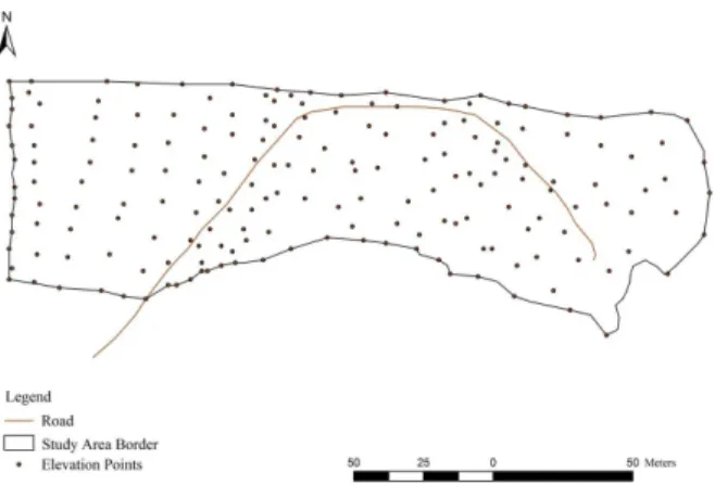
In the study area data of 190 elevation points were collected, forming a grid, with a distance of 8 meters between the points (Figure 1), using a calibrated altimeter, aiming at the creation of six digital elevation models (DEMs) in different resolutions: 0.5 m, 1 m, 3 m, 5 m, 10 m, and 15 m. At each elevation point, the geographic coordinates were obtained using a handheld GPS. The collected elevation data were interpolated using the tool Topo to Raster in ArcGIS 9.3 (ESRI) software, being then transformed into hydrologically consistent DEMs by the function fill sinks in SAGA GIS software (Böhner; Conrad, 2009).
identify the influence of the volume of water stored in the soil in relation to the wetness indexes, depending on the sampling dates and the soil depths. It was also calculated the water storage for the 0-100 cm layer with the purpose of comparing the wetness indexes generated by the software SAGA GIS.
The wetness indexes accuracy was assessed by Pearson linear correlation analysis between the generated indexes values and soil moisture measured by the probe, which was performed using the software SigmaPlot (version 10.0, Systat Software, San Jose, CA).
RESULTS AND DISCUSSION
Regardless the depth evaluated in the soil, the season of the year and the employed methods (SWI and TWI) (Table 1), the best DEMs resolutions did not satisfactory corresponded to the best results due to the absence of significant correlation between the predicted wetness indexes and moisture measured in the field with multisensor probes, although the higher resolutions provide more details (Stein; Riley; Halberg, 2001). It suggests that, despite the improvement in spatial resolution increases the amount of details on the maps, in regard to soil moisture, very high resolutions may complicate the data explanation as found out in this study. Thus, high resolution DEMs are not always necessary, as has been reported by Thompson; Bell and Butler (2001) in a study aiming to predict the spatial distribution of the A horizon depth. In that work, the authors found out that DEMs with better resolutions provided almost no gain in information, suggesting that, depending on the soil property being studied, less refined DEMs can provide adequate results.
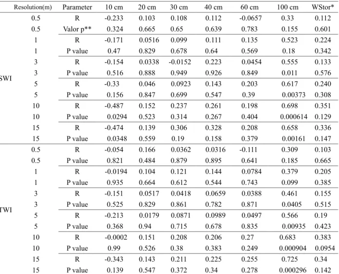
The highest correlation coefficient (0.725) and highly significant (p <0.01) was found for the dry season and obtained by the TWI method with a resolution of 15 m to a depth of 100 cm (Table 1). For the rainy season, the highest correlation was also found for the TWI method and 100 cm depth, but with a resolution of 10 m, resulting, in this case, in a correlation of 0.712, which is also highly significant (Table 2).
In the evaluation of the season in which the wetness indexes were better suited, for both methods the highest correlation occurred for indexes correlated with field data collected in the dry season (Table 1), with no substantial precipitation and surface runoff interference, thus being the soil moisture the result of the balance between capillary rise, evapotranspiration and deep drainage (Ghiberto et al., 2011; Reichardt; Timm, 2004).
Figura 1 – Elevation points distribution in the study area.
Wetness Indexes
Table 1 – Correlation coefficient (R) and significance of the correlation (p) between the TWI and SWI obtained from different DEM resolutions and soil moisture at different depths in the dry season.
Resolution(m) Parameter 10 cm 20 cm 30 cm 40 cm 60 cm 100 cm WStor*
SWI
0.5 R -0.233 0.103 0.108 0.112 -0.0657 0.33 0.112
0.5 Valor p** 0.324 0.665 0.65 0.639 0.783 0.155 0.601
1 R -0.171 0.0516 0.099 0.111 0.135 0.523 0.224
1 P value 0.47 0.829 0.678 0.64 0.569 0.18 0.342
3 R -0.154 0.0338 -0.0152 0.223 0.0454 0.555 0.133
3 P value 0.516 0.888 0.949 0.926 0.849 0.011 0.576
5 R -0.33 0.046 0.0923 0.143 0.203 0.617 0.240
5 P value 0.156 0.847 0.699 0.547 0.39 0.00373 0.308
10 R -0.487 0.152 0.237 0.261 0.198 0.698 0.351
10 P value 0.0294 0.523 0.314 0.267 0.404 0.000614 0.129
15 R -0.474 0.139 0.306 0.328 0.208 0.658 0.336
15 P value 0.0348 0.559 0.19 0.158 0.379 0.00161 0.147
TWI
0.5 R -0.054 0.166 0.0362 0.0316 -0.111 0.309 0.103
0.5 P value 0.821 0.484 0.879 0.895 0.641 0.185 0.665
1 R -0.0194 0.104 0.121 0.144 0.0784 0.379 0.205
1 P value 0.935 0.664 0.612 0.544 0.743 0.099 0.385
3 R -0.151 0.0517 0.0418 0.0659 0.0388 0.461 0.155
3 P value 0.525 0.829 0.861 0.782 0.871 0.0405 0.515
5 R -0.213 0.0179 0.0871 0.0989 0.0497 0.566 0.19
5 P value 0.368 0.94 0.715 0.678 0.835 0.00935 0.423
10 R -0.0002 0.151 0.208 0.206 0.27 0.683 0.383
10 P value 0.99 0.526 0.38 0.383 0.249 0.000904 0.0954
15 R -0.343 0.143 0.211 0.225 0.255 0.725 0.34
15 P value 0.139 0.547 0.372 0.34 0.278 0.000296 0.142
*Water storage at 0-100 cm depth. **Statistical significance, p value is significant at 5% when inferior to 0.05, and significant at 1% when p value is inferior to 0.01.
The best results obtained with the SWI method for both dry and wet seasons were also estimated by the 10 m resolution DEM, and also with the moisture data at 100 cm depth, obtaining, in such cases, correlations of 0.698 and 0.602, respectively. These results are highly significant (p <0.01), which confirms the trend of the 10 m DEM to be the one that best represents the relief in the study area. With regard to the water storage in 0-100 cm depth (Tables 1 and 2), there were no significant correlations with the wetness indexes, independently of the obtaining method and the DEM resolution.
For the soil moisture at a depth of 10 cm, it were observed significant correlations (p <0.05),
although negative, with the SWI for both dry and wet seasons in resolutions of 10 and 15 m, indicating that the highest values of SWI do not reflected in higher soil moisture in the field. This fact can be explained by the high variability of moisture in the upper soil layers, since climatic factors that affect the water content in the soil, such as solar radiation, wind and temperature, are more active in surface (Hu et al., 2010).
Table 2 – Correlation coefficient (R) and significance of the correlation (p) between the TWI and SWI obtained from different resolution DEMs and soil moisture at different depths in the rainy season.
Resolution (m) Parameter 10 cm 20 cm 30 cm 40 cm 60 cm 100 cm WStor*
SWI
0.5 R -0.233 0.028 -0.096 -0.0927 -0.417 0.244 -0.108
0.5 P value** 0.324 0.907 0.687 0.698 0.0676 0.299 0.651
1 R -0.171 0.216 0.038 0.039 -0.122 0.548 0.131
1 P value 0.470 0.361 0.875 0.87 0.607 0.012 0.583
3 R -0.154 0.164 -0.073 -0.0729 -0.277 0.458 0.014
3 P value 0.516 0.488 0.761 0.76 0.238 0.042 0.952
5 R -0.330 0.044 -0.043 -0.0448 -0.189 0.477 0.001
5 P value 0.156 0.854 0.856 0.851 0.424 0.033 0.997
10 R -0.487 0.135 -0.023 -0.0207 -0.207 0.602 0.325
10 P value 0.029 0.57 0.922 0.931 0.381 0.005 0.892
15 R -0.474 0.070 -0.096 -0.098 -0.308 0.459 -0.068
15 P value 0.035 0.768 0.688 0.681 0.187 0.042 0.776
TWI
0.5 R -0.138 0.002 -0.187 -0.182 -0.438 0.186 -0.164
0.5 P value 0.561 0.993 0.431 0.431 0.0533 0.432 0.488
1 R -0.137 0.211 0.005 0.00629 -0.22 0.375 0.062
1 P value 0.564 0.372 0.984 0.979 0.351 0.103 0.794
3 R -0.087 0.226 -0.034 -0.0332 -0.265 0.398 0.047
3 P value 0.714 0.337 0.885 0.889 0.259 0.082 0.843
5 R -0.301 0.096 -0.083 -0.0814 -0.296 0.516 -0.017
5 P value 0.197 0.687 0.728 0.733 0.204 0.0198 0.943
10 R -0.221 0.285 0.097 0.0988 0.0532 0.712 0.238
10 P value 0.35 0.224 0.684 0.678 0.824 0.000434 0.312
15 R -0.277 0.235 -0.0388 -0.041 -0.173 0.564 0.0722
15 P value 0.238 0.319 0.871 0.864 0.467 0.00957 0.762
*Water storage at 0-100 cm depth. **Statistical significance, p value is significant at 5% when inferior to 0.05, and significant at 1% when p value is inferior to 0.01.
mainly with water in the subsurface, probably due to the less influence of climatic factors and soil use and management in those deep layers (Hu et al., 2010; Serafim et al., 2013).
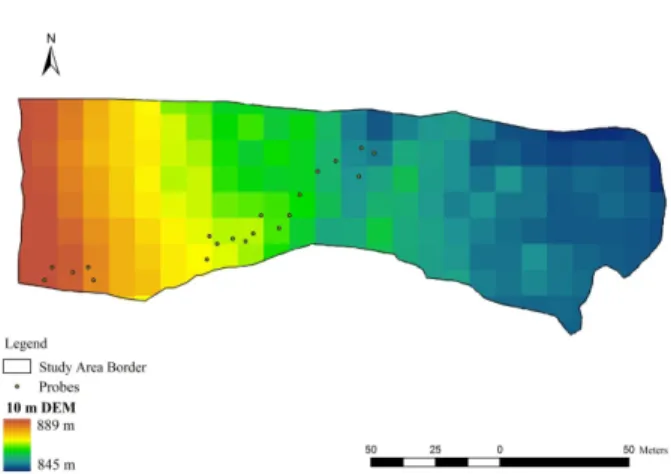
The DEMs quality is related to the degree of detail in which they can represent the topography. Thus, by calculating the correlations presented in Tables 1 and 2, the best representation of the study area could be made by using the 10 m resolution DEM (Figure 2) because of the best correlations with field data at that resolution, using both the TWI as the SWI. This is corroborated by Florinsky and Kuryakova (2000), who proposed the use of
According to the results presented in tables 1 and 2, from the evaluated wetness indexes, TWI showed the highest correlation with the moisture data measured in the field, being indicated as the most suitable for the representation of soil moisture in the study area. The SWI, although allowing the adjustment of multi to unidirectional flow (Menezes, 2011), was less effective to represent the soil moisture in the area due to less accurate adjustments in obtaining the modified contribution area taken into account during this index calculation.
Figure 3 shows the maps generated based on TWI and SWI methods for the 10 m resolution. It is observed that there are remarkable differences between the maps, which is explained by the fact that they were obtained by different calculation methods (Beven; Kirkby, 1979; Böhner et al., 2002; Böhner; Conrad, 2009). The SWI representation shows a continuing increase in the index value as the altitude decreases along the soil toposequence, showing greater similarity to the MDE (Figure 2). On the other hand, the TWI map represents an irregular behavior of the index values , but these values well correlated with the soil moisture data obtained by multisensor probe (Tables 1 and 2).
Regarding the wetness index values obtained by different resolution DEMs at the soil moisture measurement locals, it was noted that the coarser the maps resolution (larger cells), the higher the wetness indexes obtained (Figures 4A and 4B). In figure 4A, it can be seen that, for a given probe, the wetness index values, particularly the SWI, increase with coarsening of the resolution. This fact was also observed by Zhang and Montgomery (1994) and Wolock and Price (1994) who suggest that more detailed terrain features present in DEMs with smaller cells (better resolution) are
not well represented in larger cells DEM due to the progressive loss of resolution for both the drainage network and for sloping places, resulting in higher values in each cell.
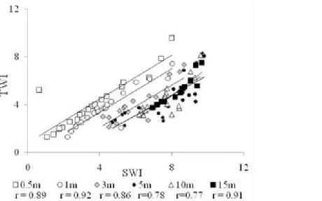
It is observed that the behavior of the wetness index values in relation to the resolution varies with the method of obtaining the index, being the SWI the one that showed marked index increase along with the coarsening of the resolution, which was not observed for the TWI method, which presented a much more discrete variation (Figure 4B). However, there were significant and positive correlations between the TWI and SWI obtained at different resolutions (Figure 5). There was no clear trend of increasing correlation between the indices with improved resolution, since in the coarsest resolution (15 m) it was found highly significant and positive correlation (R = 0.91 and p <0.001), which was also checked out for the second best resolution, 1 m, R = 0.92 and p <0.001 (Figure 5).
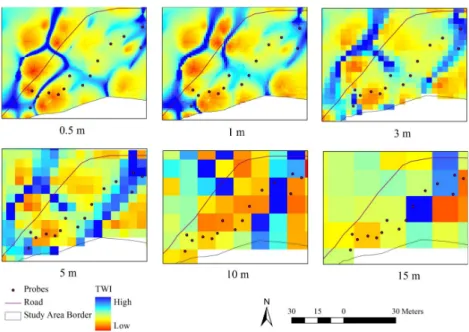
According to Thompson; Bell; Butler (2001), for a given MDE to represent well the soil-landscape relationships and soil properties variability in a continuous manner, it has to relate quantitatively and satisfactorily the environmental factors, such as topography, and soil properties, and also enable spatial predictions about soil properties to all over the study area, including those locations which were sampled. In this sense, the optimal DEM cell size is crucial and can be obtained by mathematical formulations (Hengl, 2006) or heuristically, being one of these estimated by the ratio between the area of interest and the double of the total perimeter (Sharma; Tiwari; Bhadoria, 2011). By this heuristic formulation, the appropriate grid size for the study area would be approximately 12 m (16,000 m² / [2x652 m]), which is very close to the 10 m resolution, corroborating with the best correlations obtained for this spatial resolution. For the visualization of the loss in details as the resolution decreases, just for illustration effect, in figure 6 are presented maps generated by the method TWI with different resolutions.
It is important to highlight, after exposing the data here obtained, that this kind of information can assist in hydrological and pedological studies, allow inferences about soil water content in the landscape, help decision makers about the use and management of soils in the area, and also provide more confidence in choosing the most appropriate places to grow different plant species, according to their adaptation to varying soil moisture conditions.
Figure 3 – TWI and SWI derived from the 10 m resolution DEM.
Figure 4 – Increasing wetness index values with increasing cell size. SWI values for each moisture sampling point with the probe, obtained at different resolutions DEM (A). TWI and SWI average values obtained from different resolutions DEMs (B).
Figure 6 – TWI maps obtained from different resolution DEMs.
CONCLUSIONS
The evaluated wetness indexes, TWI and SWI, showed significant and high correlation with soil moisture measured in the field at 100 cm depth, confirming the potential use of these indexes for supporting hydrological studies and soil use and management, especially for perennial plants with deep root systems.
The TWI at 10 m resolution was more closely correlated with soil moisture measured in the field.
The dry season showed better correlation between the wetness indexes with soil moisture determined in the field.
REFERENCES
BEVEN, K.J.; KIRKBY, M.J. A physically based, variable contributing area model of basin hydrology. Hydrological Science Bulletin, 24:43-69, 1979.
BEVEN, K.; WOOD, E.F. Catchment geomorphology and the dynamics of runoff contributing areas. Journal of Hydrology, 65(1):139-158, 1983.
BÖHNER, J.; CONRAD, O. System for Automated
Geoscientific Analyses (SAGA) 2.0.5. Available in: <http://sourceforge.net/projects/saga-gis/files/>. Accessed on: Feb. 20th, 2012. 2009.
BÖHNER, J. et al. Soil Regionalisation by means of terrain analysis and process parameterisation. In: MICHELI, E.; NACHTERGAELE, F.;
MONTANARELLA, L. (Eds): Soil Classification 2001. Joint Research Centre, Ispra, p.213-222, 2002.
EMPRESA BRASILEIRA DE PESQUISA
AGROPECUÁRIA – EMBRAPA. Sistema Brasileiro
de Classificação de Solos. 3.ed. Rio de Janeiro, 2013. 353 p.
FLORINSKY, I.V.; KURYAKOVA, G.A. Determination of grid size for digital terrain modelling in landscape investigations – Exemplified by soil moisture distribution at a micro-scale. International Journal of Geographical Information Science, 14(8):15-832, 2000.
GHIBERTO, P.J. et al. Components of the water balance in soil with sugarcane crops. Agricultural Water Management, 102(1):1-7, 2011.
GRABS, T. et al. Modeling spatial patterns of saturated areas: A comparison of the topographic wetness index and a dynamic distributed model. Journal of Hydrology, 373:15-23, 2009.
HU, W. et al. Watershed scale temporal stability of soil water content. Geoderma, 158(3-4):181-198, 2010. LAGACHERIE, P.; MCBRATNEY, A.B. Spatial soil information systems and spatial soil inference systems: perspectives for digital soil mapping. In: LAGACHERIE, P.; MCBRATNEY, A.B.; VOLTZ, M. (Eds). Digital soil mapping: an introductory
perspective. Amsterdam: Elsevier, v.1, p.3-24, 2007.
MCBRATNEY, A.B.; MENDONÇA-SANTOS, M. DE L.; MINASNY, B. On digital soil mapping. Geoderma, 117:3-52, 2003.
MENEZES, M. D. Levantamento pedológico
de hortos florestais e mapeamento digital de atributos físicos do solo para estudos hidrológicos. 2011. Available at: <http://bdtd.ufla.br/tde_busca/ processaPesquisa.php?processar=Processar>. Accessed on: Jun. 20th, 2013.
PETERS, P.H.C.R. et al. Acurácia e calibração de sonda de capacitância em Argissolo Vermelho-Amarelo. 2013. Available at:<http://www.cbcs2013.com.br/anais/ arquivos/2609.pdf>. Accessed on: Sep. 10th 2013.
PILESJÖ, P.; PERSSON, A.; HARRIE, L. Digital elevation data for estimation of potential wetness in ridged fields-Comparison of two different methods. Agricultural Water Management, 79:225-247, 2006.
PINHEIRO, H.S.K. et al. Modelos de elevação para obtenção de atributos topográficos utilizados em mapeamento digital de solos. Pesquisa Agropecuária Brasileira, 47(9):1384-1394, 2012.
REICHARDT, K.; TIMM, L.C. Solo, planta e
atmosfera: conceitos, processos e aplicações. Barueri: Manole, 2012. 524p.
SERAFIM, M.E. et al. Disponibilidade hídrica e distinção de ambientes para cultivo de cafeeiros. Revista Brasileira de Engenharia Agrícola e Ambiental, 17(4):362–370, 2013.
SHARMA, A.; TIWARI, K.N.; BHADORIA, P.B.S. Determining the optimum cell size of digital elevation model for hydrologic application. Journal of Earth System Science, 120(4):573–582, 2011.
STEIN, A.; RILEY, J.; HALBERG, N. Issues of scale for environmental indicators. Agriculture, Ecosystems & Environment, 87(2):215–232, 2001
SUMFLETH, K.; DUTTMANN, R. Prediction of soil property distribution in paddy soil landscape using terrain data and satellite information as indicators. Ecological Indicators, 8(5):485-501, 2008.
THOMPSON, J.; BELL, J.; BUTLER, C. Digital elevation model resolution: effects on terrain attribute calculation and quantitative soil-landscape modeling. Geoderma, 100:67–89, 2001.
WEIHUA, Z.; MONTGOMERY, D. Digital elevation model grid size, landscape representation, and hydrologic simulations. Water Resources Research, 30(4):1019–1028, 1994.
WILSON, J.P.; REPETTO, P.L.; SNYDER, R.D. Effect of data source, grid resolution and flow-routing method on computed topographic attributes. In: WILSON J.P.; GALLANT J.C. (Eds). Terrain Analysis: Principles and Applications. John Wiley & Sons: New York: p.133–161, 2000.
WOLOCK, D.M.; PRICE, C.V. Effects of digital elevation model map scale and data resolution on a topography based watershed model. Water Resources Research, 30:3041–3052, 1994.
ZHANG, W.; MONTGOMERY, D.R. Digital elevation model grid size, landscape representation, and
hydrological simulations. Water Resources Research, 30:1019–1028, 1994.