LoRaWAN Performance evaluation

Tiago Afonso Antunes de Figueiredo

LoRaWAN

Performance evaluation

Dissertação para obtenção do Grau de Mestre em Engenharia Eletrotécnica e de Computadores

Orientador: Luis Bernardo, Professor Associado com agregação, Universidade Nova de Lisboa

Júri

Presidente: Doutor João Carlos da Palma Goes - FCT/UNL

Arguentes: Doutor Luís Filipe Lourenço Bernardo - FCT/UNL (Orientador) Doutor Rodolfo Alexandre Duarte Oliveira - FCT/UNL (Arguente)

LoRaWAN Performance evaluation

Copyright © Tiago Afonso Antunes de Figueiredo, Faculty of Sciences and Technology, NOVA University Lisbon.

The Faculty of Sciences and Technology and the NOVA University Lisbon have the right, perpetual and without geographical boundaries, to file and publish this dissertation through printed copies reproduced on paper or on digital form, or by any other means known or that may be invented, and to disseminate through scientific repositories and admit its copying and distribution for non-commercial, educational or research purposes, as long as credit is given to the author and editor.

Ac k n o w l e d g e m e n t s

Ao meu orientador, que me motivou a fazer o melhor.

E aos meus amigos e família, com quem sempre pude contar.

Agradeço o apoio financeiro dado pela FCT/MCTES através de fundos nacionais e quando aplicável cofinanciado pelo FEDER, no âmbito do Acordo de Parceria PT2020 no âmbito dos projetos UID/EEA/50008/2019 e CoShare (LISBOA-01-0145-FEDER-0307095 - PTDC/EEI-TEL/30709/2017).

A b s t r a c t

The Internet of Things (IoT) is expected to grow in the upcoming years. LoRaWAN is one promising Low Power Wide Area Network (LPWAN) standard proposed for IoT widely adopted across the world. It runs on unlicensed spectrum and was designed to carry sporadic traffic.

This dissertation analyses the performance of LoRaWAN in extreme conditions, where peak traffic loads occur in the network. It starts by evaluating the Network Simulator 3 ( ns-3) LoRaWAN module, identifying and correcting their implementation. In a second phase, it evaluates the limitations of the class A LoRaWAN access protocol during synchronized peaks of traffic, and proposes a new access algorithm to improve the reliability and reduce the latency.

R e s u m o

É esperado que a Internet of Things (IoT) cresça nos próximos anos. O LoRaWAN é um standard Low Power Wide Area Network (LPWAN) proposto para IoT, adotado em todo o mundo. Este usa espetro não licenciado e foi desenhado para transmitir tráfego esporádico.

Esta dissertação analisa o desempenho da tecnologia LoRaWAN em condições extre-mas, quando picos de tráfego ocorrem na rede. A dissertação começa por primeiro avaliar a implementação de LoRaWAN no simulador Network Simulator 3 (ns-3), identificando e corrigindo a sua implementação. Numa segunda fase, esta avalia as limitações da classe A do protocolo de acesso LoRaWAN durante picos de tráfego sincronizado, e é proposto um novo algoritmo de acesso para melhorar a fiabilidade e reduzir a latência.

C o n t e n t s

List of Figures xiii

List of Tables xv Acronyms xvii 1 Introduction 1 1.1 Motivation . . . 1 1.2 Objectives . . . 3 2 Related Work 5 2.1 Introduction . . . 5 2.2 LoRaWAN . . . 5 2.2.1 Introduction . . . 5 2.2.2 Types of classes . . . 7 2.2.3 Specifications . . . 8 2.2.4 Deployment . . . 10 2.3 Alternatives to LoRaWAN . . . 10 2.3.1 802.11ah . . . 10 2.3.2 Sigfox . . . 12 2.3.3 Weightless . . . 12 2.3.4 RPMA . . . 13 2.3.5 NB-IoT . . . 13 2.3.6 Summary . . . 15 2.4 Simulators . . . 16 2.4.1 Introduction . . . 16 2.4.2 ns-3 . . . 17 2.4.3 OMNeT++ . . . 17 2.4.4 Summary . . . 18 3 Performance Evaluation 19 3.1 Evaluating the simulator . . . 19

C O N T E N T S

3.1.2 Problems with the simulator logic. . . 19

3.1.3 Modifications to the simulator . . . 20

3.2 Simulations. . . 22

3.2.1 Introduction . . . 22

3.2.2 Starting parameters . . . 22

3.2.3 Jitter tests - using additive random jitter to optimize throughput . 23 3.2.4 Variable jitter algorithm . . . 26

3.2.5 Jitter attribution algorithm. . . 27

3.3 Results . . . 28

3.3.1 Introduction . . . 28

3.3.2 Jitter test results . . . 28

3.3.3 Variable jitter algorithm results . . . 31

3.3.4 Jitter attribution algorithm results . . . 35

3.4 Comments and observations . . . 40

4 Conclusions and future work 41 4.1 Future Developments . . . 42

Bibliography 43

L i s t o f F i g u r e s

1.1 Comparison between different technologies. . . 3

2.1 LoRaWANs protocol Stack[4]. . . 6

2.2 LoRaWAN protocol Stack[1]. . . 7

2.3 A visual representation of how different classes transmit in LoRa. . . 8

2.4 Uplink timing diagram for confirmed data messages. . . 9

2.5 Belgium LoRaWAN coverage in 2016. . . 10

2.6 Example of NB-IoT operation mode[2]. . . 14

2.7 Example of message flow for RACH[2]. . . 15

3.1 Optimal maximum jitter fit curves with 95% confidence interval. . . 28

3.2 Unreliable throughput with an SF of 7 in function of the maximum jitter. . . 29

3.3 Reliable throughput with an SF of 7 in function of the maximum jitter. . . . 30

3.4 Unreliable throughput with an SF of 12 in function of the maximum jitter. . 30

3.5 Reliable throughput with an SF of 12 in function of the maximum jitter. . . . 31

3.6 Unreliable throughput with an SF of 7 with the variable jitter algorithm. . . 32

3.7 Reliable throughput with an SF of 7 with the variable jitter algorithm. . . 32

3.8 Unreliable throughput with an SF of 12 with the variable jitter algorithm. . . 33

3.9 Reliable throughput with an SF of 12 with the variable jitter algorithm. . . . 34

3.10 Delay with an SF of 7 with the variable jitter algorithm. . . 34

3.11 Delay with an SF of 12 with the variable jitter algorithm.. . . 35

3.12 Unreliable throughput with an SF of 7 with the jitter attribution algorithm. . 36

3.13 Reliable throughput with an SF of 7 with the jitter attribution algorithm. . . 37

3.14 Unreliable throughput with an SF of 12 with the jitter attribution algorithm. 37 3.15 Reliable throughput with an SF of 12 with the jitter attribution algorithm. . 38

3.16 Side by side comparison of the delay differences between the jitter attribution algorithm with an SF of 7 while converging and after the ideal state has been reached.. . . 39

3.17 Side by side comparison of the delay differences between the jitter attribution algorithm with an SF of 7 while converging and after the ideal state has been reached.. . . 39

L i s t o f Ta b l e s

2.1 Overview of different technologies . . . 16

3.1 Statistics of one transmission over a 10 minute period of the original code. . 21

3.2 Statistics of one transmission over a 10 minute period while transmitting an ACK on the second receive slot with changes to the SF attribution function and with the SF set based on distance. . . 21

3.3 Statistics of one transmission over a 10 minute period of the code modified transmit an ACK on the second receive slot. . . 21

3.4 Duration of a complete transmission according to SF . . . 22

3.5 Maximum jitter values for SF 7 in seconds. . . 25

Ac r o n y m s

3GPP 3rdGeneration Partnership Program.

ACK Acknowledgment.

AID Association Identifier.

AP Access Point.

BLE Bluetooth Low Energy.

CDF Cumulative Distribution Function. CoAP Constrained Application Protocol. CRC Cyclic redundancy check.

CSS Chirp Spread Spectrum.

DSSS Direct Sequence Spread Spectrum.

E-UTRAN Evolved Universal Terrestrial Radio Access Network. GPRS General Packet Radio Service.

GSM Global System for Mobile communications. GUI Graphical User Interface.

HTTP Hypertext Transfer Protocol.

IEEE Institute of Electrical and Electronics Engineers. IoT Internet of Things.

IP Internet Protocol.

ISM Industrial, Scientific and Medical radio bands. LPWAN Low Power Wide Area Network.

AC R O N Y M S

LTE Long Term Evolution. MAC Medium Access Control.

MQTT Message Queue Telemetry Transport. NB-IoT Narrow Band - IoT.

ns-3 Network Simulator 3. PHY Physical Layer. QoS Quality of Service.

QPSK Quadrature Phase-Shift Keying. RACH Random Access Channel. REST REpresentational State Transfer. RPMA Random Phase Multiple Access. SF Spreading Factor.

TCP Transmission Control Protocol. TIM Traffic indication map.

ToA Time on Air.

UDP User Datagram Protocol. WAN Wide Area Network.

C

h

a

p

t

e

r

1

I n t r o d u c t i o n

1.1

Motivation

Internet of Things (Internet of Things (IoT)) is the technology that connects any device to the Internet[1], being it a wearable, a car, or even a fridge. It is also used for sensors that can help industries, such as the oil industry, or in a city with smart meters, intelligent traffic management, air quality control, and more. These devices allows us to have a vast amount of information, relatively cheaply, and with a great impact in our lives. They are expected to grow in number, with an estimation of over 25 billion devices by 2020 [2].

IoTdevices possess several requirements that need to be fulfilled, such as a low price and the need for low energy consumption. In order to meet these requirements, not only do the devices have basic processors that are power efficient, but also rely on transmission protocols that are themselves power efficient. IoT networks may span over a wide area, over different environments. Therefore, a protocol is needed that not only can cover a wide area, but is also scalable, in order to support an increasing number of devices. For example, a city may want to have an intelligent traffic management system that reacts in real time to the current traffic conditions, or the ability to know when certain garbage cans are full to make their pickup more efficient. IoT can also be privately used, for instance, in smart home applications. These applications do not often need to send high volumes of data, with the norm being infrequent and small data packages. Although throughput is not one of the biggest needs in IoT, reliable transmission is a must for a subset of the applications, for instance in security surveillance.

Despite the fact that wired options are available for connectivity, wireless is preferred since it offers more flexibility. There are several different technologies in this field, includ-ing ZigBee, Bluetooth (in particular, Bluetooth Low Energy (BLE)), Wi-Fi, 3rd Generation Partnership Program (3GPP) mobile networks(2G/3G/4G) and LPWANs.

C H A P T E R 1 . I N T R O D U C T I O N

The first technologies described, Wi-Fi, BLE and ZigBee, work on a short range. They are all based on the 2.4 GHz frequency (as well as 5 GHz for Wi-Fi) and optionally the 868/915 MHz unlicensed frequency bands for ZigBee [3], and they all have a range of around 100/150 m on an unobstructed line of sight. Between the three of them, Wi-Fi is used when there is the need for higher data rates. BLE and ZigBee are similar, with the later having a longer range because it may use a mesh network. In a mesh network, the nodes are capable of receiving and transmitting packages from neighbour nodes, increasing the coverage and reliability of the network, since several nodes need to fail in order for one to become isolated. The limitations of this technology are the higher communication delays derived from multihopping and the non-negligible control traffic required to maintain the network. Combined with a non uniform network topology, this leads to an uneven battery consumption throughout the network[3]. Despite the fact that most homes these days have a widespread adoption of Wi-Fi and Bluetooth, as well as with ZigBee networks already in use, like in Philips Hue products, the main gripe with these technologies is the short range and the high number of devices that can cause severe interference.

At larger ranges, we have two main choices: 3GPP mobile networks (2G/3G/4G) and LPWANs. The former currently have a big widespread coverage, to the point where most countries already have an almost full coverage nationwide, or at least where human population resides or traverses. Although 2G and 3G don’t offer high throughputs, 4G improves on this, while at the same time offering Quality of Service (QoS), but as a trade off, mobile networks can be extremely expensive while also having a high power demand and supporting a low maximum number of devices per base station. 3G and 4G networks without any changes will have issues with a large network of IoT devices, since they are not prepared to handle lots of nodes at the same time making them not ideal. 4G Narrow Band - IoT (NB-IoT) is the best 3GPP alternative to LPWANs, with similar energy efficiency, higher throughput and offering better QoS. LPWANs offer a high coverage area per gateway, while supporting a very large number of devices (many thousands), with a reduced power and monetary cost, with the trade off being the slower data rates.

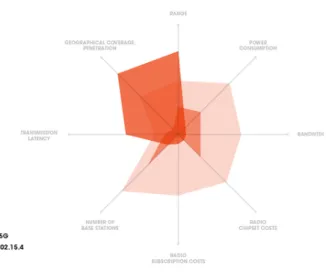
Figure1.1depicts the ups and downs of some of these technologies, showing that the LPWANs are strong in the fields of geographical coverage, range, power consumption and costs, while lacking in bandwidth and transmission latency. ZigBee has higher band-width, no radio subscription costs and lower latency, but lacks in every other department compared to LPWANs. 3GPP mobile networks, on the other hand, are an in between of both previous technologies in range, geographical coverage and latency, but have a much higher bandwidth at the cost of higher overall monetary costs and power consumption.

The discussed solutions meet some of these requirements for IoT devices. This disser-tation focuses on LoRaWAN, one of the most promising standards at the time of writing.

1 . 2 . O B J E C T I V E S

Figure 1.1: Comparison between different technologies.

1.2

Objectives

The main goal of this dissertation is to explore how LoRaWAN performs in a scenario of peak traffic loads, as in the example of an earthquake. We intend to study how the protocol handles correlated peaks of load, and what impact it will have for the individual users of the network. We will test how uncontrolled user transmissions affect the overall reliability, and propose a new algorithm in the Medium Access Control (MAC) layer that serves the purpose of improving the throughput and reliability of transmissions across the network.

The dissertation is organized starting with the state of the art on chapter 2, where an overview of existing technologies and competing protocols is given, finishing by show-ing different simulators that can be used to simulate a LoRa network. After, chapter 3 presents the work done in the simulator. It starts with an evaluation of the accuracy of the simulator to model the MAC and Physical (PHY) layers, fixing any encountered issues. This is followed by the proposal of new access protocols with the objective of improving the reliability, and their performance evaluation. The dissertation ends with chapter 4, where after the final conclusions, other directions are discussed for this topic.

C

h

a

p

t

e

r

2

R e l a t e d Wo r k

2.1

Introduction

Chapter 2 reviews the existing literature about LoRaWAN, exploring how it works and how it performs. It also presents competing technologies, comparing them. The chapter ends with an overview of existing simulation environments for LoRaWAN.

2.2

LoRaWAN

2.2.1 Introduction

LoRaWAN is a LPWAN developed by Cycleo (a French company acquired by Semtech) and is intended for wireless battery-operated devices, which can be used in the deployment of IoT. It targets bi-directional communications, mobility and localization services. It provides seamless interoperability without the need of complex local installations. This technology is usually installed in a star-of-stars topology, where the gateways act as a transparent bridge carrying messages between end devices and the network server. Gate-ways are connected to the network via standard IP connections, while the end devices are connected via single-hop wireless communication to one or more gateways. Figure2.1

C H A P T E R 2 . R E L AT E D WO R K

Figure 2.1: LoRaWANs protocol Stack[4].

At the most basic level, a LoRaWAN network is constituted by end-devices, also known as the clients, and by gateways. The end-devices collect and/or receive informa-tion and are connected to one or more gateways, which are also known as base stainforma-tions, through the LoRaWAN radio layer. Beyond this point, the gateways will connect to the network server through IP connectivity. The server is the center of the star topology. There is an application layer that describes the code running on the end-device and behind the network server. This layer can be connected to the server with different connection tech-nologies, as seen in figure2.2, such as Constrained Application Protocol (CoAP), Message Queue Telemetry Transport (MQTT), among others[5].

• CoAP is an application layer protocol for IoT applications. It defines a web

trans-fer protocol based on REpresentational State Transtrans-fer (REST) on top of Hypertext Transfer Protocol (HTTP) functionalities. CoAP uses User Datagram Protocol (UDP) communication by default, more suited for IoT applications since this protocol is relatively simple. It is built in two layers, the messaging, which detects duplica-tions and offers reliable communication over UDP (which has no error recovery mechanism), and the request/response sublayer that handles REST communica-tions. CoAP also utilizes four types of messages, confirmable, non-confirmable, reset and acknowledgment, with reliability being achieved with a mix of the first two. Some important features of this protocol include on-demand subscriptions to monitor resources of interest using a publish/subscribe mechanism, the ability to interact with HTTP, due to the common REST architecture that enables CoAP to interact with HTTP using a proxy and security[1].

• MQTT is another application layer protocol. It uses a publish/subscribe pattern

where devices publishes their information to a broker, and the subscriber gets the desired data from it. MQTT is built over the Transmission Control Protocol (TCP)

2 . 2 . L O R AWA N

protocol, supporting three QoS levels, and with two major specifications, MQTTv3.1 and MQTT-SN. MQTT-SN was defined specifically for sensor networks, defining a UDP mapping of MQTT and adding broker support for indexing topic names. In MQTT-SN the device publishes a topic to the broker, with certain information, that is forwarded to the subscribers, which subscribed to related topics and are waiting to be informed by the broker. When new data is generated, the device sends it to all subscribers through the broker, with the last one providing security by checking the authorization of the publisher and the subscriber. On the message payload, a retain field informs the server whether the last published message is to be saved and sent to any new subscribers as the first message, or not. This protocol is already being used by some applications, like Facebook notifications[1].

Figure 2.2: LoRaWAN protocol Stack[1].

2.2.2 Types of classes

There are 3 types of classes for LoRaWAN communications, although, it is required that all devices can work as class A. The following classes exist:

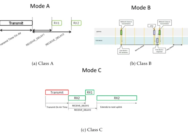
A Bi-directional end-device (class A), illustrated in figure 2.3a, is used by the lowest power end-devices. Class A devices are not actively listening to the server, and will only receive frames after an uplink transmission. This class has the highest latency. It works by having two short downlinks receive windows after making a transmission. The transmission slot schedule is based on the end-device’s own communication needs with a small time-based variation (ALOHA type).

C H A P T E R 2 . R E L AT E D WO R K

B Bi-directional end-device with scheduled receive slots (class B) are like class A, but they

possess a receive window at scheduled times. For the end-device to open its receive window, it receives periodic time synchronized beacons from the gateway and this allows the server to know when the device is listening. The class B access mode is shown in figure2.3b.

C Bi-directional end-device with maximal receive slots (class C), shown in figure2.3c, is usually used by devices connected to a permanent energy source, having the lowest latency. It has a nearly continuously open receive windows that are only closed when the device is transmitting.

(a) Class A (b) Class B

(c) Class C

Figure 2.3: A visual representation of how different classes transmit in LoRa.

2.2.3 Specifications

LoRaWAN is a semi-proprietary standard, with the specifications open, but with the chipsets for the end-device only being sold by Semtech. This makes the base stations relatively cheap, but the end-device may be more expensive than other alternatives. As discussed before, it has several classes that provide the standard versatility and appli-cability for different situations. In Europe, it uses a bandwidth of 125 or 250 KHz, and supports data rates from 250 bps to 50 Kbps, depending on the spreading factor, using the frequencies 433/868/780/915 MHz Industrial, Scientific and Medical (ISM). The fact that only one chipset vendor exists harms this technology, since availability can be

2 . 2 . L O R AWA N

limited, potentially making users migrate to competing technologies. It possesses a range of 2-5 km in urban areas and up to 15 km in suburban areas[6], while having a transmit power of 14 dBm in Europe and 27 dBm on the US. Version 1.1 of the standard intro-duces features to support roaming and defines a specification for geo-location parameters. The bidirectional communication is provided by a special Chirp Spread Spectrum (CSS), which spreads the narrow band input signal over a wider bandwidth, resulting in a signal harder to detect and jam, and more resistant to effects such as multipath, fading and Doppler effect[7]. LoRaWAN supports spreading factors (SF) between 7 and 12, which trades-off range for data rate, with the SF value of 7 having the shortest range and highest data rate, and an SF of 12 having the largest range but with the lowest data rate[8]. The SF value is attributed when a new node connects to the base station. The packet size is defined by the user and can be between 51 and 222 bytes, depending on the SF used. Since the SF symbols are orthogonal, the same gateway can receive different transmissions with different SFs simultaneously, although in real life scenarios, this might not always be the case[9]. In Europe, 3 bands are used for transmission, each with different duty cycle

limitations of 0.1%, 1% and 10%. The band at 868 MHz has a 1% duty cycle and in the main band used for transmissions carrying 3 channels. When a node wants to transmit, it chooses one of these channels pseudo-randomly before starting the transmission. Lo-RaWAN also supports reliable traffic, with the base station sending an Acknowledgement (ACK) frame to the node when it receives a successfully transmission. Two ACK frames are transmitted in two receive windows. The second window is opened one second after the first one. The first ACK is sent on the same channel and with the same SF as the received transmission; the second ACK is sent on the dedicated ACK channel with a duty cycle of 10% with an SF of 12, during the node’s second receive window. If the node receives the ACK on the first window, it will not open the second one. Otherwise, if a node receives neither ACK frame, it retransmits the previous data until a successful ACK reception occurs, as is depicted in figure2.4.

C H A P T E R 2 . R E L AT E D WO R K

2.2.4 Deployment

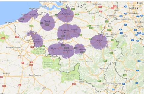
LoRaWAN has seen an increasingly high deployment[10], with several countries deploy-ing the technology, as the example of Belgium (see figure2.5).

Figure 2.5: Belgium LoRaWAN coverage in 2016.

As of August of 2018, there are 49 countries with LoRaWAN coverage through telecom-munication companies, and 95 countries with LoRaWAN deployments [11]. Most of these deployments are thanks to "The Things Network"[12], a community driven network, where individuals may create there own network, expanding the coverage of LoRaWAN to areas that would not otherwise have it. It is also possible for private or public entities to create their own network. For example, a city creating a smart city.

2.3

Alternatives to LoRaWAN

There are several competing technologies in the Wide Area Network (WAN) space for IoT communication. This section takes a look at each of them, with their own individual advantages and disadvantages.

2.3.1 802.11ah

The first technology discussed is 802.11ah[13], also known as HaLow. It was published in 2017 by the Institute of Electrical and Electronics Engineers (IEEE) as a competing standard in the WAN world. It is one of the most recent of all the IoT standards, a reason why currently no devices that uses this technology can be found at the time of writing. It has a variable data rate that can go up to 347 Mbps, allowing a packet size of up to 7991 bytes without aggregation, and 65535 bytes with aggregation and with a range of up to 1 Km while its transmit power is located between 1 mW and 1 W. HaLow

2 . 3 . A LT E R N AT I V E S T O L O R AWA N

spectrum offers 26 MHz of bandwidth, using different types of modulations and coding options according to the desired data rate, while using license exempt bands bellow 1 GHz, excluding the TV white space. It also supports 8191 network stations, with one being a relay access point with the task of helping other stations passing along messages over long distances. This technology does not allow for end node roaming, requiring other IEEE 802.11 amendments to do so. 802.11ah stations are grouped into one of three types:

• Traffic indication map (TIM) stations are the only ones that needs to be constantly

listening to the Access Point (AP) beacons to send or receive data, and said data must be transmitted within a restricted access window period, divided into differentiated segments for uplink, downlink and multicast. Stations that have high traffic load should use this type since it combines energy efficiency mechanisms and periodic data transmission.

• Non Tim stations do not need to listen to any beacon; during the association process,

these devices negotiate with the AP directly to receive a transmission time allocated in a periodic restricted access window. After this, the station can either request a new window, or keep the negotiated one.

• Unscheduled Stations are similar to Non Tim stations in the fact that they do not

need to listen to the beacon, but they can send a pool request to the AP asking for immediate access to the channel, even during restricted access windows. The response frame will indicate a frame outside any restricted access window where the unscheduled station can access the channel. This type is only used for stations that sporadically join the network.

The power mechanism that this standard employs on TIM stations in order to save power is to put the device to sleep by deactivating the radio module during non-traffic periods. Another way 802.11ah uses to increase sleep time and reduce station competition for a channel is the TIM information map restricting the stations allowed to access and the page segmentation. When a station joins a network, it is given an Association Identifier (AID) that defines which hierarchical group it belongs to. This makes it so that instead of all stations being able to compete at the same time, only stations of the same group can do it in a specific period, allowing all other stations to remain is sleep mode and reducing collisions. Some applications for this technology can be the agricultural automation, smart metering, industrial automation and animal monitoring, since these applications do not require massive amounts of devices or range, while at the same time needing a high packet delivery rate and low delay [13].

Another similar technology developed by IEEE is 802.11af, possessing a longer range of over 3 Km, and making use of unused TV channels from 54 to 698 MHz, with the base station queering a database to see what channels are available locally for data transmis-sion.

C H A P T E R 2 . R E L AT E D WO R K

2.3.2 Sigfox

Sigfox[14] is at the time of writing one of, if not, the biggest IoT networks in the world with, as of late 2017, coverage of 36 countries, 17 of them nation wide. It is a proprietary standard developed by a company of the same name. The company makes the endpoint openly available, so it is relatively inexpensive for the consumer, but the base station is exclusively developed by them and deployed by an operator who pays the royalties. Sigfox uses 192 KHz of the publicly available band, in the 868 MHz and 902 MHz ISM frequencies, and with a relatively low data rate of 100 or 600 bps, depending on the region. The low data rate is adapted for small, infrequent burst of data. With a range of up to 50 Km, Sigfox can be deployed nationwide with a relatively low cost due to the low number of base stations needed and taking advantage of end node roaming. Due to regional regulations, a limited duty cycle 1% is imposed, only allowing a per day maximum of 140 uplink messages with 12 bytes each and 4 downlink messages of 8 bytes each[15]. The limitation of 4 download messages per day means that an ACK message for every uplink is not possible, leading to poor reliability assurance. To increase the reliability, it transmits the message multiple times (with a default of three messages using different frequencies). Sigfox also has a relatively low minimum power consumption, from 10 µW to 100 mW. This technology is good for applications that do not need frequent communications, like smart farming or smart buildings[16].

2.3.3 Weightless

Weightless is the only fully open standard[17] presented in this document, and because of this, the hardware cost is relatively low compared to the other standards. It was developed by Weightless SIG, a non profit organization, and this standard provides some interesting features, like firmware over the air. Similarly to LoRaWAN, this standard also defines different types of classes for different needs, making this technology more versatile. All three types have different characteristics that are more suited for certain uses, but all of them share a transmit power of 17 dBm, allow roaming and support an unlimited number of devices. The three classes are presented:

1. Weightless-P is the most recent technology, offering a bidirectional protocol with

QoS tiers. It has a 12.5 KHz channel on the sub-GHz frequency, with data rates from 200 bps to 100 Kbps, a packet size of 10 bytes minimum, and a range of up to 2 Km. It is ideal for private networks and cases where up and downlink traffic is required.

2. Weightless-N is a ultra-narrowband system, similar to Sigfox and LoRaWAN class A,

and it is more orientated towards sensor-based networks, having a range of up to 3 Km. It uses ultra narrow band, around 200 Hz with 100 bps uplink with a packet size of up to 20 bytes, but with no downlink. It is an option to consider above the

2 . 3 . A LT E R N AT I V E S T O L O R AWA N

other two, since being open source means it is not only cheaper, but its availability is greater.

3. Weightless-W uses the TV white space, with a 5 MHz channel width and a 5 Km

range, but compared to the other Weightless standards, it has a shorter battery life and the frequency in which it operates can vary from city to city. It is the least popular of the three. Due to the unused TV bands varying greatly between regions, this standard ends up having very limited used, leading to very limited commercial availability. Its packet size is the same as the -P variant, 10 byte minimum, but with a higher data rate of 1 Kbps to 10 Mbps.

Weightless uses Direct Sequence Spread Spectrum (DSSS) to extend the range and decrease the data rate as a trade-off. This works by multiplying each transmitted symbol by a code word, resulting in a longer effective bit duration or a higher transmitted data rate. Because of weightless lower costs compared to other specifications, it is useful for devices massively deployed that require lower costs and don’t necessarily need a big range, like smart home devices.[18].

2.3.4 RPMA

Random Phase Multiple Access (RPMA) is a proprietary standard developed by Ingenu[19], that uses the globally available, and unlicensed band of 2.4 GHz, which means there is no need to create different radio modules for different regions. It is a well established technology, already present in 29 countries world wide as of February 2017. It has a good maximum range of almost 13 Km, while also having high data rates, with a 1 MHz channel, 625 Kbps uplink and 156 Kbps downlink and a transmit power of up to 20 dBm. This allows for a lower number of base stations to cover a bigger area, while at the same time allowing a bigger data throughput. This technology also supports roaming and firmware over the air, vital to keep the devices future-proof. It supports packet sizes of 6 bytes to 10 KB, allowing for a wide range of information transmission. RPMA is a versatile technology, that supports high data rates, making it ideal for smart energy metering, allowing for high volumes of data to be transmitted in real time.

2.3.5 NB-IoT

NB-IoT is a technology developed by 3GPP and introduced as part of Release 13. Al-though not being fully backwards compatible, it is designed to co-exist with legacy Global System for Mobile communications (GSM), General Packet Radio Service (GPRS) and Long Term Evolution (LTE). This technology targets ultra-low-end IoT applications and uses existing available cellular spectrum. It has the highest gateway and end-device cost out of all other standards discussed, but also possesses some interesting features that differentiate it like QoS, roaming, low latency and the ability to integrate it with the already existing cellular networks with a software update, making it a really interesting

C H A P T E R 2 . R E L AT E D WO R K

alternative for countries or cities with well established cellular networks. To integrate in an existing network, a minimum of 180 KHz bandwidth is needed. The network operator can replace one GSM carrier (200 KHz), as well as inside an LTE carrier by allocating one of the Physical Resource Blocks of 180 KHz, as seen in figure2.6[20]. With this frequency band selection, the following operation modes are supported:

• Stand-alone operation when using one GSM frequency band.

• Guard-band operation when utilizing the unused resource blocks on the LTE carrier’s

guard band.

• In-band operation when utilizing the resource blocks within an LTE carrier.

The data rate is limited to 200 Kbps downlink and 20 Kbps uplink, with a 200 KHz bandwidth and with a packet size of 100 to 1000 bytes. As a trade-off for having lower latency than competing standards, it suffers from lower battery life, having a transmit power of 100 mW. The modulation used is Quadrature Phase-Shift Keying (QPSK), which will lead to a decreased resilience to interference. The protocol stack for NB-IoT is a reduced version of the protocol stack of LTE, with features such as handover, measure-ments to monitor the channel quality, carrier aggregation, and dual connectivity removed. NB-IoT can reuse the existing Evolved Universal Terrestrial Radio Access Network ( E-UTRAN) architecture and its backbone with minimal changes to it. This technology also benefits from using a licensed spectrum and having a time slotted synchronous protocol that uses the Random Access Channel (RACH) shown in figure2.7, leading to higher QoS than competing standards. Battery use is higher since it requires infrequent but regular synchronization. Since NB-IoT deployment is dependent on LTE and GSM infrastructure, it means that this technology may not be ideal for rural areas and zones that have poor or lack of LTE and GSM coverage. NB-IoT can be used in applications that require lower latency, higher QoS and higher data rates than the ones provided by technologies operat-ing in unlicensed spectrum. Like in retail, with point of sale terminals, or even alarms[2,

16,21].

Figure 2.6: Example of NB-IoT operation mode[2]. 14

2 . 3 . A LT E R N AT I V E S T O L O R AWA N

Figure 2.7: Example of message flow for RACH[2].

2.3.6 Summary

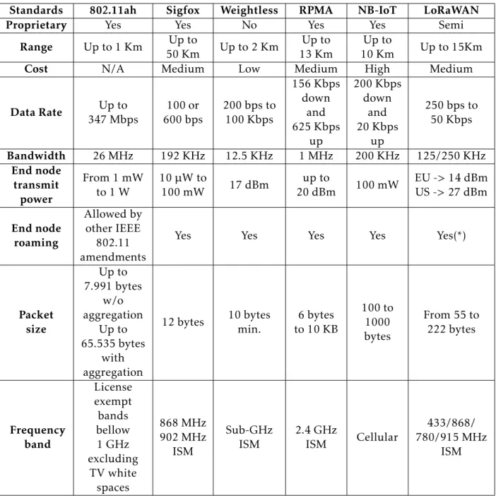
Table2.1provides a quick overview over the discussed technologies. The cost measure-ment is related to the base station, and end-device prices, with some technologies having the base station more expensive than others. All the bandwidth and data rate values are referring to the European frequencies. Most technologies have a coverage range between 10/20 Km, with Sigfox having the highest one, making it ideal for situation where a low amount of stations is preferred, and 802.11ah having the shortest at 1 Km, useful when range is not an issue. Most technologies support data rates in the order of Kbps, with Sigfox having the lowest with 100 or 600 bps, depending on the region, and 802.11ah having the highest with up to 347 Mbps, showing a trade-off between range and data rate. All technologies support roaming, with the exception of 802.11ah that needs other 802.11 amendments. The packet size varies between technologies, with Weightless not having a maximum, but having a minimum of 10 bytes, and Sigfox using a fixed size of 12 bytes per packet. 802.11ah has a maximum packet size dependent on if it has aggregation or not, and RPMA and NB-IoT have a range of packet sizes.

C H A P T E R 2 . R E L AT E D WO R K

Table 2.1: Overview of different technologies

Standards 802.11ah Sigfox Weightless RPMA NB-IoT LoRaWAN

Proprietary Yes Yes No Yes Yes Semi

Range Up to 1 Km Up to 50 Km Up to 2 Km Up to 13 Km Up to 10 Km Up to 15Km

Cost N/A Medium Low Medium High Medium

Data Rate Up to 347 Mbps 100 or 600 bps 200 bps to 100 Kbps 156 Kbps down and 625 Kbps up 200 Kbps down and 20 Kbps up 250 bps to 50 Kbps Bandwidth 26 MHz 192 KHz 12.5 KHz 1 MHz 200 KHz 125/250 KHz End node transmit power From 1 mW to 1 W 10 µW to 100 mW 17 dBm up to 20 dBm 100 mW EU -> 14 dBm US -> 27 dBm End node roaming Allowed by other IEEE 802.11 amendments

Yes Yes Yes Yes Yes(*)

Packet size Up to 7.991 bytes w/o aggregation Up to 65.535 bytes with aggregation 12 bytes 10 bytes min. 6 bytes to 10 KB 100 to 1000 bytes From 55 to 222 bytes Frequency band License exempt bands bellow 1 GHz excluding TV white spaces 868 MHz 902 MHz ISM Sub-GHz ISM 2.4 GHz ISM Cellular 433/868/ 780/915 MHz ISM

(*) Only on version 1.1 of the standard

2.4

Simulators

2.4.1 Introduction

There are several simulators that model certain characteristics of a LoRa network allowing the test of certain network configurations. Some of them are presented below.

2 . 4 . S I M U L AT O R S

2.4.2 ns-3

The first module tested was based on network simulator 3 (ns-3), an open source simu-lator that has no graphical user interface (GUI) and is based on the Linux terminal. Its installation is very easy, with the user only needing to extract a folder, and has a lot of documentation for the users. Out of the box, the module brings several examples, high-lighting a simple network test, which does a simple transmission from a node to a base station, and a complete network test, where the user can easily change the number of nodes, gateway rings, number of gateways and the radius. The simulation returns some useful statistics such as power to noise ratio, collisions, average time on air, and successful transmissions. This simulator also allows changes to the MAC layer, as well as the PHY layer and to the SF attribution algorithm. The PHY layer handles all the transmissions, calculating the time on air, path fading, and interference. At the time of writing, it only supports the European regional transmission parameters, although this can easily be modified[22].

2.4.3 OMNeT++ 2.4.3.1 Aloha based

On the OMNeT++ environment, the first module tested was Aloha based, with the files being extracted into the Aloha folder in the environment. This module is extremely limited compared to others, only modelling the physical and MAC layers. The user can choose several parameters like the number of hosts, their distance to the gateway, time slot, data rate. For different parameters the network can be overloaded, optimal or low traffic. In the end, the simulation returns statistics about collisions, time on air and lost packages. This simulator lacks the ability to control the nodes SF, signal power levels, packet retransmission from them and lacks the ACK messages from the gateway and any sort of MAC or physical layer tuning possibility. Unlike the ns-3 simulator, OMNeT++ offers a GUI, proving easier to use and configure[23].

2.4.3.2 FLoRa

Another OMNeT++ module offered is FLoRa[24]. This module is independent, allowing for easier end user changes. It requires specific versions of the OMNeT++ and the INET framework, with newer versions resulting in failed compilations. It comes with a pre existing scenario, where a network with 10 nodes, a network server and a gateway exist. The nodes are placed at random distances, and transmitting frames at random times, and the transmission power and spreading factor are also being generated randomly. At the end of the simulation, a file is generated with the statistics, that include power to noise ratio, percentage of collisions, average time on air, between others. It is possible to change the MAC and Physical layers, as well as the SF attribution.

C H A P T E R 2 . R E L AT E D WO R K

2.4.4 Summary

All the simulators studied, all explore LoRaWAN class A, but all provide different levels of flexibility, with ns-3 proving to be the most versatile. On the OMNet++ side, the Aloha based simulator is easy to use and offers some configurations for the user, but provides limited results. FLoRa provides similar results as the ns-3 simulator, but with a graphical interface for easier user interaction, but with less configurability than the ns-3 module.

C

h

a

p

t

e

r

3

P e r f o r m a n c e E va lua t i o n

3.1

Evaluating the simulator

3.1.1 Introduction

In order to study the LoRaWAN protocol, the version 3.28 of the ns-3 was used in con-junction with the LoRaWAN module explored in2.4.2. In a first phase, trials were made in order to properly evaluate the correct behaviour of the module.

3.1.2 Problems with the simulator logic

After starting the work with the simulator, we tested how the existing examples were being implemented, and how the simulator behave from the point of creating a node to how the transmissions were being implemented. For this we used the included examples called simple lorawan network example and complete lorawan example. We first started with only one node transmitting, and while we were testing the SF attribution, we noticed that at certain distances, the node would manage to have its packet received by the base station, but would not receive the corresponding ACK frame. This behaviour lead us to discover that the automatic SF attribution was not working reliably.

To test if interference was being correctly modelled, we prepared several tests where transmissions were synchronized to cause destructive interference (i.e. collisions) be-tween data frame transmissions, or bebe-tween data and ACK frames. During the tests with more than one node, more precisely having a packet from one node causing destructive interference with an ACK frame meant for another node, we noted that the second node would not receive an ACK frame on the second time slot, even if it was open. This showed that the network server was not being correctly implemented either. We also noticed that both the included periodic and one shot senders did not have any logic to provide reliable

C H A P T E R 3 . P E R F O R M A N C E E VA LUAT I O N

transmissions, nor was there a way for these classes to know if a node had received an ACK. Therefore, we identified the necessity to correct these errors and to implement a new kind of node, which implements reliable transmission of data.

3.1.3 Modifications to the simulator

In order to properly simulate a node behaviour, the issues encountered in3.1.2had to be fixed. The modifications implemented are described below, identifying the classes where they were made.

3.1.3.1 Node mac

On this class, a function was created in order to know if an ACK frame had or not been received by a node.

3.1.3.2 Network Server

The existing network server did not send ACK frames on both reception slots. So, we added code to schedule the transmission of a second ACK on the dedicated ACK channel, one second after the first transmission was done. This improved the ACK reception from the values showed in table3.1to the ones in table3.2.

3.1.3.3 SF attribution

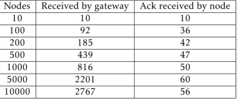
The existing code attributed the lowest possible SF that allowed for a successful reception by the gateway. This is done by using a default function on ns-3 that calculates the power a transmission has after a certain distance, in this case, between the node and the gateway. After this, the transmission power is checked against the sensitivity of the gateway, and the lowest SF is attributed according to the lowest power it can receive. This works well, since lower SF values have less time on air and therefore allow for higher data frame transmission rates to occur. After some testing, we found that the ACK sent by the gateway was not always received by the node due to the signal power being inferior to the sensitivity of the node. This happens because the nodes[25] usually have a lower sensitivity than the gateways[26]. Therefore, with the same transmission power, a packet may be received by the gateway, but not by the node. The code was changed to reflect this, checking the received power at the node instead of the gateway. Another function was added for manual SF definition. We can see in table3.3, that the number of transmissions received by the gateway is higher than the ones in table3.2. This is due to fact that lower SF values can be attributed, which leads to less time on air, and more transmissions being made.

3 . 1 . E VA LUAT I N G T H E S I M U L AT O R

Table 3.1: Statistics of one transmission over a 10 minute period of the original code. Nodes Received by gateway Ack received by node

10 10 8

100 93 5

200 176 5

500 428 5

1000 746 10

Table 3.2: Statistics of one transmission over a 10 minute period while transmitting an ACK on the second receive slot with changes to the SF attribution function and with the SF set based on distance.

Nodes Received by gateway Ack received by node

10 10 10 100 93 33 200 176 39 500 428 46 1000 746 50 5000 1825 63 10000 2222 63

Table 3.3: Statistics of one transmission over a 10 minute period of the code modified transmit an ACK on the second receive slot.

Nodes Received by gateway Ack received by node

10 10 10 100 92 36 200 185 42 500 439 47 1000 816 50 5000 2201 60 10000 2767 56

3.1.3.4 Reliable one shot sender

In order to have reliable transmission the class reliable one shot sender was created. It implements a single packet transmission where the sender checks if the corresponding ACK frame has been received. This is checked after the maximum period of time it takes to receive an ACK frame according to table3.4. These values were calculated by using the maximum payload size according to the LoRa standard. To calculate the time on air, we divide the payload size by the bitrate of the SF used. The reception time is calculated according to both reception slots, with the first opening 1 s after the transmission has ended, and the second slot, 1 s after the first slot. The reception slots duration is 0.2 s for each one. We only account for the duration of the second slot since it starts 1 s after the first slot started, and not after it finished. The time is the maximum time it can

C H A P T E R 3 . P E R F O R M A N C E E VA LUAT I O N

take from the beginning of a transmission, until the closure of the second ACK frame. If no ACK has been received during the maximum transmission time, the node makes a retransmission, waiting a random back off time. The back off time is picked from an uniform distribution, ranging from 0 s to the double of the maximum transmission time. After 3 failed attempts, the node will drop that transmission.

Table 3.4: Duration of a complete transmission according to SF

SF 7 8 9 10 11 12

Max payload (bytes) 222 222 115 51 51 51

Bitrate (byte/s) 683,75 394 220 122,5 55 31,25 Time (s) 0,325 0,563 0,523 0,416 0,927 1,632

Reception Time (s) 2 2 2 2 2 2

Reception slot duration (s) 0,2 0,2 0,2 0,2 0,2 0,2 Total reception time (s) 2,2 2,2 2,2 2,2 2,2 2,2 Max transmission time (s) 2,525 2,763 2,723 2,616 3,127 3,832

3.1.3.5 Reliable periodic sender

The reliable periodic sender is similar to the already existing periodic sender, but with some added logic implemented. This new class allows for different starting conditions, such as all nodes starting a transmission at the same time, or starting a transmission according to a Poison distribution. It also makes possible to change the minimum period according to the node’s SF, and allows for several different packet sending mechanics, that will be explored in section3.2.

3.2

Simulations

3.2.1 Introduction

A variable number of clients exists in a LoRa network. These clients usually send packets periodically but during certain situations, for instance, during a natural disaster, they may create load peaks of traffic on the network, leading to an increased number of packet collisions.

On this section we study how a network behaves during these load peaks, where reliability is a must, and how to improve it while at the same time understanding the drawbacks of high reliability. We first simulate how jitter affects periodic transmissions, and then present two algorithms developed on the MAC layer to control the jitter. 3.2.2 Starting parameters

Our simulations have as their goal to analyse how a network behaves during peak traffic, and how it affects reliability. The simulations presented in this chapter have a fixed du-ration of 3600 seconds (1 hour). This dudu-ration was chosen because it provides sufficient

3 . 2 . S I M U L AT I O N S

time for the network to stabilize after a peak traffic event in most of the cases. The simu-lations use the SF values of 7 and 12. These values are the minimum and maximum SFs supported, allowing to test how the network performs with the minimum and maximum date rates. Furthermore, a range of a varying number of nodes from 5 to 200 was used, with all the nodes being located inside a 1 Km radius circumference centered on the sin-gle base station. This number of nodes and radius were chosen to simulate a reasonable number of nodes a base station would have in a localized community. The nodes have fixed positions throughout the simulations, even when different seeds are used, in order to eliminate the chance of differing positions affecting the end results. As the number of nodes grows, the positions of the existing nodes are maintained from the set ups with a lower number of nodes. We run the simulations with 5 different seeds, ranging from 1 to 5. The final results were averaged between the 5 different runs, to minimize the statistical errors that could arise with only one simulation, and lead to misleading results. Finally, the packets being sent from the nodes and their corresponding ACKs have a size of 10 bytes, to which a header with 9 bytes is added before the transmission. The reason this packet size was chosen is to reflect that IoT devices usually do not send large data packets, but instead send short bursts of data.

Our simulations focus on unreliable and reliable traffic, with a greater emphasis on how to improve the later. The main difference between unreliable and reliable traffic is the fact that reliable traffic is characterized by the node receiving its corresponding ACK and retransmitting the packet if the ACK does not arrive, while unreliable traffic means that the packet reception is not confirmed. We know that when a node transmits, it will randomly choose one of three channels of one band, where all the three channels share the same duty cycle restrictions. This means that the ACK sent by the base station on the same channel as the node sent its transmission will still be limited by the channels duty cycle, while the second ACK is sent on the dedicated ACK channel, with the SF of 12 and with lower duty cycle limitations. Both channels have a practical limit on how many packets can be sent over a period of time, given by (3.1). This equation calculates the minimum period using the Time on Air (ToA), which is the time a transmission takes from the node to gateway and vice versa, and the duty cycle, which restricts how often a transmission can be made. Considering an SF of 7 and 12, and dividing the simulation time by the minimum period, we obtain a maximum of 706 and 27 ACKs sent per hour respectively. On the other hand, we obtain a maximum of 303 ACK frames sent per hour over the dedicated ACK channel.

mP eriod = T oA

DutyCycle−T oA. (3.1)

3.2.3 Jitter tests - using additive random jitter to optimize throughput On our first simulation, we have as the objective to obtain the maximum throughput of a network according to different retransmission intervals. These simulations start

C H A P T E R 3 . P E R F O R M A N C E E VA LUAT I O N

with all nodes sending at the exact same instant, reflecting an event that occurred in the environment, leading to the majority of the nodes having their packets colliding and having them lost due to interference. A very small number of nodes may manage to have a successful transmission, because their distance to the base station is small enough to allow the packet to reach the base station before any other transmission overlaps destroying both. If the nodes continue to periodically try to send information with the same period, the exact same collisions would occur, leading to a network gridlock. To avoid these repeating collisions, the retransmission interval is made variable by adding a jitter to it. This jitter is added on top of the minimum period, calculated by (3.1). These minimum period values are 5.094 and 130.572 seconds for the SF values of 7 and 12 respectively. When a node makes a transmission, it waits a random amount of time after the minimum period before making another transmission, to avoid repeating collisions. The random jitter time has an uniformly picked value between 0 and a configured maximum jitter time.

For each SF and number of nodes, several maximum jitter values were tested to choose the one that optimizes the system. The values used are shown in table3.6for an SF of 12 and on table3.5 for an SF of 7. The first eleven values on the tables are calculated according to maxJitter = mP eriod₂x , where x ranges from 11 to 1. These first values provide a

very small amount of jitter, and are more relevant with lower SF values and lower number of nodes. After the first eleven values, our maximum jitter is half the minimum period, and from this point until the end of the table, we calculate new maximum jitter values by adding the minimum period to the previous maximum jitter value. This is done in order to have equidistant values, while maintaining a small difference between maximum jitter values, as well as having a way to dynamically change the table size for different numbers of nodes.

3 . 2 . S I M U L AT I O N S 0.0025 0.00498 0.00995 0.0199 0.0398 0.0796 0.1592 0.3184 0.6368 1.2735 2.5471 5.0941 7.6412 10.1883 12.7354 15.2824 17.8295 20.3766

Table 3.5: Maximum jitter values for SF 7 in seconds. 0.0638 0.1275 0.255 0.5101 1.0201 2.0402 4.0804 8.1608 16.3215 32.643 65.2861 130.572 195.858 261.144 326.43 391.716 457.002 522.288

Table 3.6: Maximum jitter values for SF 12 in seconds.

T oA = tP reamble + tP ayload. (3.2) In order to obtain the ToA of the packet, which is the time a transmission takes between two points, we first need to know the ToA of the header and payload, of the packet. This is calculated in (3.2), where we add the ToA of the payload, which is the data effectively being transmitted, and the preamble, which is used for synchronization purposes between the transmitter and receiver.

tSym = 2

SF

Bandwidth. (3.3)

To calculate the ToA of the preamble and payload, we first need to know how long a symbol takes to transmit, where a symbol is the duration of a pulse of transmitted data. This is done in (3.3), where the bandwidth, in our case, was 125 KHz. This value is then used in equation (3.4) as well as the preamble length, a configurable parameter, where the default value of 8 symbols is used. The preamble length is added to 4.25, which is the minimum length of the preamble in chirps[27].

tP reamble = (preambleLength + 4.25) ∗ tSym. (3.4) In order to calculate the number of symbols used by the payload, (3.7) is used. The simulator authors split this equation in three for ease of comprehension, where in (3.5), the numerator, the packet size and SF are used, as well as the Cyclic redundancy check (CRC) and PHY header values. The CRC is used for error detection upon packet reception,

C H A P T E R 3 . P E R F O R M A N C E E VA LUAT I O N

being on by default. The CRC variable takes the values 1 or 0 in (3.5) if CRC is used or not respectively. The PHY header will be on as default, but in the simulator this is represented by a 0 in the equation, or 1 if disabled. This PHY header is used to carry information about the packet length. This information can be omitted if both receiver and transmitter know the duration of the packet, saving on-air time, but losing the ability to send variable packet sizes.

num = 8 ∗ packetSize − 4 ∗ SF + 28 + 16 ∗ CRC − 20 ∗ header. (3.5)

den = 4 ∗ (SF − 2 ∗ lowDRopt). (3.6) Low data rate optimization is a measure used to counter clock drift when sending very long symbols. In equation (3.6), the denominator, is used along with (3.5) to calculate the payload symbols in (3.7), where a coding rate’s default value of 4₅ is considered. The cod-ing rate is used for error correction on the receiver, and it works by generatcod-ing additional bytes of data, in our case, transforming 4 bytes into 5. The number of symbols is then used along with the duration of a symbol, as shown in (3.8), to calculate the payload’s ToA.

payloadSymb = 8 + max(num

den ∗codingRate + 4; 0). (3.7) tP ayload = payloadSymb ∗ tSym. (3.8) Using this setup, we investigated the performance of the LoRa system measuring the unreliable throughput (received at the base station) and reliable throughput (acknowl-edged by the base station). The results are shown in section3.3.2.

3.2.4 Variable jitter algorithm

It is unrealistic to have the best jitter value stored for every number of nodes contending, in every node, and for all the SF values, because not only is the memory limited, but also the nodes are not aware of the current state of the network. So, in order to improve reliable traffic, a mechanism needs to be implemented to control the variable jitter added to the minimum period defined by LoRa. Our first dynamic solution starts with the same conditions as in section3.2.2. Each node has arrays containing the maximum jitter values from tables 3.5 and3.6 stored in memory and use them when making a transmission. Each time a node makes a transmission after not receiving an ACK frame, it increments the maximum jitter value using the value in the position of the immediately above, except when it has reached the highest value. In order to improve the efficiency, the throughput measurements done using the setup defined in section3.2.3were used to create narrower jitter tables with less values stored. The maximum jitter interval selected ranges from 1.274 s to 17.8295 s for an SF of 7 and from 32.643 s to 261.144 s for an SF of 12.

3 . 2 . S I M U L AT I O N S

This method is simple in terms of computational power, while at the same time im-proving reliability. This works with the nodes starting without any maximum jitter, and every time a transmission is made without the ACK frame getting received, the next maximum jitter value stored on the array is used. However, this particular method does not have any mechanism to reduce the jitter used, leading to the convergence into a high jitter value, resulting in unused transmission time and reduced throughput. This method although using a limited number of jitter values stored, will still need different tables for each SF values. This will occupy memory space unnecessarily and grow in size accord-ing to the amount of nodes it can support. This algorithm is not suitable to be used in practice, given that it does not define a mechanism to reduce the jitter when the number of nodes decreases. In the next section we propose an alternative one that handles this problem.

3.2.5 Jitter attribution algorithm

In the jitter attribution algorithm, we again rely on the results obtained in section3.2.3to obtain the optimal maximum jitter value for each node count tested. The optimal jitter is the value where we obtain the maximum reliable throughput. To reduce the memory used, the set of optimal maximum jitter values were interpolated, to obtain an approximated optimal jitter for any given number of nodes. Using a fitting tool, we estimated the rational equations that best estimate the optimal maximum jitter that maximizes the network throughput for a given number of nodes. We obtained (3.9) for SF 12 and (3.10) for SF 7, where x is the number of nodes and f(x) denotes the optimal maximum jitter value. The fitting accuracy can be seen in figures3.1aand3.1b, which display the 95% confidence interval, and with x being the number of nodes and y the jitter.

The fitting functions are used on the network server, which has access to the packets received by the base station, to estimate the optimal maximum jitter. Once calculated, the maximum jitter value is sent to the nodes in the ACK frame, allowing them to constantly adapt its size. When the node receives the ACK frame, it uses the received maximum jitter for its next transmissions, updating it every time another ACK frame is received. Until a node receives its first ACK frame, it would remain without any jitter, and it might cause a high number of collisions. To avoid this situation, the variable jitter algorithm presented in section3.2.4is used to control the jitter value, until the first ACK frame is received. f (x) =−0.0008549 ∗ x 2_{+ 317.9 ∗ x + 5815} x + 39.07 . (3.9) f (x) = 170.1 ∗ x + 1539 x + 664.2 . (3.10)

C H A P T E R 3 . P E R F O R M A N C E E VA LUAT I O N

(a) Fit curve for SF7s algorithm. (b) Fit curve for SF12s algorithm.

Figure 3.1: Optimal maximum jitter fit curves with 95% confidence interval.

3.3

Results

3.3.1 Introduction

This section analyses the results obtained using the two algorithms presented in section

3.2.4and section 3.2.5. These results focus on reliable and unreliable throughput, ob-tained from (3.11). We also analyse the impact of both algorithms on the delay between a sent packet and its ACK frame reception. When testing the algorithms, the delay varia-tion caused by the jitter will also be measured. If a node does not receive an ACK frame, it will retransmit the same package, further increasing the delay.

T hroughput =ReceivedN umb

SimT ime . (3.11)

3.3.2 Jitter test results

Figure 3.2depicts the unreliable throughput when an SF of 7 is used. We can observe that the throughput increases with a larger number of nodes. After an initial fast growth until a maximum value, the throughput decreases with higher jitter values. This is to be expected, since the minimum period and ToA are relatively low, so higher jitter values have a negative impact in the number of transmissions, resulting in unused transmission time that will decrease the throughput.

3 . 3 . R E S U LT S

Figure 3.2: Unreliable throughput with an SF of 7 in function of the maximum jitter.

In figure3.3we study the reliable throughput when an SF of 7 is used. It is noticeable the existence of a ceiling for the reliable throughput around 0.25 packets per second, caused by the duty cycle limitations in both the dedicated ACK channel and in the channel used by the node for transmitting. We can also see that smaller node counts have their throughput decrease sooner due to the increased amount of time between transmissions, more noticeable with 5 and 10 nodes. The larger intermediate numbers of nodes stay at the ceiling for longer periods of time, and start decreasing with a higher maximum jitter value. For instance, with 25 nodes it starts to drop with jitter values between 10 and 15 seconds. This behaviour happens because the maximum number of packets sent is limited by the duty cycle. With an even larger number of nodes, such as 200, we see a distinct behaviour, where the rise in throughput is much slower. This is due to the number of nodes causing a great amount of collisions at lower jitter values.

C H A P T E R 3 . P E R F O R M A N C E E VA LUAT I O N

Figure 3.3: Reliable throughput with an SF of 7 in function of the maximum jitter. Figure3.4 depicts an increase of unreliable throughput with the number of nodes, followed by its descent as the jitter value gets higher. On this graphic, the simulations for 100 and 200 nodes used a vector with two extra maximum jitter values of 48.965 and 92.929 in order to obtain a better defined curve. This figure presents similar results to the unreliable throughput in figure3.2, with the main difference being the lower overall

throughput when using an SF of 12. This behaviour happens thanks to the higher mini-mum period, which leads to an overall decrease of transmissions across the simulation.

Figure 3.4: Unreliable throughput with an SF of 12 in function of the maximum jitter. 30

3 . 3 . R E S U LT S

In figure3.5we can observe the evolution of the reliable throughput with an SF of 12. It is noticeable that the majority of studied node values do not reach a throughput ceiling, with only the simulation with 200 nodes reaching and maintaining it, at around 0.075 packets per second. Lower node numbers, such as 5 and 10 nodes, have their maximum throughput at around half of that ceiling. Figure3.5depicts different results compared to 3.3, where all node values are able to reach the throughput ceiling. The dominant factor is the minimum period, which limits how many transmissions can be made by each node. A much larger number of nodes is required to saturate the channel.

Figure 3.5: Reliable throughput with an SF of 12 in function of the maximum jitter.

3.3.3 Variable jitter algorithm results

This sections analyses the performance of the variable jitter algorithm, presented in sec-tion 3.2.4. It compares the results to an optimal maximum jitter attribution named "Optimal jitter", obtained from the simulations results presented in section3.3.2.

Figure3.6depicts a comparison between the unreliable throughput generated by the nodes using the variable jitter algorithm, compared to the best maximum jitter values obtained from the previous simulation. We can observe that the variable jitter algorithm throughput remains constant at lower values throughout the number of nodes, unlike the best case scenario. This is mainly due to not using a mechanism to reduce the jitter value in the variable jitter algorithm.

C H A P T E R 3 . P E R F O R M A N C E E VA LUAT I O N

Figure 3.6: Unreliable throughput with an SF of 7 with the variable jitter algorithm. On figure 3.7, it is shown that as expected, the reliable throughput of the variable jitter algorithm is lower than the best case, although evolving in a similar fashion with the number of nodes. This results not only from the higher number of nodes needing several iterations due to failing to receive ACK frames in order to reach their ideal maximum jitter value, but also at a lower number of nodes, due to the lack of mechanisms to lower the jitter value. These lead to higher than ideal maximum jitter values, creating unused transmission time and the inability to reach duty cycle limitations.

Figure 3.7: Reliable throughput with an SF of 7 with the variable jitter algorithm. 32

3 . 3 . R E S U LT S

Figure 3.8 depicts the comparison between unreliable throughput obtained using the variable jitter algorithm with an SF of 12, as well as the best maximum jitter values obtained from the first simulation. Both provide similar results with the variable jitter algorithm having an overall unreliable throughput slightly lower throughout the simu-lation. The reason for this is the lack of a return mechanism that allows it to fall back to lower jitter values, resulting in unused transmission time and lowering the throughput. When compared to figure3.6, we notice that the difference between both throughputs is smaller throughout all node values. This lies on the fact that with an SF of 12, the opti-mal maximum jitter values for reliable transmission are similar to those for unreliable transmission.

Figure 3.8: Unreliable throughput with an SF of 12 with the variable jitter algorithm.

Figure3.9depicts the reliable throughput of the variable jitter algorithm, and shows a similar behaviour, although slightly smaller, to that of the best maximum jitter values. We can also observe that at 200 nodes, both simulations become similar. The reason for this is due to the maximum jitter stored in the table, which is similar to the best case for 200 nodes. Both lines never intercept each other because the jitter added is always above the best value.

C H A P T E R 3 . P E R F O R M A N C E E VA LUAT I O N

Figure 3.9: Reliable throughput with an SF of 12 with the variable jitter algorithm. In figure3.10 it is shown the cumulative distribution function (CDF) of the delay measured between a transmission and the reception of the ACK frame. We can observe that over 50% of ACK receptions happen with a very low delay, with the ACK getting received without the need for a retransmission. Note that even with 200 nodes, 90% of the delays are bellow 500 seconds. Although, some delays can reach up to around 3600 seconds. The reason for this is the fact that with a small minimum period, nodes can retransmit quickly, leading to a lower delay until the ACK frame is received.

Figure 3.10: Delay with an SF of 7 with the variable jitter algorithm. 34