Assessments of Climate Change Impacts in Semi Arid
Northeast Brazil
José Nilson Beserra Campos
,
Ticiana Marinho de Carvalho
Studart, Raimundo Oliveira de Sousa and Luíz Sérgio
Vasconcelos Nascimento
CENARIDUS - Center of Hydrological and Environmental Studies in
Semi-Arid Regions
Department of Water Resources and Environmental Engineering
Universidade Federal do Ceará
P.O. Box 6018, Fortaleza, Ceará, Brazil, 60451-970
e-mail: nilson@ufc.br; ticiana@ufc.br
Abstract
The present paper analyses the global changes impacts in reservoir yield and efficiency under two different scenarios: (1) the scenario where precipitation and evaporation increases in the same ratio and the coefficient of surface run-off remains constant (e.g. annual inflow increases in the same ratio also) and (2) the scenario where precipitation and evaporation increases in the same ratio and the coefficient of surface run-off increases according to an polynomial rule. In evaluating the impacts of climate changes in the scenarios above described, there were used two different methodologies. First, the impact in reservoir’s yield and efficiency were estimated using Monte Carlo simulation. In the second approach, the impact was estimated in an infinite reservoir. The annual inflows were considered, in both situations, having different variability pattern, translated by the coefficient of variation (CV=0.2, 1.0 and 1.6).
Introduction
Projecting future climate change is highly problematic, once there are large uncertainties on future scenarios of population growth, economic development, life style choices, technological change and energy alternatives. One scenario often used for climate model studies employs rapid growth rates such that annual greenhouse gas emissions continue to accelerate. This is a useful scenario, once it provides a warning of the magnitude of climate change that may be possible if annual greenhouse gas emissions continue to increase.
There is a lot of uncertainties on how global change will affect the hydrologic cycle. An increase in the recycling rate of water is anticipated in response to higher global average temperatures. However, it is not expected to be spatially uniform.
yielded by surface reservoirs, which represents the main source for most portion of Brazil’s Northeast, a very vulnerable region.
Methodology
A reservoir woks as a hydrologic transformation system. The water provided in a very irregular manner by Nature is stored and released according to the demand. In that process, the inflows are partitioned in three portions: (1) the evaporation from the lake; (2) the reservoir’s spills to downstream and (3) controlled volume, which is named “reservoir yield”, and represents the system’s availability. This third part represents the reservoir yield, or water availability, witch is focus of the present study.
The reservoir yield was estimated under two approaches. In the first approach, the yield was estimated solving the reservoir budget equation, in parametric formulation of Campos (1987, 1996), using Monte Carlo simulation. In the second, the yield was computed for an infinite reservoir according to an equation, obtained using also Monte Carlo simulation and the parametric formulation referred (Campos and Ibiapina, 1997; Campos, Ibiapina and Studart, 2001)
To introduce the climate change in the study, we analyzed two standards for hydrological modifications in a river basin located in Ceará State. For each standard, it were built scenarios for different values of precipitation, lake evaporation and reservoir inflows. The yield estimations were performed using both procedures: Monte Carlo Simulation and infinite reservoir yield equation.
The reservoir chosen for that study could be anyone. It was chosen Várzea do Boi reservoir, object of prior studies by Campos et. al. (2000) and Campos and Studart (2001), due its availability of data.
Standards assumed for hydrological changes
Due the uncertainties in the expected hydrological modifications in the river basin, we studied the impacts of climate change on water availability under two different standards of hydrological modifications in the basin. In each standard, it were built 10 scenarios grouped in an ensemble, named ensemble 1 and ensemble 2 respectively. In ensemble 1, precipitation, evaporation and inflows increases at the same ratio (KX). In ensemble 2, precipitation and evaporation increases at the
same ratio (KX) and the coefficient of surface run-off increases according to Aguiar
(1937) polynomial rule (KR).
The analysis were made considering annual inflows having different coefficient of variation: CV=0.2 (characteristic of perennial river), CV=1.0 and CV=1.6 (very common values for intermittent rivers in semi-arid areas).
The computations to estimate the global change impacts on water availability were performed in the following steps:
1- For each ensemble, there were built 10 hydrological scenarios ( KX varying
from 1.02 to 1.20) and computed the values of precipitation, evaporation and reservoir inflows.
2- For each scenario, there were estimated the reservoir yield and efficiency, according to two methodologies: a) using Monte Carlo simulation and b) using an empirical formulation for an infinite reservoir (Campos and Ibiapina, 1997; Campos, Studart and Ibiapina, 2001).
Yield estimation using Monte Carlo simulation
The reservoir water budget was solved using Campos (1987; 1996) formulation. The procedure consists in making a parameterization of the budget equation and computes the yield using Monte Carlo simulation. The water budget can be represented by equations 1 and 2, as follows:
(
A A)
E-S 2 1 -M -I ZZ t 1 t t × t 1+ t × t
+ = +
+ (1)
with
(
A A)
E -K;0)2 1 M -I (Z max
St t t × t 1+ t × v
× +
= + (2)
where Zt + 1 and Zt – storage at the beginning of the (t+1)th and tth years,
respectfully; It – inflow into the reservoir during the tth year; M – release from the
reservoir during year the t th (M is assumed constant from year to year); At+1 and At
– lake area at the beginning of the (t+1) th and t th years; Ev - mean evaporation
depth during the dry season (Ev is assumed constant from year to year); K
-reservoir capacity and St - spill from the reservoir during the t th year
The reservoir and lake morphologies are described, respectively, by Z(h)=α.h3 and A(h)= 3.α.h². The α value can be estimated from a regression equation between the lake level (h) and the stored volume (Z). Considering Z(h) and A(h), Equation 1 can be rewritten as Equation 3:
t 3 / 2 t 3 / 2 1 t 3 / 1 t t 1
t Z I 3 Z 2Z E S
Z −
+ − α − + = +
+ (3)
) f , f G, (CV,
fm =Φ k e (4)
where G is the reservoir reliability (assumed 90%) in this study, fK is the
dimensionless capacity ( K/µ ), fE is the dimensionless evaporation factor computed
by (3α1/3EV) / µ1/3 and fM is the dimensionless release in steady state conditions
estimated by fM = M/µ.
The Equation 4 is solved for synthetic inflows, for an gamma distribution function, using a coefficient of variation of annual inflows equal to 0.2, 1.0 and 1.6.
The yield from an infinite reservoir
To estimate the global impacts on an infinite reservoir yield (theoretically, the maximum yield from a basin controlled by a single reservoir), it was used the equation defined by Campos, Studart and Ibiapina (2001). Assuming reliability (G) of 90%, the authors obtained a general equation for reservoir’s efficiency (ηM) on
the steady state of the storage process (Equation 5).
CV 0,1528 -CV 8555 , 0 CV 1,7104 -1,5031 f exp 99 ,
0 e 2 3
m × × + × − × =
η (5)
Only two input parameters are necessary: the coefficient of variation of annual inflows (CV) and the dimensionless factor of evaporation (fE).
The infinite reservoir efficiency (ηM) and the dimensionless factor of release (fM) are
related by ηM = 0.95 fM and the reservoir annual release (M) is given by M =
1.05.µ.ηM.
Results
The results obtained were grouped and analyzed by hydrological modifications standards (ensembles) and by the methodology used in yield evaluation.
Ensemble 1 estimated by Monte Carlo simulations
Table 1. Values of annual yield (M) and reservoir efficiency (η) for a 90% reliability, computed by Monte Carlo Simulations, in ensemble 1 (CV = 0.2)
KX µ (hm³/year) σ (hm³/year) fE M (hm³/year) fM η =0.95 fM
1.00 42.58 8.52 0.36 27.10 0.64 0.60
1.02 43.43 8.69 0.36 27.80 0.64 0.61
1.04 44.28 8.86 0.37 28.29 0.64 0.61
1.06 45.13 9.03 0.37 28.51 0.63 0.60
1.08 45.99 9.20 0.38 29.00 0.63 0.60
1.10 46.84 9.37 0.38 29.57 0.63 0.60
1.12 47.69 9.54 0.39 29.68 0.62 0.59
1.14 48.54 9.71 0.39 30.40 0.63 0.60
1.16 49.39 9.88 0.40 30.56 0.62 0.59
1.18 50.24 10.05 0.40 31.07 0.62 0.59
1.20 51.10 10.22 0.41 31.50 0.62 0.59
Table 2. Values of annual yield (M) and reservoir efficiency (η) for a 90% reliability, computed by Monte Carlo Simulations, in ensemble 1 (CV = 1.0)
KX µ (hm³/year) σ (hm³/year) fE M (hm³/year) fM η =0.95 fM
1.00 42.58 42.58 0.36 11.15 0.26 0.25
1.02 43.43 43.43 0.36 11.39 0.26 0.25
1.04 44.28 44.28 0.37 11.29 0.25 0.24
1.06 45.13 45.13 0.37 11.54 0.26 0.24
1.08 45.99 45.99 0.38 11.61 0.25 0.24
1.10 46.84 46.84 0.38 11.76 0.25 0.24
1.12 47.69 47.69 0.39 11.75 0.25 0.23
1.14 48.54 48.54 0.39 11.39 0.23 0.22
1.16 49.39 49.39 0.40 11.94 0.24 0.23
1.18 50.24 50.24 0.40 12.17 0.24 0.23
1.20 51.10 51.10 0.41 12.21 0.24 0.23
Table 3. Values of annual yield (M) and reservoir efficiency (η) for a 90% reliability, computed by Monte Carlo Simulations, in ensemble 1 (CV = 1.6)
KX µ (hm³/year) σ (hm³/year) fE M (hm³/year) fM η =0.95 fM
1.00 42.58 68.13 0.36 4.64 0.11 0.10
1.02 43.43 69.49 0.36 4.79 0.11 0.10
1.04 44.28 70.85 0.37 4.68 0.11 0.10
1.06 45.13 72.22 0.37 4.78 0.11 0.10
1.08 45.99 73.58 0.38 4.63 0.10 0.10
1.10 46.84 74.94 0.38 4.75 0.10 0.10
1.12 47.69 76.30 0.39 4.63 0.10 0.09
1.14 48.54 77.67 0.39 4.70 0.10 0.09
1.16 49.39 79.03 0.40 4.55 0.09 0.09
1.18 50.24 80.39 0.40 4.64 0.09 0.09
Figure 1. Values of annual yield (M) for a 90% reliability, computed by Monte Carlo Simulations, in ensemble 1 (CV = 0.2 to 1.6)
Figure 2. Values of reservoir efficiency (η) for a 90% reliability, computed by Monte Carlo Simulations, in ensemble 1 (CV = 0.2 to 1.6)
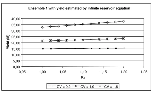
Ensemble 1 with yield estimated by infinite reservoir equation
The analysis shows (tables 4 to 6 and figures 3 and 4) that there is a positive trend in reservoir yield. Notice that this yield represents the maximum controllable yield in the basin. So, regarding to maximum regulation capacity, in case of hydrologically balanced changes (ensemble 1), the impact of global change in the reservoir will
Ensemble 1 estimated by Monte Carlo simulations
0,00 0,10 0,20 0,30 0,40 0,50 0,60 0,70
0,95 1,00 1,05 1,10 1,15 1,20 1,25
KX
Efficiency (
η)η)
CV = 0,2 CV = 1,0 CV = 1,6
Ensemble 1 estimated by Monte Carlo simulations
0,00 5,00 10,00 15,00 20,00 25,00 30,00 35,00
0,95 1,00 1,05 1,10 1,15 1,20 1,25
KX
Yield (M)
be slightly positive. Despite of that, the reservoir efficiency decreases in all cases studied.
Table 4. Values of annual yield (M) and reservoir efficiency (η) with 90% of reliability for an infinite reservoir in ensemble 1 (CV = 0.2)
KX µ (hm³/year) fE M (hm³/year) η =0.95 fM
1.00 42.58 0.36 32.74 0.73
1.02 43.43 0.36 33.26 0.73
1.04 44.28 0.37 33.78 0.73
1.06 45.13 0.37 34.29 0.72
1.08 45.99 0.38 34.80 0.72
1.10 46.84 0.38 35.31 0.72
1.12 47.69 0.39 35.81 0.72
1.14 48.54 0.39 36.31 0.71
1.16 49.39 0.40 36.81 0.71
1.18 50.24 0.40 37.30 0.71
1.20 51.10 0.41 37.79 0.70
Table 5. Values of annual yield (M) and reservoir efficiency (η) with 90% of reliability for an infinite reservoir in ensemble 1 (CV = 1.0)
KX µ (hm³/year) fE M (hm³/year) η =0.95 fM
1.00 42.58 0.36 21.40 0.48
1.02 43.43 0.36 21.62 0.47
1.04 44.28 0.37 21.83 0.47
1.06 45.13 0.37 22.04 0.47
1.08 45.99 0.38 22.25 0.46
1.10 46.84 0.38 22.45 0.46
1.12 47.69 0.39 22.64 0.45
1.14 48.54 0.39 22.83 0.45
1.16 49.39 0.40 23.02 0.44
1.18 50.24 0.40 23.20 0.44
1.20 51.10 0.41 23.38 0.44
Table 6. Values of annual yield (M) and reservoir efficiency (η) with 90% of reliability for an infinite reservoir in ensemble 1 (CV = 1.6)
KX µ (hm³/year) fE M (hm³/year) η =0.95 fM
1.00 42.58 0.36 14.90 0.33
1.02 43.43 0.36 14.98 0.33
1.04 44.28 0.37 15.06 0.32
1.06 45.13 0.37 15.13 0.32
1.08 45.99 0.38 15.20 0.31
1.10 46.84 0.38 15.26 0.31
1.12 47.69 0.39 15.32 0.31
1.14 48.54 0.39 15.38 0.30
1.16 49.39 0.40 15.43 0.30
1.18 50.24 0.40 15.49 0.29
Figure 3. Values of annual yield (M) with 90% of reliability for an infinite reservoir in ensemble 1 (CV = 0.2 to 1.6)
Figure 4. Values of reservoir efficiency (η) with 90% of reliability for an infinite reservoir in ensemble 1 (CV = 0.2 to1.6)
Ensemble 1 with yield estimated by infinite reservoir equation
0,00 0,10 0,20 0,30 0,40 0,50 0,60 0,70 0,80
0,95 1,00 1,05 1,10 1,15 1,20 1,25
KX
Efficiency (
η)η)
CV = 0,2 CV = 1,0 CV = 1,6
Ensemble 1 with yield estimated by infinite reservoir equation
0,00 5,00 10,00 15,00 20,00 25,00 30,00 35,00 40,00
0,95 1,00 1,05 1,10 1,15 1,20 1,25
KX
Yield (M)
Ensemble 2 with yield estimated by Monte Carlo simulations
Ensemble 2 embraces the scenarios where precipitation and evaporation increase in the same ratio (KX) and run-off increases in a rate KR, according to Aguiar’s rule
(Equation 6):
4 3
2 351,91 H -118,74 H
H 112,9 -H 28,53
R(mm)= × × + × × (6)
where H is the mean annual precipitation over the basin and R(mm) is the run-off in millimeters, for an unit basin. Using H=0.52 as initial condition, one can find the reference run-off for an unit basin (R°mm) equal to 25.02 mm. The other values of Rmm (for each precipitation H) are evaluated by Equation 6. The KR values are
obtained dividing the correspondent Rmm by R°mm. The mean annual inflow (µ) in each scenario KX is estimated by multiplying the mean annual inflow of the initial
conditions (42.58 hm³/year) by the correspondent KR. The results are showed in
table 7, 8 and 9 and figures 5 and 6..
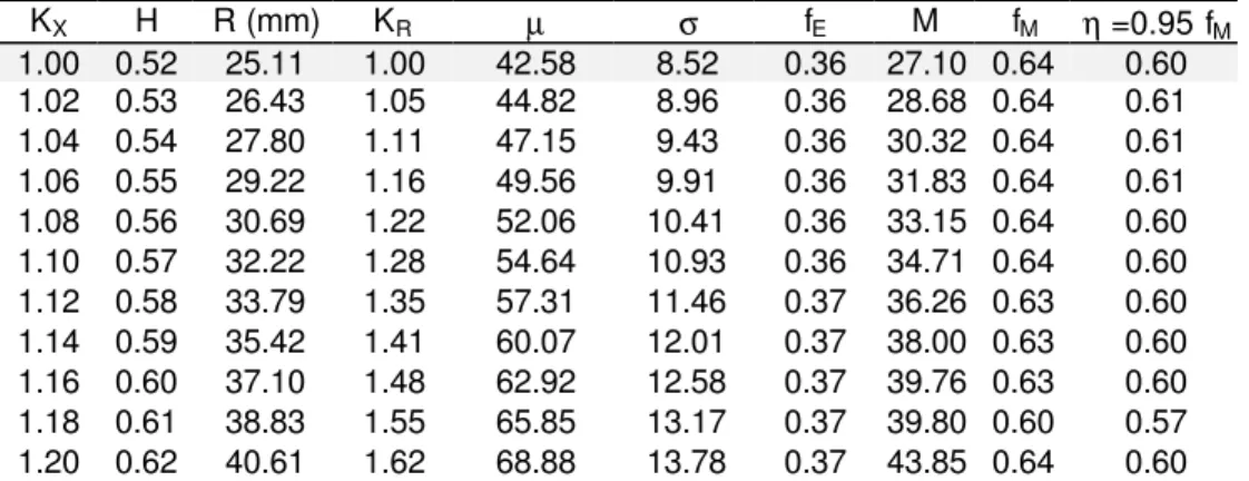
Table 7. Values of annual yield (M) and reservoir efficiency (η) for a 90% reliability, computed by Monte Carlo Simulations, in ensemble 2 (CV = 0.2)
KX H
(m) R (mm) KR µ σ fE M fM η =0.95 fM
1.00 0.52 25.11 1.00 42.58 8.52 0.36 27.10 0.64 0.60
1.02 0.53 26.43 1.05 44.82 8.96 0.36 28.68 0.64 0.61
1.04 0.54 27.80 1.11 47.15 9.43 0.36 30.32 0.64 0.61
1.06 0.55 29.22 1.16 49.56 9.91 0.36 31.83 0.64 0.61
1.08 0.56 30.69 1.22 52.06 10.41 0.36 33.15 0.64 0.60
1.10 0.57 32.22 1.28 54.64 10.93 0.36 34.71 0.64 0.60
1.12 0.58 33.79 1.35 57.31 11.46 0.37 36.26 0.63 0.60
1.14 0.59 35.42 1.41 60.07 12.01 0.37 38.00 0.63 0.60
1.16 0.60 37.10 1.48 62.92 12.58 0.37 39.76 0.63 0.60
1.18 0.61 38.83 1.55 65.85 13.17 0.37 39.80 0.60 0.57
1.20 0.62 40.61 1.62 68.88 13.78 0.37 43.85 0.64 0.60
Table 8. Values of annual yield (M) and reservoir efficiency (η) for a 90% reliability, computed by Monte Carlo Simulations, in ensemble 2 (CV = 1,0)
KX H (m) R (mm) KR µ σ fE M fM η =0.95 fM
1.00 0.52 25.11 1.00 42.58 42.58 0.36 11.15 0.26 0.25
1.02 0.53 26.43 1.05 44.82 44.82 0.36 11.68 0.26 0.25
1.04 0.54 27.80 1.11 47.15 47.15 0.36 12.34 0.26 0.25
1.06 0.55 29.22 1.16 49.56 49.56 0.36 13.12 0.26 0.25
1.08 0.56 30.69 1.22 52.06 52.06 0.36 13.66 0.26 0.25
1.10 0.57 32.22 1.28 54.64 54.64 0.36 14.28 0.26 0.25
1.12 0.58 33.79 1.35 57.31 57.31 0.37 14.73 0.26 0.24
1.14 0.59 35.42 1.41 60.07 60.07 0.37 15.42 0.26 0.24
1.16 0.60 37.10 1.48 62.92 62.92 0.37 16.19 0.26 0.24
1.18 0.61 38.83 1.55 65.85 65.85 0.37 16.90 0.26 0.24
Table 9. Values of annual yield (M) and reservoir efficiency (η) for a 90% reliability, computed by Monte Carlo Simulations, in ensemble 2 (CV = 1.6)
KX H (m) R (mm) KR µ σ fE M fM η =0.95 fM
1.00 0.52 25.11 1.00 42.58 68.13 0.36 4.63 0.11 0.10
1.02 0.53 26.43 1.05 44.82 71.72 0.36 4.96 0.11 0.11
1.04 0.54 27.80 1.11 47.15 75.44 0.36 5.22 0.11 0.11
1.06 0.55 29.22 1.16 49.56 79.30 0.36 4.44 0.09 0.09
1.08 0.56 30.69 1.22 52.06 83.29 0.36 5.70 0.11 0.10
1.10 0.57 32.22 1.28 54.64 87.42 0.36 6.04 0.11 0.10
1.12 0.58 33.79 1.35 57.31 91.70 0.37 6.03 0.11 0.10
1.14 0.59 35.42 1.41 60.07 96.11 0.37 6.32 0.11 0.10
1.16 0.60 37.10 1.48 62.92 100.67 0.37 6.65 0.11 0.10
1.18 0.61 38.83 1.55 65.85 105.36 0.37 7.02 0.11 0.10
1.20 0.62 40.61 1.62 68.88 110.21 0.37 7.29 0.11 0.10
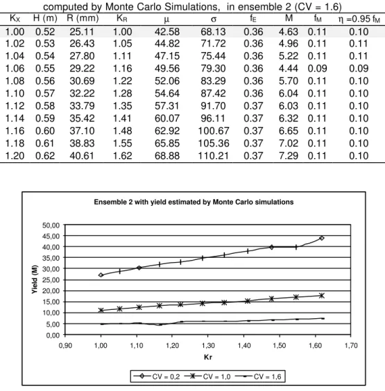
Figure 5. Values of reservoir yield (M) with 90% of reliability using Monte Carlo Simulation reservoir in ensemble 2 (CV = 0.2 to1.6)
As can be saw in tables 7, 8 and 9, there is a positive trend in water availability for KX - more accentuated for smaller CV’s. Considering CV=0.2, for instance, when
precipitation increases 4%, the reservoir yield increases 62%. That is, in the global change assumptions of ensemble 2, it is expected a reasonable gain in water availability. The reservoir efficiency, however, remain practically inalterable.
Ensemble 2 with yield estimated by Monte Carlo simulations
0,00 5,00 10,00 15,00 20,00 25,00 30,00 35,00 40,00 45,00 50,00
0,90 1,00 1,10 1,20 1,30 1,40 1,50 1,60 1,70
Kr
Yield (M)
Figure 6. Values of reservoir efficiency (η) with 90% of reliability using Monte Carlo Simulation reservoir in ensemble 2 (CV = 0.2 to1.6)
Ensemble 2 with yield estimated by infinite reservoir equation
The analysis showed that there is a positive trend in reservoir yield, independently of the CV assumed. Regarding to maximum capacity of regulation, in case of hydrologically balanced changes (ensemble 2), the impact of global change in the reservoir will be positive regarding to water availability. Regarding the efficiency, otherwise, it remains inalterable (tables 10, 11 and 12 and figures 7 and 8).
Table 10. Values of annual yield (M) and reservoir efficiency (η) for a 90% reliability for an infinite reservoir in ensemble 2 (CV = 0.2)
KX KR µ (hm³/year) fE M (hm³/year) η =0.95 fM
1.00 1.00 42.58 0.36 32.74 0.73
1.02 1.05 44.82 0.36 34.44 0.73
1.04 1.11 47.15 0.36 36.20 0.73
1.06 1.16 49.56 0.36 38.02 0.73
1.08 1.22 52.06 0.36 39.91 0.73
1.10 1.28 54.64 0.36 41.86 0.73
1.12 1.35 57.31 0.37 43.88 0.73
1.14 1.41 60.07 0.37 45.96 0.73
1.16 1.48 62.92 0.37 48.11 0.73
1.18 1.55 65.85 0.37 50.33 0.73
1.20 1.62 68.88 0.37 52.61 0.73
Ensemble 2 with yield estimated by Monte Carlo simulations
0,00 0,10 0,20 0,30 0,40 0,50 0,60 0,70
0,90 1,00 1,10 1,20 1,30 1,40 1,50 1,60 1,70
Kr
Efficiency (
η)η)
Table 11. Values of annual yield (M) and reservoir efficiency (η) for a 90% reliability for an infinite reservoir in ensemble 2 (CV = 1,0)
KX KR µ (hm³/year) fE M (hm³/year) η =0.95 fM
1.00 1.00 42.58 0.36 21.40 0.48
1.02 1.05 44.82 0.36 22.48 0.48
1.04 1.11 47.15 0.36 23.61 0.48
1.06 1.16 49.56 0.36 24.77 0.48
1.08 1.22 52.06 0.36 25.97 0.48
1.10 1.28 54.64 0.36 27.22 0.47
1.12 1.35 57.31 0.37 28.50 0.47
1.14 1.41 60.07 0.37 29.83 0.47
1.16 1.48 62.92 0.37 31.20 0.47
1.18 1.55 65.85 0.37 32.61 0.47
1.20 1.62 68.88 0.37 34.06 0.47
Table 12. Values of annual yield (M) and reservoir efficiency (η) for a 90% reliability for an infinite reservoir in ensemble 2 (CV = 1,6)
KX KR µ (hm³/year) fE M (hm³/year) η =0.95 fM
1.00 1.00 42.58 0.36 14.90 0.33
1.02 1.05 44.82 0.36 15.64 0.33
1.04 1.11 47.15 0.36 16.41 0.33
1.06 1.16 49.56 0.36 17.20 0.33
1.08 1.22 52.06 0.36 18.02 0.33
1.10 1.28 54.64 0.36 18.87 0.33
1.12 1.35 57.31 0.37 19.74 0.33
1.14 1.41 60.07 0.37 20.65 0.33
1.16 1.48 62.92 0.37 21.58 0.33
1.18 1.55 65.85 0.37 22.54 0.33
Figure 7. Values of reservoir yield (M) with 90% of reliability for an infinite reservoir in ensemble 2 (CV = 0.2 to1.6)
Figure 8. Values of reservoir efficiency (η) with 90% of reliability for an infinite reservoir in ensemble 2 (CV = 0.2 to1.6)
Ensemble 2 with yield estimated by infinite reservoir equation
0 , 0 0 1 0 , 0 0 2 0 , 0 0 3 0 , 0 0 4 0 , 0 0 5 0 , 0 0 6 0 , 0 0
0 , 9 0 1 , 0 0 1 , 1 0 1 , 2 0 1 , 3 0 1 , 4 0 1 , 5 0 1 , 6 0 1 , 7 0
Kr
Yield (M)
C V = 0 , 2 C V = 1 , 0 C V = 1 , 6
Ensemble 2 with yield estimated by infinite reservoir equation
0,00 0,10 0,20 0,30 0,40 0,50 0,60 0,70 0,80
0,90 1,00 1,10 1,20 1,30 1,40 1,50 1,60 1,70
Kr
Efficiency (
)
CONCLUSIONS
The results of this research regarding to impacts of global change in water availability in a typical reservoir in Northeast Brazil reach the following conclusions:
For the pessimistic scenario of hydrologically balanced changes called “ensemble 1” (precipitation, evaporation and inflows increasing at the same ratio) there are a positive trend in reservoir yield and a negative trend in reservoir efficiency in the present river basin topology. This behavior is also observed in the assumption of an infinite reservoir. The negative trend in reservoir efficiency is more accentuated for larger values of coefficient of variation of annual inflows.
For the optimistic scenario of hydrologically balanced changes called “ensemble 2” (precipitation and evaporation increasing at the same ratio, and inflows increasing according Aguiar’s polynomial rule) there is a positive trend in the reservoir yield for the present river basin topology as well as for the totally controlled basin. On the other hand, in both situations, no gains, or losses, are predicted in reservoir efficiency.
ACKNOWLEDGMENTS
The authors would like to thank CNPq and FUNCEME for supporting the research.
REFERENCES
AGUIAR, F.G.. Estudo Hidrométrico do Nordeste Brasileiro. Departamento Nacional de Obras Contra as Secas. Boletim Técnico. 36 n. 2 jul./dez 1978. Reimpressão .
CAMPOS, J.N.B. (1987). A Procedure for Reservoir Sizing on Intermittent Rivers Under High Evaporation Rate. Fort Collins, Colorado State University. PhD thesis.
CAMPOS, J.N.B., VIEIRA NETO, J. e QUEIROZ, E.A. (2000). Impacto Cumulativo da pequena açudagem: um estudo de caso do Açude Várzea do Boi, em Tauá, Ce. IN: V Simpósio de Recursos Hídricos do Nordeste, Natal, RN.
CAMPOS, J.N.B. (1996). Dimensionamento de Reservatórios: O Método do Diagrama Triangular de Regularização Edições UFC. Fortaleza 1996
CAMPOS, J. N. B.; IBIAPINA, N. G. (1997). Uma Equação para a Máxima Capacidade de Regularização em um Reservatório In. XII Simpósio Brasileiro de Recursos Hídricos , Vitória, ES. Associação Brasileira de Recursos Hídricos.
CAMPOS, J.N.B e STUDART, T.M.C. (2001). Variabilidades Climáticas e Tendências Hidrológicas em Climas Semi-Áridos. In: III Encuentro das Aguas, Santiago, Chile.