A closer look at the spatial exponential matrix specification

Contents lists available atScienceDirect

Spatial Statistics

journal homepage:www.elsevier.com/locate/spasta

A closer look at the spatial exponential

matrix specification

Erica Rodrigues

a,∗

, Renato Assunção

b

, Dipak K. Dey

c a_{Departamento de Estatística, Universidade Federal de Ouro Preto, Diogo de Vasconcelos,} 122, Ouro Preto, Brazil

b_{Departamento de Ciência da Computação, Universidade Federal de Minas Gerais,} Avenida Antônio Carlos, 6627, Belo Horizonte, Brazil

c_{215 Glenbrook Road, University of Connecticut, Storrs, CT 06269-4098, United States}

a r t i c l e i n f o

Article history:

Received 30 August 2013 Accepted 28 November 2013 Available online 4 December 2013

Keywords:

Exponential matrix Spatial autoregression Covariance matrix Spatial regression

a b s t r a c t

In this paper we analyze the partial and marginal covariance structures of the spatial model with the covariance structure based on a exponential matrix specification. We show that this model presents a puzzling behavior for many types of geographical neighborhood graphs, from the simplest to the most complex. In particular, we show that for this model it is usual to have opposite signs for the marginal and conditional correlations between two areas. We show these results through experimental examples and analytical demonstrations.

©_{2013 Elsevier B.V. All rights reserved.}

1. Introduction

Suppose we have a regionRpartitioned intondisjoint areasA1

,

A2

, . . . ,

Ansuch that

∪

ni=1Ai

=

R.

The data observed in each of these areas are, typically, counts, sums or some type of aggregated value of characteristics associated with the each of these units. In order to introduce the spatial dependence between them, we need to define a neighborhood structure according to the geographical arrangement of these areas. Once defined the neighborhood structure, we specify models reflecting the geographical location of the data. One recurrent approach relies on ideas from autoregressive time series models. A popular model that include this type of structure is the Simultaneous Autoregressive (SAR) model (Whitle, 1954). The SAR model is specified by a set of regression equations in which the dependent variable is the observation in a particular area and the explanatory variables are

∗_{Corresponding author. Tel.: +55 3188963607.}

E-mail address:ericaa_casti@yahoo.com.br(E. Rodrigues).

2211-6753/$ – see front matter©2013 Elsevier B.V. All rights reserved.

the observations on their neighbors. This system of equations is solved simultaneously inducing a multivariate normal distribution.

Letyibe a value observed in areaAi. The SAR model is determined by the simultaneous solution of

the set of equations given by:

Yi

=

µi

+

n



j=1

sij(Yj

−

µj)

+

ϵi

fori

=

1

, . . . ,

n

,

(1)

where

ϵi

are i.i.d. normally distributed with variance

σ

2

_{, µi}

₌

_E

₍

_{Yi), ands}

ijare parameter-dependent

constants withsii

=

0. IfY

=

(

Y1

,

Y2

, . . . ,

Yn), then the set of equations(1)leads to a multivariate normal distribution forY:

Y

∼

N



µ, σ

2

(

I

−

S

)

−1

(

I

−

ST

)



,

where

µ

=

(µ

1

, µ

2

, . . . , µn)

and the matrixSis composed by the constantssijconstrained in such a

way as to guarantee the existence of

(

I

−

S

)

−1.

The maximum likelihood estimator of the unknown parameters, including the parameter dependent matrix, is typically hard to obtain due to the constrained optimization and the need to deal with the determinant of the covariance matrix.LeSage and Kelley Pace(2007) present a new spatial model that bypass these numerical problems. This is a particular case of the proposal made byChiu et al.(1996) where general covariance matrices are expressed as the exponential function applied to a certain matrix. A major advantage of this definition is that it guarantees that the covariance matrix is always positive definite. Thus, it becomes unnecessary to put constraints on the parameter space during the estimation procedure to ensure that this property is satisfied. Another advantage is the simple way to obtain the precision matrix.

However, as we show in this paper, the exponential matrix covariance model has a major disadvantage when used in the spatial context. Mainly, this model is not flexible enough to incorporate many covariance patterns that one would expect to find in practice. The model is restricted to covariance patterns that have, in fact, non-intuitive aspects. The main point is that using this approach, in most practical situations, it will lead to opposite signs for the marginal and the partial correlations between pairs of neighboring areas. This limitation implies in an undesirable restrictive behavior for the stochastic structure of the data and therefore requires careful justification for its use. In Section2, we study the properties of this exponential covariance matrix in detail starting by describing the model proposed byLeSage and Kelley Pace(2007). Consider the partial correlation Cor

(

Yi,Yj

|

Y−ij),

given all the other variablesY−ijin the map. We prove in Section3that, for even-order neighboring

pairs, Cor

(

Yi,Yj

|

Y−ij)has the opposite sign as the marginal Cor

(

Yi,Yj), irrespective of the value of the

coefficients in the model. In Section4, we show that this behavior is non-intuitive and it is not allowed in the usual time series models. In irregular lattices, as those used in geographical data analysis, we showed in Section5that the non-intuitive sign change behavior of second-order neighbors is common although not guaranteed. In fact, we show that this happens for certain range of the exponential matrix parameters. Using matrix derivatives, we demonstrate that as the spatial correlation parameter increases, this puzzling behavior is intensified. More disconcerting, we show that, even for first-order neighboring areas in real maps, we can easily generate different signs for marginal and partial correlations. In Section7, we discuss the consequences of this behavior and present our conclusions.

2. Model definition

To guarantee that the normal distribution induced by the set of simultaneous equations(1)is proper, the matrix

(

I

−

S

)

must be of full rank. One possibility to ensure this property is to set S

=

ρ

Dand put restrictions on the space where the parameter

ρ

is defined. The matrixD can be specified in various ways. The two most common approaches are the following. In the first one, denoted byW, we define a binary matrix:Wijreceives value 1 if the areasiandjare neighbors, and

as a row standardized version ofW. That is,Dij

=

Wij/Wi+, whereWi+

=



jWij. The parameter

ρ

represents spatial association between areas. It can be shown that

(

I

−

ρ

D

)

is nonsingular if

ρ

∈



1

λ

1

,

1

λn



where

λ

1

<

0

< λn

are, respectively, the smallest and largest eigenvalues of the matrixD.

Considering the row standardizedDmatrix, we have that

λn

=

1. In this case the interval where

ρ

is defined is in the form

ρ

∈

(

1

/λ

1

,

1

)

. Under these conditions, it is possible to show that the matrix

(

I

−

ρ

D

)

−1_{can be expressed as}

(

I

−

ρ

D

)

−1

=

I

+

ρ

D

+

ρ

2D2

+

ρ

3D3

. . . .

(2)

The matricesDandDk_{can be seen as transition matrices, the first one in one step and the second ink}

steps.Dkalso represents thek-th order neighborhood. This means that we can go fromitojby passing throughkedges, and we cannot do this in less thanksteps. Therefore, from Eq.(2), we see that the influence of distant neighborhoods falls geometrically in this model.Assunção and Krainski(2009) analyzed how this decay influences the behavior of marginal correlations induced by the Conditional Autoregressive (CAR) model used as prior distribution in Bayesian models.Martellosio(2012) also addressed this problem focusing on SAR specification.

The idea of LeSage and Kelly Pace is to propose a model in which the influence of more distant neighborhoods falls more quickly. One possibility would be to replace

(

I

−

ρ

D

)

−1_{in the original version} of the model, by the convergent matrix series

I

+

α

D

+

α

2

2

!

D

2

₊

α

3 3

!

D

3

_{. . . .}

₍₃₎

Thek-th term in(2)is now divided byk

!

implying in a faster decrease towards zero and hence in a smaller impact of thek-th neighborhood in the infinite sum(3). This series is called exponential matrix and is denoted byeαD_{. It has interesting properties that are listed below. Consider two arraysXandY}

of dimensionsn

×

nand letaandbbe two scalars, then

e0

=

I

;

eaXebX

=

e(a+b)X

_;

ifXY

=

YXtheneY_eX

₌

_eX_eY

₌

_eX+Y

_;

ifYis invertible theneYXY−1

=

YeXY−1

.

In the model proposed byLeSage and Kelley Pace(2007) the covariance matrix is defined as

Σα

=

σ

2



e−αD′

e−αD



₍₄₎

therefore mimicking the SAR covariance matrix, whereDis an

×

nmatrix of spatial non-negative weights. As previously mentioned, typically it is considered thatDij

>

0 ifiandjare neighbors and Dij

=

0, otherwise.

The covariance model proposed byChiu et al.(1996) is more general and it is also based on an exponential matrix. They applied their model to analyze longitudinal data but the model could be applied in any regression context where one aims to model the covariance using the design matrix. Although we focus our paper on the spatial model suggested byLeSage and Kelley Pace(2007), the same problems we identified in this model are also present in the more general model ofChiu et al.

(1996). In particular, in longitudinal data, it is not reasonable that the marginal and partial correlations have opposite signs. This would mean, for example, that if the measurement of an individual at time

and partial autocorrelation functions will have both positive signs for any order of neighborhood taken into consideration.

We demonstrate in this paper that the definition proposed byLeSage and Kelley Pace(2007) can induce marginal and conditional correlations with opposite signs. This type of problem has been widely studied when dealing with dependence structure between variables and is known as Simpson’s Paradox (Pearl,2000;Wagner,1982). This paradox says that the sign of the correlation between two variables can be modified if we condition on a third variable. That is, the marginal correlation, without considering the third variable, has a different sign of the correlation obtained when conditioning in that variable.

This type of non-intuitive behavior for spatial models has been pointed out byBanerjee et al.(2003) (see p. 169) who say that for the SAR and conditional autoregression (CAR) models ‘‘transformation to (the covariance matrix)ΣY is very complicated and very non-linear. Positive conditional association

can become negative unconditional association’’. However, for SAR and CAR models such kind of behavior is observed only in cases of little practical interest, those in which there is a negative spatial association, or a repulsion, between the areas (Wall,2004;Assunção and Krainski, 2009;Martellosio,

2012). A simple explanation for this fact can be obtained from a result shown byJones and West(2005). This result guarantees that if all partial correlations have positive sign, then the marginal correlation will also be positive. In the specification of these models, for positive values of the spatial association parameter, the partial correlations between any pairs of areas are always positive. Thus, the marginal correlation will also have positive sign. Other puzzling results in the spatial case are explained away byAssunção and Krainski(2009) andMartellosio(2012). As we show in the next sections, for the model proposed byLeSage and Kelley Pace(2007), this change on signs occurs even when there is a positive association between the areas.

3. The case of regular lattices

The first case to be analyzed is a simple situation, a regular lattice. This means that the number of neighbors (ni) of each area is fixed and equal to 4, using the periodic boundary condition which

identifies opposite sides of the lattice wrapping it up as a torus. Let us assume that the matrixDis standardized, i.e.,

[

D

]

ij

=

1

/

niif areasiandjare neighbors and 0 otherwise. Let us also consider that

σ

2

=

1. AsD′

=

DandD′D

=

DD′we have that, in the exponential matrix model(4)

Σα

=

e−αD

′

e−αD

₌

_e−αD′−αD

₌

_e−2αD

_.

We know that, by definition of the exponential matrix,

e−2αD

=

I

−

(

2

α)

D

+

(

2

α)

2

2

!

D

2

₋

(

2

α)

3 3

!

D

3

₊

(

2

α)

4 4

!

D

4

₋

(

2

α)

5 5

!

D

5

_{+ · · ·}

_.

The termijof the matrixDk_{gives the probability that a random walk traveling in the adjacency}

graph leaves the areaiand reachesjinksteps. We know that, for a regular lattice, it is possible to go to an odd-order neighbor (first, third, fifth, etc.) only in an odd number of steps, and to a neighbor of even order (second, fourth, sixth, etc.) in an even number of steps. This means that, ifkis odd,

Dk_ij



>

0 ifiandjare neighbor of odd order

=

0 otherwise

and, ifkis even,

Dk_ij



>

0 ifiandjare neighbor of even order

=

0 otherwise.

So, ifiandjare neighbors of first order, theij-th element of the covariance matrix is given by

[

e−2αD

]

ij

= −

(

2

α)

[

D

]

ij

−

(

2

α)

3

3

!

[

D

3

_]

ij

−

(

2

α)

5

5

!

[

D

5

_]

ij

+ · · ·

(5)

We also know that the precision matrix (inverse of the covariance matrix) in this case is given by



e−2αD

−

1

₌

_e2αD

₌

_I

₊

₍

₂

_α)

_D

₊

(

2

α)

2

2

!

D

2

₊

(

2

α)

3

3

!

D

3

₊

(

2

α)

4

4

!

D

4

₊

(

2

α)

5

5

!

D

5

_{+ · · ·}

_.

As the sign of the conditional correlation is given by the opposite sign of the entries of the precision matrix, the sign of the conditional correlations between any pairs of areas is the opposite of the sign of

α

in regular lattices. For example, ifiandjare first order neighbors, theij-th element of the precision matrix

[

e−2αD

_]

−1

₌

_e2αD_{is given by}

[

e2αD

]

ij

=

(

2

α)

[

D

]

ij

+

(

2

α)

3

3

!

[

D

3

]

ij

+

(

2

α)

5

5

!

[

D

5

]

ij

+ · · ·

.

By comparing this expression with that presented in(5), we can see that the marginal and partial correlations betweeniandjhave the same sign.

Consider now a pair of second order neighbors,iandj. We have that theij-th element of the covariance matrix is given by

[

e−2αD

]

ij

=

(

2

α)

2

2

!

[

D

2

_]

ij

+

(

2

α)

4 4

!

[

D

4

_]

ij

+

(

2

α)

6 6

!

[

D

6

_]

ij

+ · · ·

,

(6)

which is equal to theij-th element of the precision matrix

[

e2αD

_]

ij

=

(

2

α)

2

2

!

[

D

2

]

ij

+

(

2

α)

4

4

!

[

D

4

]

ij

+

(

2

α)

6

6

!

[

D

6

]

ij

+ · · ·

.

Comparing this expression with(6)we notice that the marginal correlation betweeniandjis always positive, but the partial correlation is always negative since it is the opposite sign of the precision matrix. This same behavior can be observed for all neighbors of even order. That is, for any pair of neighbors of this type, the marginal correlation between them will always be positive, but when we condition on other areas of the map this correlation turns out to be negative.

This is not a reasonable result for a model of spatial dependence. Whereas a marginal positive correlation means that if areaihas a value above its average, then areajwill also tend to have a value higher than expected. If we consider the values of all the other areas in the map to be known, the fact that the areaihave a value above its average, leads areajto have a value below its average. This happens only with even-order neighboring pairs and does not depend on the value of the conditioning variables.

For neighbors of even order we observe yet another strong constraint of this model. It only allows the existence of marginal positive correlations between neighbors of this type. That is, neighbors of second, fourth, sixth order can only be positively correlated regardless of the value of

α

.

Let us now see what are the consequences of these results for the conditional expectations, since the conditional expectation has a slightly more direct interpretation than the conditional correlation. Consider a Gaussian Markov Random Field whose precision matrix is denoted byQwith entriesQij

and whose mean vector

µ

is zero. It is known that the conditional expectation of the random variable

at a sitei, given the rest of the map (Y−i) can be obtained from the following expression

E

(

Yi

|

y−i)

= −

1

Qii



j

Qijyj. (7)

We have seen that, for the case of the regular lattice, ifiandjare neighbors of odd order,Qij

<

0

and ifiandjare neighbors of even order,Qij

>

0. From Eq.(7), if we want to predict the value of

the variableYusing the observed values of its neighbors, those from neighbors of odd order will give a positive contribution, while those from neighbors of even order enter with a negative weight in the expectation. That does not seem reasonable, since the marginal correlations ofiwith each of its neighbors have positive sign, so they should all have a positive weight in the conditional mean.

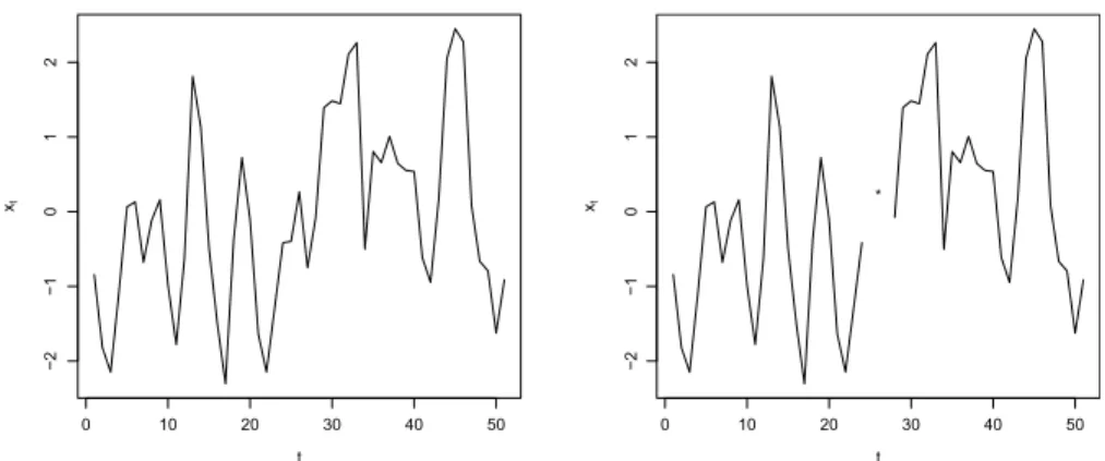
Fig. 1. Time series with 51 observations simulated (left) and simulated series removing observations of orders 25 and 27 (right).

In order to better understand the meaning of this sign change between marginal and conditional correlations, we present in the following section a short simulation study for the one-dimensional case.

4. The case of unidimensional lattices

The goal of this section is to show visually the kind of data that are generated when considering the covariance structure proposed byLeSage and Kelley Pace(2007). To facilitate the understanding and the graphic presentation, let us consider the case in which data is observed over time. We set the parameters

σ

2

₌

_{1 and}

_α

_{= −}

_{1 and generate a time series with 51 observations. The neighborhood} structure is a Markov chain of order one. The series generated is shown on the left ofFig. 1. Two observations were deleted and their values were resampled from the conditional distributions of these two variable points in time, given the rest of the series. The graph on the right panel ofFig. 1

shows the series with the two missing observations. In other words, we have a set of observations

x1

,

x2

, . . . ,

x51. We throw away the values ofx25andx27and consider these positions as if they were missing observations from our database. We know that the conditional distribution of the vector

(

X25

,

X27

)

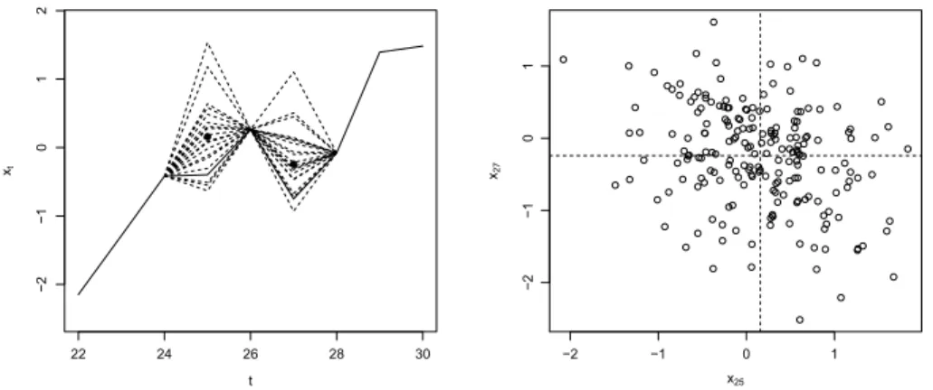
, given the rest of the series, is a bivariate normal. We generate some pairs of observations with such distribution to visually check their relationship. InFig. 2, the graph on the left panel shows in solid line the original series and the dashed line shows the values resampled from the conditional distribution. The points marked in black represent the values of the conditional expectation. It is observed that, as expected, if the values of one of the two selected points is below the conditional expectation, the other tends to be above its conditional expectation and vice versa.Fig. 2also shows the scatter plot generated from various observations for these two variables. We note that there is a negative correlation between the two variables, which was already expected since the two sites are neighbors of second order. In addition, for many points generated, if the observation of one site is below (above) its conditional mean, the observation of the other is above (below).

In order to visually contrast the behavior of the series generated from the analyzed model with the behavior of a classical ARIMA model, we generate 51 observations of an autoregressive process of order 2. The model parameters were set at 0.3 and 0.4 and the variance was fixed at

σ

2

₌

_{1. The data} were generated in the same way as was done in the previous case. The graphs on the left panel ofFig. 3

show the original series in solid line and observations generated through conditional distributions in dashed line. The black dots mark the conditional expectation. The right hand side ofFig. 3shows the scatter plot of observations generated from the conditional distribution. Unlike what happens in the previous case, there is clearly a positive association between the observations in the two sites.

5. Spatial irregular lattice

Fig. 2. Series generated, the dashed lines represent 20 observations generated from the conditional distributions and dots mark the conditional expectation (left). Scatter plot of five observations generated from the conditional distribution (right).

Fig. 3. Time series generated from an autoregressive process of order 2. Dashed lines represent the 20 observations generated from the conditional distributions and the points mark the conditional expectations (left). Scatter plot of 200 observations generated from the conditional distribution (right).

additional counterintuitive results. In this case we observe that the change of signs occurs even between first order neighbors. This situation is illustrated by the map of Iowa.

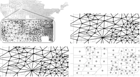
The map analyzed is shown inFig. 4. The neighborhood criterion used was the adjacency between areas, i.e., two areas are considered neighbors if, and only if, they share boundaries. The neighborhood matrix is specified as a binary matrix, which takes only values zero and one. We fix

α

= −

1

, σ

2

₌

₁ and hence the covariance matrix is of the form

Σα

=

eW

′

eW

,

whereWis a binary matrix such that

[

W

]

ij

=

1 ifiandjare neighbors, and zero otherwise.

Fig. 4. Iowa map representing marginal and conditional correlations between pairs of neighboring areas. The first figure shows the map of Iowa with links representing neighbors of the first order. The second shows connections between neighbors of first order that have marginal positive correlation. The third figure shows connections between pairs of neighboring areas that have positive conditional correlation. The fourth figure shows connections between pairs of areas that have negative conditional correlations.

Real maps often have areas of very different sizes, inducing very irregular graphs. This situation is more difficult to be analyzed because the topology of the graph becomes more complex.

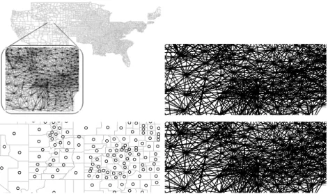
To illustrate this kind of situation, let us consider the map used in the application presented by

Fig. 5. First-order neighbors with positive marginal correlation, with positive partial correlation and with negative partial correlation.

in order to facilitate visualization. The value estimated for

α

in the application was

−

0.74 and this is the value used here. We adopted one of theDmatrices used by those authors, the row-standardized matrix.

The second graph inFig. 5 shows some of the pairs of neighbors that have marginal positive correlation. All first-order neighbors have this property. This was expected because for

α <

0 all the terms of the covariance matrix are positive. The first graph of the second line in the same figure shows the connections between first-order neighbors that have positive partial correlation. These are all neighbors of first order, i.e., in this case there is no change of sign. The last graph of this figure shows connections between first-order neighbors that have negative partial correlation, i.e., no pair of neighbors, which confirms the observation made previously. Differently fromFig. 4, we have no links between adjacent areas here. The reason is thatFig. 4adopts the binary adjacency matrix forD while here we use the row standardized matrix.

The first graph inFig. 6shows links between neighbors of second order. The second graph of this figure shows the pairs of second-order neighbors that have positive marginal correlation. As in the first-order neighborhood case, the correlation between any pair of areas is positive. The first graph in the second row ofFig. 6shows the connections between pairs of neighbors of second order that have positive partial correlation, i.e., no pair of neighbors. The bottom right graph shows the connections between second-order neighbors that have negative partial correlation. For this kind of neighbors, there is change of signs for all pairs. This behavior is repeated in general to neighbors of even order.

The correlations for this map behave in the same way that in the regular graph. Analyzing other maps, with completely different topological structure, with this same value for

α

, the same behavior was observed. We will see that this occurs because, as the value of

α

is small, the first order neighborhood pairs dominate the covariance and precision matrices.

To understand why this behavior occurs for any kind of map, we remind that the covariance matrix of the model is given by

σ

2e−αD′e−αD

.

Ignoring the variance term

σ

2_{and using the definition ofe}−αD_{, this product can be written as}



I

−

α

D′

+

α

2

2

!

D ′2

₋

α

3

3

!

D ′3

_{+ · · ·}

 

I

−

α

D

+

α

2

2

!

D

2

₋

α

3 3

!

D

3

_{+ · · ·}



.

Fig. 6. Second-order neighbors with positive marginal correlation, with positive partial correlation and with negative partial correlation.

is given by

(σ

2

)

−1eαD_eαD′

_.

Again using the definition ofeαD_{we get}



I

+

α

D

+

α

2

2

!

D

2

+

α

3

3

!

D

3

+ · · ·

 

I

+

α

D′

+

α

2

2

!

D ′2

+

α

3

3

!

D ′3

+ · · ·



.

If

α

is negative, we have the product of two summations involving positive and negative terms. Thus, the terms of the precision matrix can be positive or negative, depending on which array dominate the sum. We can rewrite the product as

I

+

α

D′

+

α

D

+

α

2

2

!

D ′2

₊

α

2

2

!

D

2

₊

_α

2_D′_D

_{+ · · ·}

_.

₍₈₎

Since

α

is small andDis limited between

[

0

,

1

]

, askincreases the terms

α

k

k

!

D

k _and

α

k

k

!

D ′k

go to zero. Therefore, the sum presented in(8)will be dominated only by the smaller exponents. Consider the case where two areasiandjare first-order neighbors. The terms

[

D

]

ijand

[

D′

]

ijare both

greater than zero and the sum in(8)is dominated by the terms

α

D′

+

α

D

.

As we are considering

α <

0, this sum is smaller than zero, which implies a positive correlation conditional. That is, ifiandjare first-order neighbors, marginal and conditional correlations have the same sign as we had already observed in the example.

Consider the case in whichiandjare second-order neighbors. In this case, we have

[

D

]

ij

= [

D′

]

ij

=

0, but

[

D2

]

ijand

[

D′2

]

ijare both greater than zero. Therefore, the sum in Eq.(8)is dominated by the

terms

α

2 2

!

D

′2

₊

α

2 2

!

D

2

₊

_α

2_D′_D

_.

Fig. 7. Correlation between first order neighbors for different values ofα.

conditional correlations have opposite signs. Hence, the behavior observed in the previous example is not restricted to the neighborhood structure defined before. For a small value of

α

, whatever map is considered, there will be change of signs in the correlations of second order neighbors.

6. How the partial correlation varies with

α

The way the partial correlation varies with

α

also shows some non-intuitive aspects. According to

LeSage and Kelley Pace(2007) the relationship between the parameter

α

of the proposed model and the parameter

ρ

of the SAR model is given by

α

≈

ln

(

1

−

ρ).

As the values of

ρ

with practical interest are

ρ >

0, we observe two important points from this relationship. The first one is that the values of

α

that have practical interest are

α <

0. The second one is that

α

decreases as

ρ

increases. Taking this into consideration, it would be reasonable that the marginal and conditional correlations have a decreasing behavior with respect to the parameter

α

. We will see here that, for the case of conditional correlations, this is not true.

Considering again the same map used byLeSage and Kelley Pace(2007), we find the values of the conditional correlations for different values of the parameter

α

. We will check first how is this relationship for pairs of sites that are neighbors of first order.Fig. 7presents the values of the correlations between first-order neighbors for

α

ranging from

−

1 to 0. Therefore, the conditional correlation decreases with the values of

α

. As explained earlier, this is a reasonable behavior, because it means that, as the spatial association between areas becomes stronger, the conditional correlation between certain pairs of areas will grow. For example,

α

=

0 is equivalent to

ρ

=

0, and this means independence between the areas. In this case, from the graph, we see that the partial correlation between the neighbors of first order is zero. For

α

= −

1 we have

ρ

≈

0

.

632, i.e., there should be an increase in the partial correlation between the areas. The graph presented inFig. 7shows that this is what happens.

Fig. 8. Correlation between neighbors of second order for different values ofα.

We can explain why this non-intuitive behavior happens for second order neighbors. Recall that the precision matrix is given by

σ

2eαD_eαD′

_.

Take derivatives of this product of matrices with respect to the parameter

α

:

deαD_eαD′

d

α

=

deαD

d

α

e

αD′

₊

_eαDdeαD′

d

α

.

Using

deαD

d

α

=

De

αD

we have

deαD_eαD′

α

=

De

αD_eαD′

₊

_eαD_D′_eαD′

_.

Using the definition ofeαD_{, this derivative becomes}

D



I

+

α

D

+

α

2D 2

2

!

+ · · ·

 

I

+

α

D′

+

α

2D ′2

2

!

+ · · ·



+



I

+

α

D

+

α

2D 2

2

!

+ · · ·



D′



I

+

α

D′

+

α

2D ′2

2

!

+ · · ·



which can be rewritten as

D

+

α

DD′

+

α

D2

+

α

2D2D′

+

α

2D 2

2

!

+ · · · +

D

′

₊

_α

_DD′

₊

_α

_D′2

₊

_α

2_DD′2

₊

_α

2D′2 2

!

+ · · ·

.

As this sum converges absolutely, we can change the order of summation. Assuming that

α

is small, we can ignore the terms with power greater than or equal to three and obtain

(

D

+

D′

)

+

α(

DD′

+

D′D

+

D2

+

D′2

)

+

α

2



D2D′

+

DD′2

+

D

2

2

!

+

D′2 2

!

+ · · ·



.

derivative is positive. That is, the conditional correlation increases when the parameter

α

decreases. Remember that the conditional correlation sign has the opposite sign of each term of the precision matrix. Therefore, as the spatial association between the areas increases (

α

→ −∞

), the conditional correlation between all neighbors of first order increases. On the other hand, ifiandjare second order neighbors, the first term of the sum is zero and the second term is nonzero and dominates the sum. Since, in general, we are interested in the case where

α <

0 this sum assumes a negative value. This means that if two areas are second-order neighbors, the conditional correlation between them decreases as the parameter

α

decreases. That is, as the spatial association between the areas increases, the conditional correlation between the second order neighbors gets stronger. However it gets stronger negatively, which is counterintuitive, since the increase in spatial association is leading to conditional repulsion between the areas.

7. Conclusion

We show in this paper that the spatial model where the covariance structure depends on an exponential matrix has some important non-intuitive aspects. Despite the advantages pointed out by

LeSage and Kelley Pace(2007), especially with regard to computational efficiency, the puzzling results shown here should be taken into account when considering this model. The type of non-intuitive behavior that we found in the exponential matrix model can also be observed for other widely used models, such as CAR and SAR models. However, in the case of the latter models, it only occurs when the spatial dependence parameter has a negative sign, i.e., a case with little applicability to real problems. As for the model proposed inLeSage and Kelley Pace(2007), this behavior is usually observed in situations of practical interest. Therefore, the application of this model should be done with caution, since the results may reflect a type of spatial dependence that has difficult practical interpretation.

Acknowledgment

The authors would like to thank CNPq, Capes and FAPEMIG for financial support.

References

Assunção, R., Krainski, E.,2009. Neighborhood dependence in Bayesian spatial models. Biom. J. 51 (5), 851–869.

Banerjee, S., Gelfand, A.E., Carlin, B.P.,2003. Hierarchical Modeling and Analysis for Spatial Data. CRC Press.

Chiu, Y.M.T., Leonard, T., Tsui, K.,1996. The matrix-logarithmic covariance model. J. Amer. Statist. Assoc. 91 (433), 198–210.

Jones, B., West, M.,2005. Covariance decomposition in undirected Gaussian graphical models. Biometrika 92 (4), 779–786.

LeSage, J.P., Kelley Pace, R.,2007. A matrix exponential spatial specification. J. Econometrics 140 (1), 190–214.

Martellosio, F.,2012. The correlation structure of spatial autoregressions. Econometric Theory 28 (6), 1373.

Pearl, J.,2000. Causality: Models, Reasoning and Inference, Vol. 29. Cambridge Univ. Press.

Wagner, C.H.,1982. Simpson’s paradox in real life. Amer. Statist. 36 (1), 46–48.

Wall, M.,2004. A close look at the spatial structure implied by the car and sar models. J. Statist. Plann. Inference 121, 311–324.