A SYSTEMATIC APPROACH TO CONSTRUCT CREDIT RISK FORECAST MODELS
Lisiane Priscila Rold˜ao Selau
1*and Jos´e Luis Duarte Ribeiro
2Received March 2009 / Accepted July 2010
ABSTRACT.Due to the recent growth in the consumer credit market and the consequent increase in default indices, companies are seeking to improve their credit analysis by incorporating objective proce-dures. Multivariate techniques have been used as an alternative to construct quantitative models for credit forecast. These techniques are based on consumer profile data and allow the identification of standards concerning default behavior. This paper presents a methodology for forecasting credit risk by using th-ree multivariate techniques: discriminant analysis, logistic regression and neural networks. The propo-sed method (deemed the CRF Model) consists of six steps and is illustrated by means of a real applica-tion. An important contribution of this paper is the organization of the methodological procedures and the discussion of the decisions that should be made during the application of the model. The feasibility of the approach proposed was tested in a program for granting credit offered by a network of pharmacies. The use of the models for forecasting credit risk greatly reduces the subjectivity of the analysis, by establishing a standardized procedure that speeds up and qualifies credit analysis.
Keywords: credit analysis, forecast model, credit risk.
1 INTRODUCTION
The credit market for low-income individuals in Brazil displays paradoxical characteristics. On the one hand, large numbers of individuals receive an income which makes it difficult for them to balance their basic domestic budget. On the other, many companies offer the promise of easy credit at a minimum bureaucracy (Silva, 2006).
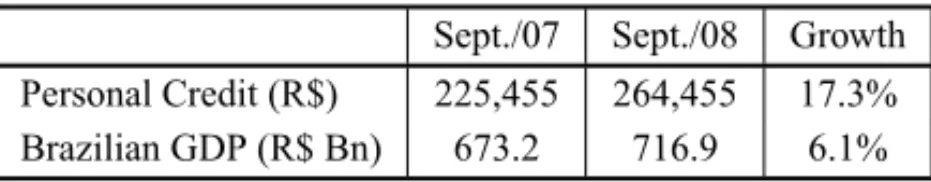
According to Pereira (2006), the growth of credit in recent years has been alerting credit analysts to a period of turbulence that may well be in the offing. Table 1 presents information on the growth of credit and GDP in Brazil. A disparity is observed among the numbers, due to the increase in the use of personal credit being much larger than the increase in GDP.
*Corresponding author
1Department of Mathematics and Statistics (DME), Universidade Federal de Pelotas (UFPel), Pelotas, RS, Brazil. E-mail: [email protected] / [email protected]
Table 1– Comparison of credit indicators and GDP in Brazil.
Sept./07 Sept./08 Growth Personal Credit (R$) 225,455 264,455 17.3% Brazilian GDP (R$ Bn) 673.2 716.9 6.1%
Source: ACREFI and INESC.
The growth in demand for personal credit in Brazil has been revolutionizing this market, thus companies in this sector are adapting themselves to remain at the forefront of the opportuni-ties. The phenomenon has caused a re-engineering in credit systems with regard to the role of technology in granting credit (Pereira, 2006).
Companies that grant credit are investing in better credit analysis, so as to avoid working with clients who pose a risk, thus reducing the default rate. Therefore besides the experience of the analyst, they are using methods and techniques that assist in the task of deciding whether a client is creditworthy. Recently, risk management has come to occupy a prominent position in financial administration, particularly as a result of the expansion of credit, of market growth and of globalization (Bueno, 2003).
According to Steineret al. (2007), making the correct decision as to granting credit is essential
for the survival of financial institutions. Any error in the decision to grant credit may mean that a single operation promotes a loss equivalent of the gain obtained in dozens of other successful transactions, since non-receipt represents the total loss of the amount lent. Therefore, it is impor-tant to forecast and reduce default, since the losses on unsuccessful credit will have to be covered by charging high interest rates on new lines of credit.
As Schrickel (1997) states, risk analysis involves the ability to make a credit decision in a sce-nario of uncertainties, constant changes and incomplete information. This ability depends on the capacity to logically analyse often complex situations, and reach a conclusion that is practical and feasible to implement.
In many companies, assessing creditworthiness is based on a variety of information from various sources. Managers analyse this information in a subjective way and often cannot explain the decision making processes, although they do manage to pinpoint the factors that influence deci-sions. Moreover, these environments are dynamic, with constant changes, and decisions must be
made quickly (Mendes Filhoet al., 1996).
propose a systematic approach to build credit risk forecast models so as to grant personal credit. The approach, deemed CRF Model, uses different analysis methodologies, in particu-lar, discriminant analysis, logistic regression and neural networks, and it is illustrated by means of a practical application.
This article is organized into four sections. After this introduction, the Section 2 provides the theoretical foundation, in which a brief outline on forecast credit risk model is given. Section 3 details the systematic approach proposed for building CRF models. Section 4 describes the background and the results of an applied study in which the systematic approach was used. The last section of the paper presents final considerations, including the main conclusions drawn.
2 MODELS FOR FORECASTING CREDIT RISK
Knowing the likelihood of a client honoring his/her commitments is essential information when taking a decision in regard to granting credit. Financial institutions could have an increase in their profits if the criteria used for granting credit were more objective. Possessing a classification provided by a model that forecasts credit risk, the company can have a preliminary diagnosis of the probable behavior of a new client, approving or not the demanded credit (Vasconcellos, 2004).
Steiner et al. (2007) stress that quantitative forecasting models are widely used to aid credit
analysis, and have the advantages of: (i) increasing the number of clients worthy of having the credit approved, thus increasing profits; (ii) increasing the number of those not worthy of re-ceiving the credit, thus reducing losses; (iii) analyzing credit applications faster; (iv) subjective criteria being replaced with objective decisions; and, finally, (v) requiring fewer people to ma-nage credit transactions.
Caouetteet al.(1999) argue that scoring systems for credit risk are important for placing, at the
disposal of the creditor, knowledge that would not otherwise be readily available. These authors add that there is a great competitive advantage in using models, because an integrated scoring system allows operations to take place in different geographical regions, involving several people, and even then, maintaining objectivity in decisions.
Models for risk forecast are tools that support credit on a very large scale, which is characterized by evaluating a large number of requests for small amounts, since market competition requires quick decisions. The analyst inputs the data from his potential client into the credit system, and immediately, the computer provides information as to credit approval. Indeed, the statistical methods used to construct the model take into consideration the institution’s record with its clients, thus enabling the identification of the characteristics that differentiate the good from the bad payer (Silva, 2006).
Some authors such as Singh (2003) and Caouetteet al.(1999) cited multivariate statistical analy-sis as a powerful tool in assessing the risk of non payment present when granting credit. One of the advantages of using statistical techniques to develop scoring systems is that the weights to be assigned to risk variables are determined by statistical calculations and processes, which excludes the subjectivity inherent at the moment of analysis or even the state of mind of the credit analyst.
After assigning numerical values to each selected applicant characteristic or risk variable, a score is obtained that will determine in a standardized, consistent and objective way, based on the calculated probability of repayment, if the credit may be granted or should be refused (Santos, 2000).
There are several techniques for building credit risk forecast models. Among the possible methods are: multiple linear regression, linear programming, genetic algorithms, decision tree, discriminant analysis, logistic regression, neural networks and, more recently, survival analysis
as set out in the study of Andreevaet al.(2007).
The combined use of techniques is also promising. Scarpel & Milioni (2002) combined a logit type econometric model with an integer linear programming model, with the aim of assisting credit analysis by using the estimated probability of companies solvency, thus minimizing the sum of opportunity and non payment costs. The authors concluded that the combined use of these models made it possible to eliminate the limitations found when they are used in isolation in decisions to grant credit.
3 SYSTEMATIC FOR DEVELOPING THE CRF MODEL
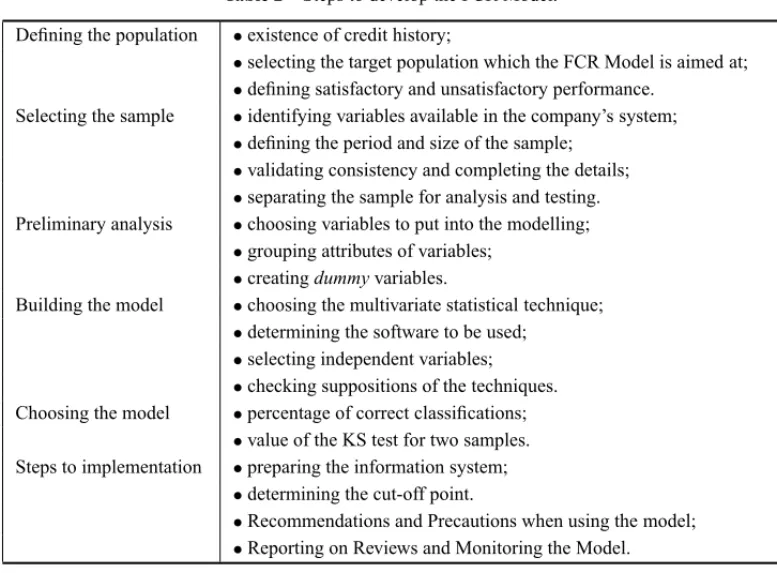
The systematic approach proposed for developing credit risk forecast models consists of six steps (see Table 2). The steps for building the CRF Model are explained one by one, and range from the first details needed to start the study to the steps for implementing the model.
3.1 Defining the population
The first step of the approach proposed includes defining the population and comprises the following steps: (i) availability of a credit history; (ii) selecting the target population at which the CRF model is aimed; (iii) defining satisfactory and unsatisfactory performance.
The basic assumption for building credit risk forecasts models is that clients sustain the same pattern of behavior over time (Gouvˆea & Gonc¸alves, 2006). Therefore, given that model building is exclusively based on company’s experience with using credit, all the data used in development come from business records. Sample data must comprise all information known about the clients at the time of granting credit, and also, their subsequent status as good and bad payers.
Table 2– Steps to develop the FCR Model.
Defining the population •existence of credit history;
•selecting the target population which the FCR Model is aimed at;
•defining satisfactory and unsatisfactory performance.
Selecting the sample •identifying variables available in the company’s system;
•defining the period and size of the sample;
•validating consistency and completing the details;
•separating the sample for analysis and testing.
Preliminary analysis •choosing variables to put into the modelling;
•grouping attributes of variables;
•creatingdummyvariables.
Building the model •choosing the multivariate statistical technique;
•determining the software to be used;
•selecting independent variables;
•checking suppositions of the techniques.
Choosing the model •percentage of correct classifications; •value of the KS test for two samples.
Steps to implementation •preparing the information system;
•determining the cut-off point.
•Recommendations and Precautions when using the model;
•Reporting on Reviews and Monitoring the Model.
So as to construct the model, what must be defined initially are the concepts of acceptable and unacceptable credit performance. According to Gouvea and Gill (2006), besides good and bad clients, there are also clients who should be excluded from the analysis, such as, for example, clients who work in the company and indeterminate clients, who are on the borderline between those who would be considered good or bad, without a position being defined regarding pay-ments. In practice, when constructing the model, companies normally consider only good and bad clients, due to the ease of working with models which give a dichotomous response.
Thus, there are four groups that should be separated in the total of credits granted: (i) clients who have never used the credit – non-users; (ii) clients who pay with little or no delay – good payers; (iii) clients banded as making intermediate delays in payments – indeterminate payers; and (iv) clients who accumulate considerable delay – bad payers. The definition of considerable delays should be set by the grantor, who will define the delays that can be accepted by the business. In building the model, only the groups of good and bad clients are used in order to accentuate profile separation and to reinforce the analysis.
3.2 Selecting the sample
The analysis of the information contained in companys database can be made by detailed ob-servation of credit proposals. Among the possible pieces of information selected, also called demographic variables, are: gender, age, level of education, marital status, type of occupation, type of residence, length of current employment, and so forth (Mester, 1997). Lewis (1992) sug-gests that the inclusion in the credit proposal of items of information considered important for future assessment of model adequacy should be carefully evaluated.
To define the period from which the sample should be extracted, it is necessary to observe a time between granting the credit and checking clients payment performance. Lawrence (1992) suggests that the clients who will be part of the sample have been included for at least 12-18 months. This elapsed time is usually sufficient to: (i) check the occurrence of delays and non payments, which define the bad client; and (ii) consolidate the payment behavior of the good client.
When using multivariate techniques, the sample size depends on the number of independent va-riables that will be part of the study for building the final model, and, especially, if the sample
adequately covers most of the combinations that can be generated from these variables. Hairet
al.(2005) suggest using a ratio of 20 observations for each independent variable included in the
model. The sample size in most cases is not a problem, because when it comes to businesses that grant personal credit, there usually is an abundance of historical data.
When there is a database, an exploratory analysis is conducted, in which the contents of all fields are analyzed. At this point, completion, consistency of the fields and presence of missing observations should be checked. Inconsistent or atypical data should be eliminated.
One final point to be considered concerning sample is the issue of the division between the analysis sample and the testing sample in order to avoid possible bias. According to Assaf Neto & Brito (2005), when testing the model with the same sample used in its construction, it might be concluded that its performance is good when, in fact, it may work well only for these specific set of observations. Therefore, tests are needed to check if the forecasting power of the model is maintained for other samples coming from the same population.
There are no fixed rules to dividing the sample. Hairet al.(2005) argue that the choice regarding
the division of the sample should be left to the researcher. Due to the greater importance that model building has over model testing, it is proposed to divide the total sample as suggested by Haykin (2001): 80% of the total sample for analysis and 20% for testing the final model. The separation of the samples is done via a computational routine, generating a uniformly distributed random variable to allocate, at random, cases to the respective samples.
3.3 Preliminary analysis
The preliminary analysis includes the following steps: (i) choosing variables to put into the modelling; (ii) grouping attributes of variables; (iii) creating dummy variables.
By using contingency tables, a calculation is made of the relative risk (RR) associated to the levels of the independent variables, by dividing the percentage of good clients by the percentage of bad ones for each level. The more the percentages of good and bad clients differ for the levels of a single variable, the greater the usefulness of this variable for the prognosis of future perfor-mance (Lewis, 1992). For example, if the same fraction of good and bad clients are homeowners or rent their home, this variable provides no information that may help to establish the probability of a client turning out to be a good or bad payer.
For variables with many possible levels, such as, for example, Zip code and Profession, clusters are necessary. This is done with the aim of decreasing the number of levels to be analyzed and, especially, to obtain representativeness in the clusters in order to increase the chance of their being part of the final model. The measurement used to form these clusters is also the result of the relative risk.
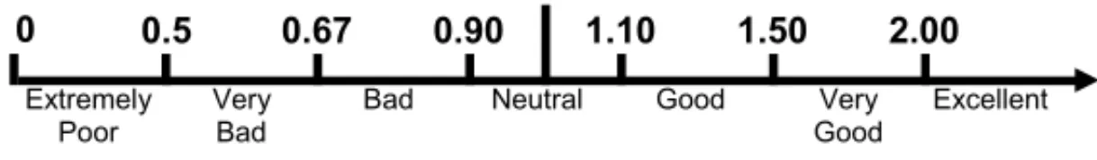
As a general rule, the attributes are divided according to the value of the relative risk into the
following classes: extremely poor (RR < 0.50); very bad (RR between 0.50 and 0.67); bad
(RR between 0.67 and 0.90); neutral (RR between 0.90 and 1.10); good (RR between 1.10 and 1.50); very good (RR between 1.50 and 2.00); and excellent (RR greater than 2.00), as shown in Figure 1. Levels classified as neutral are not used in the analysis, since they are not greatly different from the good and bad groups (Lewis, 1992).
Very Good
Excellent Very
Bad
Bad Neutral
Extremely Poor
1.10 1.50 2.00
0.90
0 0.5 0.67
Good
Figure 1– Classes of relative risk to be grouped.
After selecting the levels that will be part of the multivariate analysis, a dummy variable is created
for each one (e.g., each level of education will be a dummy variable). This variable assumes only
two values (0 or 1). By using this artifice, problems are avoided arising from the nonlinearity of the attributes in the calculation of the multivariate analysis.
3.4 Construction of the model
The construction of the model comprises the following steps: (i) choosing the multivariate statis-tical technique; (ii) determining the software to be used; (iii) selecting the independent variables; and (iv) checking assumptions of the techniques.
Once the data have been reduced to cluster levels, carefully chosen for all features, and the respective dummies created, each analyst chooses the method to be used for modelling. This study proposes the use of discriminant analysis, logistic regression and neural networks. Such methods were chosen because they are among the most widely used for building credit models (Desaiet al., 1996; Almeida & Dumontier, 1996; Armingeret al., 1997; Marques & Lima, 2002).
customary statistical methods do not consider. Further details about the techniques can be found in Hairet al.(2005), Johnson & Wichern (2002) and Selau (2008).
The choice of software to be used is an important step as its characteristics should be checked regarding analysis to be performed and easiness of use. To build models using the techniques of discriminant analysis and logistic regression, commercial statistical package as for example SPSS and SAS are suggested. For training and testing neural networks, it is recommended the use of extension modules of the conventional statistical packages or specific software designed
to develop the technique as, for example,BrainMakerorNeural Network.
The construction of an appropriate model, using any of the proposed techniques is a complex task. It is necessary, for example, to assess the variables that should be put into or come out of the analysis to avoid multicollinearity problems. Very often, due to the presence of multicollinearity (correlation between independent variables), exchanges of signs of the weights in the final model can occur.
Therefore, Smith (1996) suggests that the inclusion of the independent variables in the model may occur considering its association with the dependent variable. Secondly, if the model does not attain a satisfactory performance, one should move on to including variables with a lesser degree of explanation. The author further notes that this procedure is valid both for statistical methods and for neural networks. For the initial selection of the independent variables that should comprise the model, the stepwise method can be used, and, in fact, it is incorporated into many statistical packages. This automatically selects the best combination of independent variables for input into the model.
To proceed with the evaluation and use of the model built, it is necessary to observe the conditions for using the statistical techniques. The methodology of neural networks is more flexible than other statistical techniques, and no assumption needs to be verified. Neural networks do not presuppose a model to which the data should be adjusted, since the model is generated by the learning process (Correaet al., 2007).
The main assumptions of discriminant analysis to be verified are: multivariate normality, ho-mogeneity of variance matrices and the absence of multicollinearity. To assess multivariate nor-mality the Kolmogorov-Smirnov (KS) test is used; to test the homogeneity of variances, Box’s M test is employed. Multicollinearity problems are reduced using the stepwise method, since it identify the best set of independent variables that will comprise the final model.
In logistic regression, the only assumption to be checked is that of the absence of multicolline-arity. Just as in discriminant analysis, this assumption is reasonably met by using the stepwise method for selecting independent variables.
3.5 Choice of model
First, in order to use the two measures, it is necessary to define the procedure for separating the classifications of good and bad payers. As the final result obtained from the model is usually a scale from 0-1 (the score based on the risk from each client), a client is defined as a poor payer when the result is less than 0.5; otherwise, he/she will be classified as a good payer.
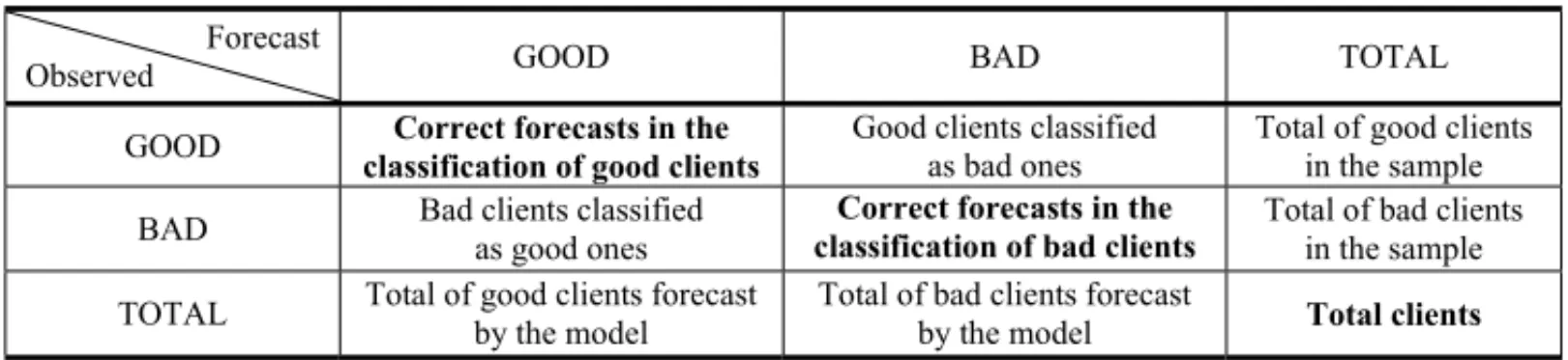
The percentage of correct classifications should be evaluated by crossing observed results and forecast results, as shown in Table 3. In the main diagonal are the cases correctly classified, bad clients who were forecast to be bad and good clients forecast as good. Thus, the rate of correct forecasting is measured by dividing the number of correctly classified clients by the total number of clients who were part of the analysis. Experts consider that models which have a correct forecast rate above 65% are satisfactory (Picininiet al., 2003).
Table 3– Verification of correct forecasts in the classifications of the model.
Forecast
Observed GOOD BAD TOTAL
GOOD Good clients classified as bad ones Total of good clients in the sample
BAD Bad clients classified as good ones
Total of bad clients in the sample
TOTAL Total of good clients forecast by the model
Total of bad clients forecast by the model
The KS test has the characteristic of simplicity. What is sought is to determine the maximum difference between two accumulated distributions. The two sub-populations (good and bad payers) translated by their respective results forecast by the model are displayed in cumulative distribution of frequencies. The differences between the distributions of good and bad payers for each forecast outcome are determined, and the value of the KS test is the greatest of these differences in module. If a difference greater than 30% is obtained, it can be considered that
the model is efficient in forecasting for the two groups (Picininiet al., 2003). The value can be
compared further with a critical value at 1% significance as per Equation 1:
K S1%=1.63 r
n1+n2 n1×n2
(1)
3.6 Steps towards implementation
In this last stage, the steps are suggested for implementing the model in the company: (i) pre-paring the information system; (ii) determining the cut-off point; (iii) recommendations and precautions when using the model; and (iv) reports on reviewing and monitoring the model.
By means of pre-defined criteria, the best model is chosen. Thereby the schedule for implemen-ting the model in the company should be drawn up. The companys Department of Information Technology should adapt their systems so as to receive the final model and to program its use in the areas involved (Gouvˆea & Gonc¸alves, 2006).
and the expected result of default for each level is calculated. A decrease in default is expected as the score increases. According to the author, the process of setting the cut-off point aims to seek the point at which the risk becomes so high that default becomes non-sustainable.
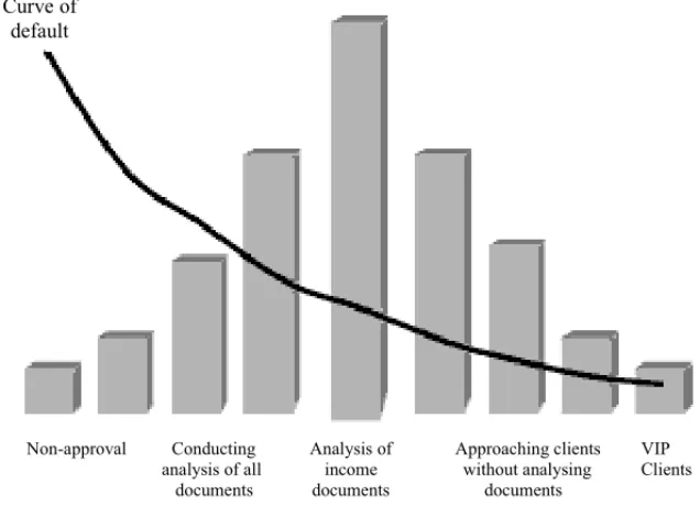
Besides identifying the behavior of default, the score obtained from the model can also be used to define ways of managing the granting of credit, as exemplified by Queiroz (2006). As can be seen in Figure 2, based on score ranges the author suggests some credit policies, such as: non-approval, conducting analysis of all the documents, analysis of income documents, approaching clients without analysing documents and VIP clients.
Curve of default
Non-approval Conducting Analysis of Approaching clients VIP analysis of all income without analysing Clients documents documents documents
Figure 2– Example of credit policy in accordance with default. Source: Queiroz (2006, p. 5).
One of the most important issues when implementing the model is to ensure that credit appli-cations are evaluated under the same assessment conditions used for the clients comprising the sample when the model was developed. It should therefore be ensured that information obtained at the time of analysing new proposals display similar conditions to those gathered at the model building period (Vasconcellos, 2004).
Pereiraet al.(2002) suggest that after using the model for a year, a review should be undertaken,
following the same steps as those used to build the original model. Thereafter, the authors state that a review is mandatory only if there is significant change in defaults, in profitability, in terms or conditions of business, and, especially, in the population profile. Such changes should be monitored through reports concerning model performance.
4 STUDY APPLIED
4.1 Description of the company, client and market
In conducting this research, information was used that came from a database of clients of a phar-macy network with branches throughout Rio Grande do Sul. This network itself offers clients a credit card to facilitate paying for purchases. So as to preserve the confidentiality of some information, some data were changed, which does not prevent the use and understanding of the proposed approach.
As the network under study currently has only one credit product, the target of the research is, therefore, the entire population of clients for this product. The card offered by the company can be used to pay for purchases made in the chain stores. Payment can also be made in up to three instalments, with a single due date for payment of the account sent to client´s address, which is similar to conventional credit card practice.
4.2 Information available and adjustment of the model to the case study
In accordance with the determination of the credit quality desired by the grantor, the definition of the groups of clients was arrived at according to the delays in payment in the period analyzed. For the company under study, the good client is defined as one who has not delayed payment or has delayed payments by up to 30 days, while bad clients are those who make payments with at least a delay of more than 60 days after payment due date.
The identification of the information available on company’s system, potentially useful as in-dependent variables for the analysis, was made based on the application that is completed by clients upon their requesting credit. At first, 16 variables were considered, including gender, age, marital status, level of education, profession, commercial and residential Zip Code, type of oc-cupation, type of residence, income, type of income, credit in other establishments, and payment of pension.
The sample period consisted of records of clients approved between December 2005 and June 2006. After the initial cleaning of the database during which incomplete or erroneous records were eliminated, the study sample had a total of 11,394 clients. Given that only the good clients and bad payers were used in order to construct the model, the sample comprises 6,305 good clients and 2,720 bad ones. With a view to constructing and validating the model, this set of data was divided into analysis and testing samples in the ratio of 80% and 20%, respectively.
4.3 Results obtained
Data modelling was performed using three rival models: discriminant analysis, logistic regres-sion and neural networks. To build the models using the techniques of discriminant analysis and logistic regression SPSS version 13.0 was used. The software used for training and testing the
neural networks, used to build the corresponding model wasBrainMaker Professional version
3.7. The stepwise estimation method was used with significance levels for the models input and output of variables of 5% and 10% respectively. Of the total of 69 dummy variables created, only 26 had a significant discriminatory power to compile the final discriminant model (Eq. 2), 29 for the logistic model (Eq. 3) and 26 for the neural networks model.
Y=0.154−1.172 DIDAD1−0.547 DIDAD23−0.315 DIDAD4+0.272 DIDAD6 +0.650 DIDAD7+0.933 DIDAD8+0.366 DSEXOF−0.344 DPRIM+0.257 DSUP+0.436 DCASADO+0.492 DTSERV67+0.641 DTSERV89−0.343 DFILHO−0.580 DRES ALU−0.602 DGCEPR12−0.329 DGCEPRE3−0.949 DGCEPCO1+0.298 DGCEPC56+0.707 DGCEPCO7−0.936 DGPROF1−0.399 DGPROF2+0.212
DGPROF5+0.293 DGPROF67−0.613 DCIDNA12−0.406 DCIDNA3+0.457 DCIDNA7 (2)
Y = 1
1+exp 0.876−0.829 DIDAD1−0.409 DIDAD23−0.252 DIDAD4+0.232 DIDAD6
+0.644 DIDAD7+1.047 DIDAD8+0.327 DSEXOF−0.287 DPRIM+0.270 DSUP
+0.410 DCASADO+0.340 DTSERV6+0.627 DTSERV7+0.792 DTSERV89−0.293 DFILHO−0.547 DRES ALU−0.392 DGCEPR12−0.172 DGCEPRE3+0.197 DGCEPRE5+0.328 DGCEPRE6+0.608 DGCEPRE7−0.768 DGCEPCO1+0.218 DGCEPC56+0.472 DGCEPCO7−0.718 DGPROF1−0.318 DGPROF2+0.283 DGPROF67−0.449 DCIDNA12−0.328 DCIDNA3+0.592 DCIDNA7)
(3)
To obtain the neural networks, non-recurring type MLP (Multilayer Percetron) networks were used, a function of sigmoid activation and the learning algorithm supervised by backpropagation of error, with only one hidden layer. Several networks were created with different numbers of hidden neurones in the hidden layer so as to check the performance regarding forecast of good and bad clients. The model with the best performance (with KS 40.3 for the sample analysis and 34.6 for the test sample) had 35 neurones in the hidden layer and was obtained after 1,200 rounds of the network.
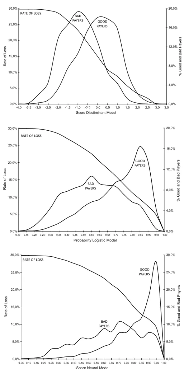
A joint assessment of the three models (discriminant, logistic and neural networks) is presented in Figure 3, with the distribution of the good and bad payers and the rate of loss, which corresponds to the percentage of bad payers over the total number of clients.
The two methods to check the forecasting power of the models were used: the percentage of correct classifications and the value of KS test. The results of the measurements for the three models are presented in Table 4. Both in the analysis sample and the test sample, the total per-centages of correct forecasts found for all three models are over 65% and the values for the KS test are greater than 30, the minimum values if a model is considered to have a good power of separation (Picininiet al., 2003).
Table 4– Performance measurements of the models built.
Percentage of correct
KS value classification
Model
Analysis Test Analysis Test sample sample sample sample Discriminant 73.2 72.1 36.7 30.7
Logistic 73.3 72.2 36.9 31.7
Neural 74.8 72.7 40.3 35.4
The three models built had satisfactory performances as to forecasting the clients as good and bad payers, as they obtained 73.2%, 73.3% and 74.8% correct classification with the techniques of discriminant analysis, logistic regression and neural networks, respectively. A small superiority of the neural networks over other techniques was observed, which is explained by its capability to incorporate non-linear effects and combining effects of the variables.
The neural network model had better separation in the forecast than the other two models, which is also verified by the higher value for the KS test (40.3). However, its programming in the companys system may be considered complex, which could lead the company to choose the implementation of either the discriminant model or the logistic model.
The results obtained from discriminant analysis and logistic regression were quite similar in terms of performance, also evidenced by the values of the KS test, 36.7 and 36.9, respectively. Thus, a choice between the two models would be given by means of analyzing the assumpti-ons for using the techniques, and, in this case, the logistic model has some advantages since it demands a smaller number of assumptions to be met.
5 CONCLUSIONS
The systematic presented in this study describes how to construct models for forecasting credit risk and addresses the definition of the population and details to be observed when selecting the sample and choosing the variables to be included in the credit risk model. The steps for prelimi-nary analyses of the data and building models using the three techniques chosen: discriminant analysis, logistic regression and neural networks were also presented. Lastly, the methods for choosing the best models and implementation steps for implementation in the companys system were discussed.
that the FCR model developed in this study can serve as a support tool for company resear-chers to build models adapted to specific business scenarios. A detailed comparison of the three techniques proposed here can be found in Selau (2008).
The use of models for credit risk forecasting eliminates the subjectivity of the analysis, by cre-ating a standardized decision-making procedure that can be complemented with extra pieces of information that are not contemplated in the mathematical model. Thus, it is possible to accele-rate credit analysis, which may allow an increase in business volume.
The systematic proposed in this paper was applied in a company that itself grants credit as a form of paying for its products. The application revealed that the systematic was useful for building and evaluating forecast models for credit risk. Using the proposed systematic, the most appropriate model can be identified, and the company can employ it as a tool to support the granting of credit by better selecting potential clients.
ACKNOWLEDGEMENTS
The authors would like to acknowledge the financial support provided by the Brazilian Research Supporting Agencies CAPES and CNPq.
REFERENCES
[1] ALMEIDAFC & DUMONTIER P. 1996. O uso de Redes Neurais em avaliac¸˜ao de riscos de ina-dimplˆencia.Revista de Administrac¸˜ao FEA/USP,31(1): 52–63.
[2] ANDREEVA, G, ANSELLAJ & CROOKJ. 2007. Modelling profitability using survival combination scores.European Journal of Operational Research,183(3): 1537–1549.
[3] ARMINGERG, ENACHE D & BONNE T. 1997. Analyzing Credit Risk Data: A Comparison of Logistic Discrimination, Classification Trees and Feedforward Networks.Computational Statistics,
12(2): 293–310.
[4] ASSAF NETO A & BRITO, G. 2005. Modelo de Classificac¸˜ao de Risco de Cr´edito de Grandes Empresas. In: Anais do V Congresso USP de Controladoria e Contabilidade, S˜ao Paulo – SP.
[5] BUENOVFF. 2003. Avaliac¸˜ao de risco na concess˜ao de cr´edito banc´ario para micros e pequenas empresas. Dissertac¸˜ao de Mestrado, PPGEP UFSC, Florian ´opolis.
[6] CAOUETTE JB, ALTMAN EI & NARAYANAN P. 1999. Gest˜ao do Risco de Cr´edito. O pr´oximo grande desafio financeiro. Qualitymark, S˜ao Paulo.
[7] CORRAR LJ, PAULO E & DIASFILHOJM. 2007. An´alise Multivariada: para cursos de Admi-nistrac¸˜ao, Ciˆencias Cont´abeis e Economia. Atlas, S˜ao Paulo.
[8] DESAI VS, CROOK JN & OVERSTREET JR GA. 1996. A comparison of neural networks and linear scoring models in the credit union environment.European Journal of Operational Research,
95(1): 24–37.
[10] GUIMARAES˜ IA & CHAVESNETOA. 2002. Reconhecimento de padr ˜oes: metodologias estat´ısticas em cr´edito ao consumidor.RAE Eletrˆonica EAESP/FGV,1(2): 1–14.
[11] HAIRJF, ANDERSONRE, TATHAMRL & BLACKWC. 2005. An´alise multivariada de dados. 5 ed. Bookman, Porto Alegre.
[12] HAYKIN S. 2001. Redes neurais: princ´ıpios e pr´atica. Trad. Paulo Martins Engel. 2 ed. Bookman, Porto Alegre.
[13] JOHNSONRA & WICHERNDW. 2002. Applied Multivariate Statistical Analysis. 5 ed. Prentice Hall, Upper Saddle River.
[14] LAWRENCED. 1992. Handbook of Consumer Lending. Prentice Hall, New Jersey.
[15] LEWISEM. 1992. An Introduction to Credit Scoring. Fair, Isaac and Co., Inc., San Rafael.
[16] MARQUESJM & LIMAJD. 2002. A Estat´ıstica Multivariada na An´alise Econˆomico-Financeira de Empresas.Revista FAE,5(3): 51–59.
[17] MENDES FILHOEF, CARVALHOACPLF & MATIASAB. 1996. Utilizac¸˜ao de redes neurais artifi-ciais na an´alise de risco de cr´edito a pessoas f´ısicas. In: Anais do III Simp ´osio Brasileiro de Redes Neurais, Recife – PE.
[18] MESTERLJ. 1997. What’s the Point of Credit Scoring? Business Review – Federal Reserve Bank of Philadelphia,4: 3–16.
[19] PEREIRASLG. 2006. Na mira do cr´edito.GV Executivo,5(1): 31-36, fev.-abr.
[20] PICININIR, OLIVEIRAGMB & MONTEIROLHA. 2003. Minerac¸˜ao de Crit´erio de Credit Scoring Utilizando Algoritmos Gen´eticos. In: Anais do VI Simp ´osio Brasileiro de Automac¸˜ao Inteligente, Bauru – SP.
[21] QUEIROZ RSB. 2006. A importˆancia dos modelos de Credit Scoring na concess˜ao de cr´edito ao consumidor no varejo. In: Anais do IX SEMEAD-FEA/USP, S˜ao Paulo – SP.
[22] SANTOSJ. 2000. An´alise de Cr´edito: Empresas e pessoas f´ısicas. Atlas, S˜ao Paulo.
[23] SCARPELRA & MILIONIAZ. 2002. Utilizac¸˜ao conjunta de modelagem econom´etrica e otimizac¸˜ao em decis˜oes de concess˜ao de cr´edito.Pesquisa Operacional,22(1): 61–72.
[24] SCHRICKELWK. 1997. An´alise de Cr´edito: concess˜ao e gerˆencia de empr´estimos. 3 ed. Atlas, S˜ao Paulo.
[25] SELAULPR. 2008. Construc¸˜ao de Modelos de Previs˜ao de Risco de Cr´edito. Dissertac¸˜ao de Mes-trado, PPGEP-UFRGS, Porto Alegre.
[26] SILVAJP. 2003. Gest˜ao e an´alise de risco de cr´edito. 4 ed. Atlas, S˜ao Paulo.
[27] SILVAJP. 2006. Os dois lados do cr´edito.GV Executivo,5(3): 68–72.
[28] SMITHM. 1996. Neural Networks for Statistical Modeling. International Thomson Computer Press, London.
[29] STEINERMTA, NIEVOLAJC, SOMA NY, SHIMIZU T & STEINERNETOPJ. 2007. Extrac¸˜ao de regras de classificac¸˜ao a partir de redes neurais para aux´ılio `a tomada de decis˜ao na concess˜ao de cr´edito banc´ario.Pesquisa Operacional,27(3): 407–426.