Braz. J. Chem. Eng. vol.31 número4

ISSN 0104-6632 Printed in Brazil

www.abeq.org.br/bjche

Vol. 31, No. 04, pp. 949 - 957, October - December, 2014 dx.doi.org/10.1590/0104-6632.20140314s00002857

Brazilian Journal

of Chemical

Engineering

CFD MODELING OF TWO IMMISCIBLE FLUIDS

MIXING IN A COMMERCIAL SCALE STATIC

MIXER

V. Abdolkarimi

*

and H. Ganji

Process & Equipment Technology Development Division, Research Institute of Petroleum Industry, (RIPI), Tehran, 1485733111, Iran.

Phone: (98 21) 48 25 24 97, Fax: (98 21) 44 73 97 13,

*_{E-mail: vabdolkarimi@gmail.com, Website: www.ripi.ir}

E-mail: Ganjih@ripi.ir

(Submitted: July 23, 2013 ; Revised: November 26, 2013 ; Accepted: December 24, 2013)

Abstract - A Computational Fluid Dynamics model based on the Eulerian formulation for multiphase flow was developed to model the mixing hydrodynamics of two immiscible fluids in a commercial scale static mixer. The two immiscible liquids were condensate and caustic solutions and were considered as two phases that are interpenetrating each other. The aim of this study was to develop a comprehensive Computational Fluid Dynamics model for predicting the impact of hydrodynamic parameters such as length, diameter and the arrangement of the corrugated plates of a static mixer on the degree of mixing and the pressure drop of the mixture. The model has been evaluated by comparing predictions of the degree of mixing and the mixture pressure drop with the same data available for the static mixer of the desulfurization plant of the Kharg petrochemical company. It has been shown that the predictions of the developed model are well adapted to the experimental data.

Keywords: CFD; Eulerian model; Static mixer; Hydrodynamics.

INTRODUCTION

Demercaptanization of condensate products (DMC) is widely used in the petroleum industry to remove COS, H2S, CS2 and mercaptans existing in

conden-sate products. There are different kinds of demer-captanizaton technologies with respect to the various amounts and kinds of mercaptans which are included in condensate products. The most complete demer-captanizaton technology is DMC-3. In this process, COS, H2S, CS2 and light mercaptans are removed from

condensate using 10 weight percent caustic solution. Caustic solution cannot extract heavy mercaptans. In this case, they are oxidized to disulphide in the pres-ence of enriched oxygen air (60 percent of oxygen by weight), caustic solution and IVKAZ catalyst. In

addition, for the separation of light mercaptans from caustic solution, the solution is oxidized over the IVKAZ catalyst. After oxidation, light mercaptans are converted to disulphide and separated from the caustic solution. The caustic which is recovered in the oxidation unit is sent to the extraction unit for extracting light mercaptans.

On the other hand, continuous mixing is used for mixing large amount of fluids and usually requires a complicated control system; hence it is more expen-sive than a batch procedure. The continuous method is especially used when direct delivering of blending products to consumers is required. In the continuous mixing method, a static mixer is used as the in line blending unit, which promotes the yield of the mix-ing process. The special geometry of a static mixer increases the mixing efficiency of fluids.

The main principles of static mixers are well de-scribed in the open literature (Grace, 1971; Cybulski and Werner, 1986; Mutsakis et al., 1986; Myers et al., 1997; Thakur et al., 2003). They may be used in order to carry out every mixing operation such as mixing of miscible fluids, heat transfer and thermal homogenization, or liquid–liquid dispersion, as well as gas–liquid dispersion. Static mixers offer advan-tages such as no moving parts, small space require-ments, little or no maintenance requirerequire-ments, many construction materials, narrow residence time distri-butions, enhanced heat transfer, and low power re-quirements. In fact, the only energy cost, represented by motionless mixers, comes from the external pump-ing power needed to propel materials through the mixer. That is why their use for continuous processes is an attractive alternative to classical agitation de-vices, since similar and sometimes better perform-ances can be achieved at a lower cost (Theron and Sauze, 2011).

If static mixers find many industrial applications for mixing of miscible liquids, there are few exam-ples of emulsification with static mixers. The most investigated mixer for liquid–liquid dispersion in turbulent flow in the literature is the classical Kenics helical mixer (Middleman, 1974; Chen and Libby, 1978; Haas, 1987; Berkman and Calabrese, 1988; Yamamoto, 2007). Emulsification, using the Sulzer SMX mixer, has been studied not only in laminar flow (Legrand et al., 2001; Das et al., 2005; Liu et al., 2005; Rama Rao et al., 2007; Fradette et al., 2007; Gingras et al., 2007) but also in turbulent regime (Streiff et al., 1997). Results for liquid–liquid disper-sion are also reported in the literature using the SMV mixer (Streiff, 1977).

With respect to the important role of the geomet-rical parameters of a static mixer, in this study we use CFD modeling as a powerful tool for evaluating the influence of geometrical parameters (such as length, diameter and pressure drop that are caused by special arrangement of static mixer planes) on mix-ing efficiency and the pressure drop of a commercial scale static mixer which is employed in the DMC unit of the Kharg petrochemical company.

INDUSTRIAL STATIC MIXER

For the mixing of low viscosity fluids, a special kind of static mixer such as the GV static mixer, made by the Stamix Company, is used. The GV static mixer is considered to be a high intensity design that creates a homogeneous mix in just a few pipe diameters. It is made of corrugated plates that are stacked on top of each other in an alternating-crossing fashion to form open intersecting channels that are at a 45°angle rela-tive to the pipe axis. Adjacent mixing elements are oriented 90° relative to each other to create 3-dimen-sional mixing (Figure 1). The “GV” static mixer is util-ized primarily in turbulent flow applications and cre-ates a very high degree of mixing in a short length. Typical applications include the mixing of low viscos-ity liquids, mixing of gases, gas-liquid contacting and immiscible liquid dispersion (www.stamixco.com).

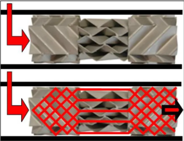
The GV static mixer continuously divides and re-combines the process streams to be mixed along the entire length of the mixing unit (Figure 2). In gas-liquid contacting and immiscible liquid dispersion applica-tions, the high shear field, created at each of the crossing points of adjacent corrugated plates, assures that intense mixing and contacting occurs over the entire volume of the mixer diameter and length. This generates small droplets/bubbles of a consistent size that are evenly distributed throughout the entire pipe diameter, resulting in high mass transfer rates.

The degree of mixing and the pressure drop per unit length of a mixer can be dialed in by varying the mixing element geometric parameters. This is ac-complished by varying the number of mixing layers (corrugated plates), corrugated plate angle relative to the pipe axis, mixing element L/D and the use of spacers between mixing elements to enhance homo-geneity with little pressure drop.

The standard GV mixing element consists of five corrugated plates. In applications where high degrees of mixing, short length and high shear are critical parameters, the overall mixer length can be short-ened by augmenting the number of mixing layers (corrugated plates, Figure 3).

The standard GV mixing element has a corru-gated layer angle of 45°relative to the pipe axis. In applications where low pressure drop is required, the angle is decreased to 30°, which dramatically lowers pressure drop.

Figure 1: GV static mixer with three mixing elements. Each mixing element has 5 corrugated plate mixing layers stacked at alternating 45°angles relative to the pipe axis.

Figure 2: Flow pattern through three GV mixing elements of 5 layer construction. Note that adjacent mixing elements are oriented 90°relative to each other.

Figure 3: Number of mixing layers (corrugated plates) in a specific pipe size.

The commercial scale static mixer of the Kharg petrochemical company has five corrugated plates in each mixing element that are aligned at the angle of 45°relative to the pipe axis. For each mixing ele-ment, the ratio of L/D is equal to unity. There are 6 mixing elements with spacers between them. The diameter and length of the static mixer are 10 inches and 3 meters, respectively. The geometry of the com-mercial static mixer is depicted in Figure 5 and the specifications are given in Table 1.

Figure 5: Geometry of the commercial static mixer.

Table 1: Specifications of commercial static mixer. Length of static mixer (m) 3 Diameter of static mixer (m) 0.254 Number of mixing elements 6 Length of mixing element (m) 0.254 Angle of mixing element corrugated plates (D) 45°

Number of spacers 3

Length of spacer (m) 0.254

COMPUTATIONAL MODEL

CFD modeling involves three main steps: (1) Creating the model geometry and grid. (2) Defining the appropriate physical models and (3) Defining the boundary and operating conditions. The governing con-servation equations of mass, momentum and physical models involved in the process are discretized over control volumes and solved by a finite volume method via the Fluent 6.3.3 commercial CFD toolbox. The whole volume of the static mixer is divided into 14 million tetrahedral control volumes. The mesh which is generated near the wall surfaces was refined to achieve the adequate y+ value (y+ < 300). The grid that is created on the surface of the corrugated plates is shown in Figure 6.

To solve the conservation equations, the fluid conditions at the inlet and outlet boundaries should be determined. Therefore, fluid conditions for con-densate and caustic solution are given in Table 2.

Figure 6: Triangular grids on the surface of the cor-rugated plates.

Table 2: Fluid conditions. Winter Case Run Case

Inlet Outlet Fluid name

Stabilized condensate

Caustic solution (10%)

Condensate + caustic Fluid quantity total

(kg/h) 209393.6 15098.2 224491.8

Liquid

(kg/h) 209393.6 15098.2 224491.8

Density

(kg/m3) 714.7 1103.9 728.9

Viscosity

(kg/(m.s)) 4.44E-4 9.5 E-4 5.5 E-4

Liquid

Surface Tension N/m

1.83 E-4 7.5 E-4 2.15 E-4

The two-phase flow equations are solved in the Eulerian framework that considers two fluids as a continuous phase that are penetrating each other. The contribution of each phase in the continuity and mo-mentum equations is attended by the volume fraction of each phase. This problem can be solved in steady state mode, but it is likely to lead to convergence problems; therefore, the unsteady state formulation is used. The time step size is selected as 0.001 seconds and the initial conditions are as follows:

Volume fraction of caustic solution = 0, Velocity of condensate = 0.5 m/s, Turbulent intensity of con-densate phase = 0.01. After 30 seconds the numerical solution approaches steady conditions.

The continuity equation for each phase is:

(

)

₍

₎

0

. =

∇ + ∂ ∂

q U q q t

q

qρ _{α ρ}

α

(1)

where Uq

JJG

is the velocity and αq is the volume

fraction of each phase.

(

) (

)

1

q q q q q q q

n

q q pq q q

p

U U U

t

P R g

α ρ α ρ

α τ α ρ

=

∂ _{+ ∇ =}

∂

− ∇ + ∇ +

∑

+

G G G

G (2)

where R_Pq is the fluid-fluid drag force. The subscripts 'p' and 'q' refer to the discrete phase of caustic and continuous phase of condensate, respectively.

(

P q

)

Pq Pq Pq

drag R U U

F _, = =β G − G (3)

where

β

_Pq is the fluid-fluid drag coefficient.

p p p q Pq f τ ρ α α

β = ₍₄₎

where

f

, the drag function, is defined differently for the different exchange-coefficient models and the

p

τ

"particulate relaxation time'' is defined as:

q p p p d μ ρ τ 18 2

= (5)

where dp is the diameter of the droplets of phase p.

For the model of Schiller and Naumann, (1935):

24 Re

D

C

f = (6)

1000 Re 0.44 1000 Re )/Re 0.15Re 24(1 0.687 ⎩ ⎨ ⎧ > ≤ + = D

C (7)

Re is the relative Reynolds number. The relative

Reynolds number for the primary phase k and

secondary phase p is obtained from:

q p q p

qU U d

μ ρ G − K =

Re (8)

Due to the high strain rate of fluid between corrugated plates, the Realizable k-e model is applied for modeling the effect of turbulence on flow field velocities (Shih et al., 1995).

(

)

(

)

,

,

. t q

q q q q q q

k

k q q q

k k U k

t

G

μ

ρ ρ μ

σ ρ ε ⎡⎛ ⎞ ⎤ ∂ _{+ ∇ = ∇ + ∇} ⎢⎜ ⎟ ⎥ ∂ _{⎣⎝ ⎠ ⎦} + − JJG (9)

(

)

(

)

, 2 .

q q q q q

t q q

q q q

k q q q

U t

C k

ρ ε ρ ε

μ ε

μ ε ε ρ

σ υ ε

∂ _{+ ∇} ∂ ⎛ ⎞ ⎡⎛ ⎞ ⎤ ⎜ ⎟ = ∇_⎢⎜ + _⎟∇ _⎥+ − ⎜ + ⎟ ⎝ ⎠ ⎣ ⎦ _{⎝ ⎠} JJG (10)

where σ_ε, σ_k are turbulent Prandtl numbers and μ_t,q is the turbulent viscosity.

q

k and ε_q are turbulent kinetic energy and dissipa-tion rate, respectively.

ε ρ

μt= C_μ k2 (11)

ε μ ∗ + = kU A A C S 0 1 (12) ij ijS S

U∗= (13)

φ

cos 6 A , 04 . 4 _S

0= =

A (14)

( )

1 1 cos 6 3 1 2

ij jk ki 3

j i

ij ij ij

i j

S S S W , W ,

S

U U

S S S , S

x x

ϕ₌ − ₌

⎛∂ ∂ ⎞ = = ⎜_⎜ + ⎟_⎟ ∂ ∂ ⎝ ⎠ (15)

RESULTS AND DISCUSSION

By using CFD modelling, we can estimate pre-cisely the velocity and volume fraction distribution of the caustic solution as the secondary phase and gas condensate as the primary phase. According to Table 2, the volume fraction of caustic at inlet would be 0.045 if caustic solution and condensate were mixed completely. At the inlet boundary, two phases enter separately for evaluating the performance of a commercial static mixer for mixing of two fluids. The entering face of the static mixer is divided into two semi-circles and phases which enter the mixer through the semi-circles separately at specified mass flow rates (Table 2). The Eulerian formulation of multiphase flow is used to describe the motion of each phase.

due to the existence of the corrugated plates, makes it essential to use a proper turbulent model that can evaluate the velocity field for both fluids correctly. Hence, the realizable k-e model was selected to predict turbulent flow field velocities. The purpose of using a static mixer is perfect mixing of fluids, which is obtained by dividing flow streams, radial mixing and vortex creation in a static mixer. The flow patterns of condensate can be recognized from the velocity vectors.

(a)

(b)

(c)

Figure 7: The velocity vectors of condensate (m/s) at the (a) inlet, (b) middle, (c) outlet of the static mixer on a longitudinal section.

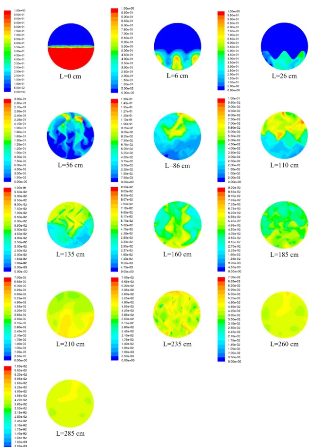
In Figure 8, the contours of condensate volume fraction at (a) the inlet (b) the middle of mixer and (c) the end of static mixer are shown. As is obvious, at the inlet of static mixer two fluids enter separately from two inlet boundaries and then, after crossing the corrugated plates, the direction of flow changes dramatically. This direction change leads to mixing of fluids, which is completed at the end of the mixer.

(a)

(b)

(c)

Figure 8: The volume fraction contours of conden-sate at the (a) inlet, (b) middle, and (c) outlet of the static mixer on a longitudinal section.

L=26 cm L=6 cm

L=0 cm

L=110 cm L=86 cm

L=56 cm

L=185 cm L=160 cm

L=135 cm

L=260 cm L=235 cm

L=210 cm

L=285 cm

simulated results in Figure 11. Mixture density was calculated according to the averaged caustic volume fraction along the mixer (Figure 10), which is calcu-lated on the cross-sectional planes (Figure 9). As can be seen from Figure 11, there is a great amount of difference between measured and calculated mixture density. This is because of the location of the meas-uring probe, which is in the vicinity of the conden-sate phase, but the calculated mixture density is based on the averaged caustic volume fraction over each cross-sectional plane.

Figure 10: The area weighted average of caustic volume fraction over cross-sectional planes along the static mixer

Figure 11: The comparison between predicted and experimental mixture density values at various cross-sectional planes

According to the fact that the most important pa-rameter in designing a static mixer is the mixer’s

pressure drop, the pressure drop of the mixture along the commercial static mixer is shown in Figure 12. According to CFD modeling, the total pressure drop of the mixture through the static mixer is 20 kPa, which is in good agreement with experimental and design data (actual pressure drop = 25 kPa, allowable pressure drop = 50 kPa). In Figure 12, there are three regions along the static mixer axis (Z = 0.25m, Z = 0.75m, Z = 1.5m) where the static pressure of the mixture increases slowly. These regions are relevant to spacers where the corrugated plates do not exist.

Figure 12: Mixture pressure drop versus axial posi-tion through a commercial scale static mixer.

CONCLUSIONS

gradually after decreasing by passing across mixing element plates and recovers somewhat the flow static pressure.

REFERENCES

Berkman, P. D. and Calabrese, R. V., Dispersion of viscous liquids by turbulent flow in a static mixer. AIChE J., 34, 602-609 (1988).

Chen, S. J. and Libby, D. R., Gas–liquid and liquid– liquid dispersions in a Kenics mixer. In: 71st An-nual AIChE Meeting (1978).

Cybulski, A. and Werner, K., Static mixers-criteria for applications and selection. Int. Chem. Eng., 26, 171-180 (1986).

Das, P. K., Legrand, J., Morançais, P. and Carnelle, G., Drop breakage model in static mixers at low and intermediate Reynolds number. Chem. Eng. Sci., 60, 231-238 (2005).

Fradette, L., Tanguy, P., Li, H. Z. and Choplin, L., Liquid liquid viscous dispersions with a SMX static mixer. Trans. IChemE, 85, 395-405 (2007). Gingras, J. P., Fradette, L., Tanguy, P. and Bousquet,

J., Inline bitumen emulsification using static mix-ers. Ind. Eng. Chem. Res., 46, 2618-2627 (2007). Grace, C. D., Static mixing and heat transfer. Chem.

Proc. Eng., 57-59 (1971).

GV Static mixer product bulletin homepage. [Online]. Available at: <http://www.stamixco.com>. (Ac-cessed: October 15, 2013).

Haas, P. A., Turbulent dispersion of aqueous drop in organic liquids. AIChE J, 33, 987-995 (1987). Legrand, J., Morançais, P. and Carnelle, J., Liquid

liquid dispersion in an SMX Sulzer static mixer Trans. IChemE, 79, 949-956 (2001).

Liu, S., Hrymak, A. N. and Wood, P. E., Drop break up in an SMX static mixer in laminar flow. Can. J. Chem. Eng., 83, 793-807 (2005).

Middleman, S., Drop size distributions produced by

turbulent pipe flow of immiscible fluids through a static mixer. Ind. Eng. Chem. Process. Des. De-velop, 13, 78-83 (1974).

Mutsakis, M., Streiff, F. and Schneider, G., Advances in static mixing technology. Chem. Eng. Prog., 42-48 (1986).

Myers, K. J., Bakker, A. and Ryan, D., Avoid agita-tion by selecting static mixers. Chem. Eng. Prog., 28-38 (1997).

Rama Rao, N. V., Baird, M. H. I., Hrymak, A. N. and Wood, P. E., Dispersion of high- viscosity liquid liquid systems by flow through SMX static mixer elements. Chem. Eng. Sci., 62, 6885-6896 (2007).

Schiller, L. and Naumann, Z., A drag coefficient correlation. Ver. Deutsch. Ing., 77-318 (1935). Shih, T. H., Liou, W. W., Shabbir, A., Yang, Z. and

Zhu, J., A new k-e eddy-viscosity model for high Reynolds number turbulent flows - model develop-ment and validation. Computers Fluids, 24(3), 227-238 (1995).

Streiff, F. A., Mathys, P. and Fischer, T. U., New fundamentals for liquid liquid dispersion using static mixers. Récents Prog. Génie Procédés, 11, 307-314 (1997).

Streiff, F. A., In-line dispersion and mass transfer using static mixing equipment. Sulzer Techn. Rev., 108, 113 (1977).

Thakur, R. K., Vial, K. D. P., Nauman, E. B. and Djelveh, G., Static mixers in the process industries – a review. Trans. IChemE, 81, 787-826 (2003). Theron, F. and Le Sauze, N., Comparison between

three static mixers for emulsification in turbulent flow. International Journal of Multiphase Flow, 37(5), 488-500 (2011).