qCube: Efficient Integration of Range Query
Operators over a High Dimension Data Cube
Rodrigo Rocha Silva1,3
, Joubert de Castro Lima2
, Celso Massaki Hirata1
1
ITA - Instituto Tecnológico de Aeronáutica
2
UFOP - Universidade Federal de Ouro Preto
3
FATEC - Faculdade de Tecnologia de Mogi das Cruzes
{rrochas, hiratacm, joubertlima}@gmail.com
Abstract. Many decision support tasks involve range query operators such as Similar, Not Equal, Between, Greater or Less than and Some. Traditional cube approaches only use Equal operator in their summarized queries. Recent cube approaches implement range query operators, but they suffer from dimensionality problem, where a linear dimension increase consumes exponential storage space and runtime. Frag-Cubing and its extension, using bitmap index, are the most promising sequential solutions for high dimension data cubes, but they implement only Equal and Sub-cube query operators. In this paper, we implement a new high dimension sequential range cube approach, named Range Query Cube or justqCube. The qCube implements Equal, Not Equal, Distinct, Sub-cube, Greater or Less than, Some, Between, Similar and Top-k Similar query operators over a high dimension data cube. Comparative tests with
qCubeand Frag-Cubing use relations with 20, 30 or 60 dimensions, 5k distinct values on each dimension and 10 million tuples. In general,qCubehas similar behavior when compared with Frag-Cubing, but it is faster to answer point and inquire queries. Frag-Cubing could not answer inquire queries with more than two Sub-cube operators in a relation with 30 dimensions, 5k cardinality and 10M tuples. In addition,qCube efficiently answered inquire queries from such a relation using six Sub-cube or Distinct operators. In general, complex queries with 30 operators, combining point, range and inquire operators, took less than 10 seconds to be answered byqCube. A massiveqCubewith 60 dimensions, 5k cardinality on each dimension and 100M tuples answered queries with five range operators, ten point operators and one inquire operator in less than 2 minutes.
Categories and Subject Descriptors: H.2 [Multidimensional and Temporal Databases]: Miscellaneous; H.3 [Query Processing and Optimization]: Miscellaneous; I.7 [Big Data]: Miscellaneous
Keywords: data cube, high dimension, inquire query, OLAP, range query
1. INTRODUCTION
Data Cube relational operator [Gray et al. 1997] pre-computes and stores multi-dimensional aggrega-tions, enabling users to perform multi-dimensional analysis on the fly. A data cube has exponential storage and runtime complexity according to a linear dimension increase. It is a generalization of the group-by relational operator over all possible combinations of dimensions with various granularity aggregates [Han 2011]. Each group-by, called acuboid or view, corresponds to a set of cells described astuples over thecuboid dimensions.
A data cube has base cells and aggregate cells. Suppose there is data cube with 3 dimensions. Let us consider a tuple t1 = (A1, B1, C1, m) of a relation, where A1, B1, C1andAn, are dimension
attributes and m is a numerical value representing a measure of t1. Given t1, in our example, a
data cube has seven tuples representing all possible t1 aggregations, and they are: t2(A1, B1,∗, m),
t2 = (A1,∗, C1, m), t4 = (∗, B1, C1, m), t5 = (A1,∗,∗, m), t6 = (∗, B1,∗, m), t7 = (∗,∗, C1, m),
This work was partially supported by ITA, UFOP, FATEC-MC and by FAPESP under grant No. 2012/04260-4 provided to the authors.
t8= (∗,∗,∗, m), where "*" is a wildcard representing all values of a cube dimension.
Generally speaking, a cube, computed from relationABC with cardinalitiesCA, CB andCC, can
have23or(C
A+ 1)x(CB+ 1)x(CC+ 1)tuples. Our cube has three dimensions with equal cardinality
CA = CB = CC = 1. If we want to select some values and not all (*) values, data cube problem
becomes even harder. We can choose, for example, a range of continuous dimension values or some categorical values, drastically increasing the number of tuples in this new cube, called Range Cube
(RC).
Let us consider relationABC with cardinalities CA, CB and CC equal to 2. This small relation
can have eight tuples of type ABC, but twenty seven tuples in a full data cube. If we introduce a new wildcard "**", representing two attributes of the same dimension, we have new tuples, such as: t28= (A1A2, B1, C1, m1), t29 = (A1, B1B2, C1, m2), t30= (A1, B1B2, C1C2, m3)and many others.
Tuplest28, t29andt30measures represent new summarized values. In general, these approaches answer
queries similar to: "find the total sales for customers with age from 35 to 50, in year 1998-2008, in area L and with auto insurance". Instead of (CA+ 1)x(CB+ 1)x(CC+ 1)tuples in the cube, computed
from relation ABC, a range cube RC can have 2CAx2CBx2CC tuples. In our example, RC has
22x22x22= 64tuples from a relationABC with 8 tuples.
It is impracticable to compute all those tuples, so there are many data cube indexing strategies to reduce query response time without drastically increasing both computation runtime and storage [Chun et al. 2004; Lee et al. 2000; Liang et al. 2000; Ho et al. 1997]. Usually, these approaches answer range cube queries with COUNT, MIN, MAX and SUM measure functions.
The dimension increase also makes cube combinatorial problem harder. If instead of relationABC, we consider relation ABCD and CA =CB =CC =CD = 2, we can have 16 tuples of type ABCD,
81 tuples in a full data cube and 256 tuples in aRC. Most of cube approaches are not designed for high dimension data cubes; and in particular,RC approaches cannot compute high dimension data cubes. Cubing [Li et al. 2004] is the first efficient high dimension data cube solution. Frag-Cubing implements an inverted index of tuples, i.e., each tuple attribute is associated with 1-n tuple identifiers. Point queries with two or more attributes are answered by intersecting tuple identifiers from attributes. Unfortunately, Frag-Cubing only implements Equal and Sub-cube query operators. There is a proposal [Leng et al. 2006] to implement a bitmap index approach [Chan and Ioannidis 1998] to address a solution to the dimensionality problem; however the approach cannot compute data cubes with both high cardinality and tuples. No range and inquire query operators were implemented.
In this paper, we propose a new cube approach, named Range Query Cube or justqCube, which implementsEqual, Not Equal, Greater orLess than, Some, BetweenandSimilarrange query operators andDistinct, Sub-cube and Top-k Similar inquire query operators over a high dimension data cube. TheqCube approach implements a set of tuple identifiers per dimension attribute, similar to Frag-Cubing, so thatqCubecan answer point queries using tuple identifiers intersections and range queries using unions plus intersections algorithms, regardless measure function types. Tests with a 10 million tuple relation demonstrated thatqCube can answer sequentially multiple point, range and inquire query operators in a single query with 30 attributes in less than 10 seconds. A massive qCube
with 60 dimensions, 5k cardinality and 100M tuples answered queries with 5 range operators, 10 point operators and 1 inquire operator in less than 2 minutes, without multicore or multicomputer high performance architectures benefits. qCube is a promising alternative to efficiently answer high dimension range queries from massive relations.
The rest of the paper is organized as follows: Section 2 details Frag-Cubing and a bitmap cube solution, as well as some promising range query approaches, pointing out their benefits and limitations. Section 3 details qCube approach, i.e., its architecture and algorithms. Section 4 describes the
2. RELATED WORK
There are several cube approaches, but only two of them implement a sequential high dimension cube solution. Frag-Cubing [Li et al. 2004; Leng et al. 2006] implement a partial cube approach using in-verted index and bitmap index, respectively. Data cube operator has storage and runtime exponential complexity according to a linear dimension increase. Li et al. [2004] illustrate the exponential storage impact of different cube approaches using only 12 dimensions. There is a clear curve saturation in using Full, Iceberg, Dwarf, MCG, Closed or Quotient approaches [Brahmi et al. 2012; Ruggieri et al. 2010; Lima and Hirata 2011; Xin et al. 2006; Sismanis et al. 2002] for cubes with 20, 50 or 100 dimensions.
Frag-Cubing implements the inverted tuple concept, i.e., each inverted tupleiT has a dimension attribute, a list of tuple identifiers and a corresponding list of measures. For instance, three tu-ples: t1 = (tid1, a1, b2, c2, m1), t2 = (tid2, a1, b3, c3, m2) and t3 = (tid3, a1, b4, c4, m3) produce the
inverted tuple iT a1 = (a1, tid1, tid2, tid3, m1, m2, m3), where the attribute a1 is found at a
rela-tion with identifiers tid1, tid2 and tid3, and tid1 has measure value m1, tid2 has measure value m2
and tid3 has measure value m3. Suppose a new tuple t4 = (a1, b4, c1, m4) with the inverted tuple
iTb4 = (b4, tid3, tid4, m3, m4). A query q = (a1, b4, COU N T) can be answered by iTa1 ∩iTb4 =
(a1b4, tid1, COU N T(m1))- whereiTa1∩iTb4 means the set that contains all those elements thatiTa1
andiTb4 have in common.
The intersection complexity is proportional to the tuple with the smallest set of identifiers. In our example, iTb4 with two tuple identifiers is the smallest set, soiTb4∩iTa1 is more efficient than
iTa1∩iTb4. The number of tuple identifiers associated per dimension attribute can be huge, therefore
relations with low cardinality dimensions and high number of tuples produce costly set intersections. As the sets of tuple identifiers become smaller, Frag-Cubing query becomes faster, so relations with low skew and high cardinalities and dimensions are more suitable to be computed by using Frag-Cubing andqCubeapproaches.
Fangling et al. [2006] replace the inverted index with a bitmap index. Each dimension attributeat has a set of bitsB, indicating whether at is found or not at each tuple. There is a clear limitation in the number of tuples as B becomes greater. The authors propose a compact index, eliminating zeros and ones sequences fromB, but their approach is useful only for small relations. The cardinality imposes a new hard problem, since for each new dimension attributeat’, a new set of bitsB’ must be created with size equal to the number of tuples. Relations with thousands of different attributes per dimension and hundred millions of tuples cannot be efficiently computed using bitmap index, even if it is not a high dimension relation.
Data cube range query was first addressed by using a multidimensional array solution [Ho et al. 1997]. For a data cube withD dimensions andC cardinality at each dimension, there are(C+ 1)D
cells to represent a data cube, where each array cell has a 32-64 bit measure value. A second array of cells of the same size is used to store the prefix-sum values, so storage and runtime costs to update the data cube become a bottleneck. A relation with lots of empty cells is not rare, therefore there are improvements to reduce empty cells and update costs [Liang et al. 2000; Chun et al. 2004], but even these compact prefix-cube approaches are not efficient to compute text and temporal dimen-sions, where cardinalities cannot be defineda priori. Their best results have range query complexity O(CD/6), where
C is a dimension cardinality andD is the number of query dimensions, so they are not designed for high dimension data cube range queries, whereD is greater than 30-50 dimensions.
3. THE QCUBE APPROACH
Fig. 1. qCube architecture.
The qCubeComputation component is responsible for reading the entire base relation with D
dimensions and creating a map of tuple identifiers (TIDs) per relation attribute. Each map has an attribute as a key and a set of TIDs as a value. This way,qCubeComputation creates all inverted tuples ofqCubeapproach. In the example above, there are dimensionsA, B . . . nand each dimension has a set of attributes. DimensionA has, for example,(a1, a2. . . an) attributes. TheqCubeQuery
component receives a user query, executes intersections, unions and sorting algorithms using TIDs, and producesqCuberesults. BeforeqRis produced, the final set of TIDs, generated byqCubeQuery
component, is processed byqMeasureProcesscomponent, which collects measure values using TIDs and performs statistical computation with such values.
All TIDs generated from a base relation must fit in main memory. User queries, including point, range and inquire queries, are answered byqCubeQuery component sequentially. External memory and parallelqCubeversions, including multicore and multicomputer, are part of future improvements.
3.1 qCubeComputation Algorithm
A relationR is a set of tuples, where each tuple t is defined ast = (T ID, D1, D2. . . Dn). In t, nis
the number of dimensions,D is a specific dimension defined asDi = (ati1+ati2. . . atin), and ati is
an attribute of dimensionDi. The symbol ’+’ means a logical OR. The TID attribute is a unique
identifier, so there is no equal tuple in a relation.
GivenR and aqCubeComputation algorithmCA, the output is a data cubeqC = (. . .(iT ati1,
iT ati2. . . iT atin). . . im1, im2. . . imx), where each internal element (iT ati1, iT ati2. . . iT atin) of qC
represents a set of inverted tuples of a specific dimension. Each iT at, defined as iT at = (atij,
T id1. . . T idp), represents thejthinverted tuple of a dimension with indexi. The inverted tupleiT at
has an attribute valueati and a set of tuple identifiers(T id1. . . T idp)with sizep. Data cubeqC also
has(im1. . . imx), where eachim, defined asim= (T ID, mv), is an inverted measure composed by a
tuple identifier TID and a numeric measure valuemv. The computation algorithm proceeds as shown in Figure 2.
In the algorithm of Figure 2, variable sortedC stores dimension cardinalities to improve query response time. TheinvertedT is the main variable, storing all attributes of relation Rand their set of tuple identifiers TIDs. InvertedM stores all measures of relation R. For each tuple ofR, there are one or more entries ininvertedM maps. Basically, the algorithm computes dimension attributes (lines 7-9) and measure values (lines 11-14). We use an example of a relation with five dimensions in Table 1.1 to explain the basic idea of the algorithm. Each tuple of a relation is read and inverted, i.e. the first tuple of the input relation a1, b1, c1, d1, e1 is inverted, creating five new inverted tuplesa1T id1,
Fig. 2. qCube Computation algorithm.
Table I. A qCube example with five dimensions.
T id1, as Table 1.3 shows. The same occurs to the remaining tuples. After a complete relation scan,
all inverted tuples have been created, as Table 1.2 illustrates. The attributee2, for instance, occurs
four times in the relation;a1, b1, d1 andd2 occur three times. TheinvertedM variable is represented
by Table 1.3.
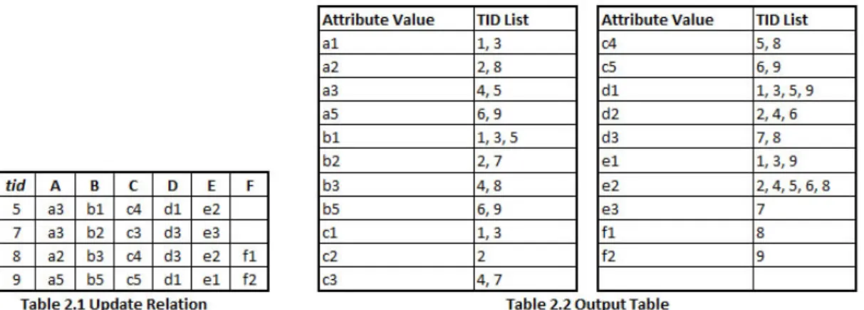
Table II. A qCube update example.
3.2 Update Algorithm
There are four types of updates: (i) new tuples can be added; (ii) attributes ofRcan be fused; (iii) new dimensions and measures can be added toR; (iv) dimension hierarchies can be reorganized. Data cube partition based on inverted tuples is very efficient for these types of updates. Dimension hierarchies rearrangements do not affectqC. New tuples can be added by calling the same computation algorithm. New dimensions can be computed without reprocessing the previous ones. The same occurs with new measures, which can also be associated with TIDs. An attribute fusion generates a new attribute at’ in R, where at’ is the union of two or more previous attributes. This way, qCube implements attribute fusion by uniting inverted tuple TIDs from two or more attribute values ofR.
Tables 2.1 and 2.2 illustrate the impact of update type (iii) inqCube. A new relation with six and not five dimensions must be computed andqCube does not require re-computations. In general, just new attributes and TIDs are inserted on qCube representation, as Table 2.2 illustrates. Table 2.2 considers Table 1.2 inverted tuples to illustrate a single update type. The remaining update types are trivial inqCube, thus they are not explained in this paper. Many cube approaches are not designed for these four update types, demanding in almost all cases a full cube reconstruction.
TheqCube approach adopts complementary arrays with small size. Map data structures encapsu-late multiple arrays, so there are more resizing operations, but fewer empty array cells. Furthermore,
qCube data access continues constant. Due to these cube representation properties, qCube can be extended to text cubes with few adaptations.
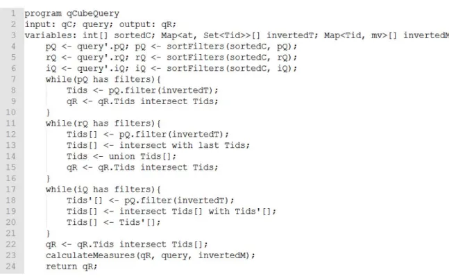
3.3 Query Algorithm
User queries of type Q are partitioned and classified by qCube into: (i) point query; (ii) range query and (iii) inquire query. From a query Q, qCube generates three other sub-queries pQ, rQ
andiQ, where pQ ∈Qis a set of Equal operators filtering different dimensions, rQ∈Q is a set of range operators filtering different dimensions, andiQ∈Qis a set ofpsize inquire operators filtering combinatorial results from different dimensions. A range-operator can be defined as rOp= (greater than + less than + between + some + different + similar x (f v1. . . f vn)). An inquire-operator iOp
can be defined asiOp =(sub-cube + distinct + top-k similar x(f v1. . . f vn)). The symbol ’+’ means
the logical OR and ’x’ means the logical AND. Range and inquire operators must have their types and a set of filter values, so in previous definitions ofrOpandiOp,(f v1. . . f vn)are filter values. Note
Fig. 3. qCube query algorithm.
In order to explain the query algorithm, we use an example. Suppose we have to answer the following queryQ:"What is the women journal research papers variance impact, using months 1, 3, 5, 7, 11, year 2012 and ages varying from 25-40 years? Return results for each country".
Algorithm in Figure 3 illustrates qCube query component. In line 4, point queries are returned from a query. InQ, they are (sex = women, paperType=journal, year=2012). A cardinality based sorting is executed to rearrange sex, paperType and year dimensions. The same occurs with range and inquire queries (lines 5 and 6). The range queries(month = (1,3,5,7,11), age <>25-40) are also sorted according to their cardinalities. InQ, there is inquire query(country=distinct).
While Q has point queries, an intersection is performed between current partial result qR and TIDs returned frominvertedM variable (lines 8 and 9). Dimensions sex, paperType and year require two intersections to conclude point query portion ofQ. While Q has range queries, each attribute TIDs returned from a rOp operator is intersected with point query TIDs (line 13). The results are united to produce another partial result. In our example, operatorrOp_Some =(1,3,5,7,11) has five intersections with TIDs of ((sex = women)∩(paperT ype = journal)∩(year = 2012)). Five results are united to produce partial result up to dimension month. The same occurs with operator between at age dimension.
Finally, lines 18-20 illustrate how to generate combinatorial results from sub-cube filter. Distinct and top-k similar filters are similar to this block of code. In our example, partial result TIDs must be intersected with all countries in the world. Line 23 summarizes an instruction to both retrieve numeric values frominvertedM variable of Algorithm 2 and perform statistical computation according to different measure functions (SUM, MAX, MIN, AVG, VARIANCE, RANK and many others).
and many others. Note that,Q can have no pQ on it. The same for rQ or iQ. This way, qCube
enables the end user to combine point, range and inquire queries. TheqCubeapproach adopts Apache library for statistical calculus.
In ann-dimensional data cube(D1, D2, . . . , Dn), a point querypQis in the form of{a1, a2, . . . , an:
M}, where eachaispecifies a value for dimensionDi andM is the inquired measure. ApQreceives a
data cubeqC and performs an efficient filterF on it. The filterF can be defined asF = (eq1∩eq2∩
. . .∩eqd), where eqi is theith EQUAL operator of F applied to dimension i of qC. Only EQUAL
operators are used in point queries. Each eqi EQUAL operator returns a set of tuple identifiers
(TIDs) from dimension i, so in general F is computed by successive intersections of all TID sets. Query response times can be improved by a sortedF, where dimensions with high cardinalities are intersected first. Dimensions with high cardinality normally produce attribute values with small sets of TIDs, therefore we can reduce intersection complexity. The variable sortedC in Algorithm in Figure 3 is used to rearrangepQ execution. F is incrementally computed, therefore there is a final optimization, where two sets of TIDs are previously compared to verify which one is the first set in the intersection. This way,qCube reduces even more the number of comparisons inpQ.
A range query applies an aggregation operation over all selected cells of an OLAP data cube where the selection is specified by providing ranges of values for numeric dimensions. ARange Query (rQ): Receives a data cube qC and performs a second filter F’ on it. The TIDs of pQ are intersected with TIDs ofrQ. The filterF’ can be defined asF’= (rOp1∩rOp2∩. . .∩rOpd), whererOpi is the
ith RANGE operator ofF’ applied to dimensioni of qC. F and F’ filter different dimensions. As
mentioned before,rOp can be classified into(greater than + less than + between + some + different + similar). EachrOpi RANGE operator returns a set of tuple identifiers (TIDs) from dimension i,
so in generalF’ is also computed by successive intersections of all TID sets.
Different frompQ, arQ filterF’has many intersection operations and a final union. More precisely, let’s userOpb, short forrOp operatorbetween, to illustrate the algorithm idea. Initially, one or more
attributes of a dimension are returned from filterrOpb. InvertedT variable in Algorithm in Figure
3 is used to perform C intersections withpQ TIDs and all attributes of rOpb TIDs before a final
union of C sets. C indicates all attributes that satisfy rOpb filter. The new attribute with these
TIDs is intersected with a second RI’ result. Therefore, successive multi-intersections-union cycles occur untilrQ has arOpto execute. The number of TIDs on each set is smaller if intersections occur before a union operation. The opposite idea is to first unite TIDs ofC dimension attributes and then intersect with pQ. This way, there are C union operations plus a larger TID set to be intersected withpQ. Experiments withqCube confirm this assumption.
Inquire Query(iQ) seeks for a set of cuboid cells inqC. It is a CPU bound operation, since it is a combinatorial problem. In ann-dimensional data cube(D1, D2. . . , Dn), an inquire query is in the
form of{a1, a2, . . . , an :M}, where at least oneai is marked as iQ to denote that dimension Di is
inquired.
AniQ operator receives a data cubeqC and performs a third filterF" on it. The TIDs ofiQ are intersected with TIDs of(pQ∩rQ). The filterF"can be defined asF” = (iOp1∩iOp2∩. . .∩iOpd),
where iOpi is the ith INQUIRE operator ofF" applied to dimension iof qC.F, F’ and F" filter
different dimensions. TheiOpoperators can be classified into(sub-cube + distinct + top-k similar). A sub-cube of one dimension is composed of all attributes of a dimension plus the summarized attribute all (*), the last indicating a measure value of a dimension and not one of its attributes. For each attribute of dimension i, there is a set of TIDs. TIDs from (pQ∩rQ) are intersected with each attribute TIDs of dimension i, forming a set of results. There areQsci=1(Ci+ 1) results whenQ has SC sub-cube filters in F". Ci indicates the cardinality of dimension i and SC is the number of
sub-cube filters.
of inquired dimensions is 0. On the other extreme, a full-cube query is a sub-cube query where the number of instantiated dimensions is d, where d is the number of dimensions [Li et al. 2004].
Distinct and sub-cube filters are identical for one dimension. Two or more dimensions increase the number of distinct results toQdisi=1Ci intersections with TIDs of(pQ∩rQ). It is also a costly
operation. Finally, the top-k similar filter selects only similar dimension attributes, thus it often has fewer combinations when compared with sub-cube or distinct operators. Unfortunately, there is a costly edit distance method, similar to that on the work of Ho et al. [1997], to select top-k attributes for each dimension.
Roll upoperations can be performed by attribute removal, therefore part of a new rolled upQ’
must be reprocessed. In our example, if user decides to roll up dimension age and consider all ages, the partial TIDs result computed up to dimension month is preserved. In our example, intersections with all countries in the world must be redone to buildQ’, sinceQ⊂Q′.
Drill-downis the reverse of roll-up. It navigates from less detailed data to more detailed data. Drill-down can be performed either by stepping down a concept hierarchy for a dimension or intro-ducing additional dimensions. Drill down on query Q always includes filter on it, therefore qCube
intersects the current resultqRwith one or more TIDs from the new filter. In a drill down scenario Q′ ⊂Q, whereQ’ is a drilled query fromQ. TheqCubeapproach implements drill down and roll up checking in successive user queries to reduce response times, since users frequently explore dimension hierarchies.
4. EXPERIMENTS
A comprehensive performance study was conducted to check the efficiency and the scalability of the proposed approach. We tested qCube Computation and Query algorithms against Frag-Cubing al-gorithm used by Li et al. [2004]. The qCube algorithms were coded in Java 64 bits (version 7.0). Frag-Cubing is a free and open sourceC++
application (http://illimine.cs.uiuc.edu/). In all exper-iments the relation can fit in main memory. Cube computation tests include both I/O and CPU times. I/O times are considered to load input relations from external memory to main memory. No swap operations are implemented in qCube and Frag-Cubing during a cube query or computation experiment. Only sequential versions are implemented. We ran the algorithms in two Intel Xeon six-core processors with 2.4GHz each core, 12MB cache and 128GB of RAM DDR3 1333MHz. There are seven disks SAS 15k rpm with 64MB cache each. The system runs Windows Server 2008 64 bits, High Performance version. All tests are executed five times, we remove the lowest/highest runtimes and an average is calculated for the three remaining runtimes.
For the remainder of this section, D is the number of dimensions, C is the cardinality of each dimension, T is the number of tuples in a base relation and S is the data skew. Skewness is a measure of the degree of asymmetry of a distribution. WhenS is equal to 0, data is uniform; as S increases, data becomes more skewed. Real databases are often skewed. The synthetic base relations were created using data generator provided by the IlliMine project. The IlliMine project is an open-source project to provide various approaches for data mining and machine learning. Frag-Cubing approach is part of IlliMine project.
4.1 Performance Evaluation of Point Queries and Skewed Relations
In the first experiment, we evaluate point queries according to the number of operators. Basically, we increase the number of EQUAL (eq) operators in a query. Tests use relations withS=0 and 2.5,D=30, 107
Fig. 4. Response time per query over 100 trials: T= 107
;C= 5000;D= 30;S= 0.
Fig. 5. Response time per query over 100 trials: T= 107
;C= 5000;D= 30;S= 2
.5.
of EQUAL operators increases, intersection costs dominate query response time, so the differences between Frag andqCube become proportional. Figure 4 illustrates a relation with moderate sized TID sets, thus query response time with six operators is faster in a uniform relation (Figure 4) than in skewed ones (Figure 5). In all point queries, using skewed or uniform relations,qCube is faster than Frag. TheqCubeapproach uses Fast Util framework with its intersection/union algorithms and data structures (http://fastutil.di.unimi.it/). Figure 4 illustrates queries using frequent attributes from a skewed relationR and, consequently, large TID sets to be intersected. A query with thirty EQUAL operators, performing twenty nine large TID sets intersections, took 2 seconds inqCubeand 3.5 seconds in Frag-Cubing.
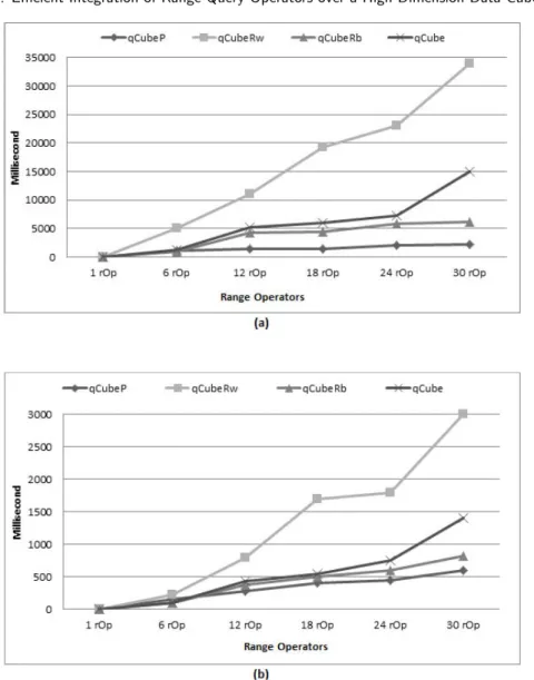
4.2 Performance Evaluation of Range Query Operators and Skewed Relations
Fig. 6. Response time queries with one infrequent point operator:T= 107
;C= 5000;D= 30;S= 2
.5.
two range operators (12op) and so on. We have at most five different range operators in a query with thirty operators (30op). Range operators are not implemented by Frag-Cubing.
Range operators areiOp =(greater than, different, less than, some, between). Figures 6 (a) and (b) illustrate scenarios where every range operator results have a frequent attribute, thus large TID sets intersections occur (qCubeRw).
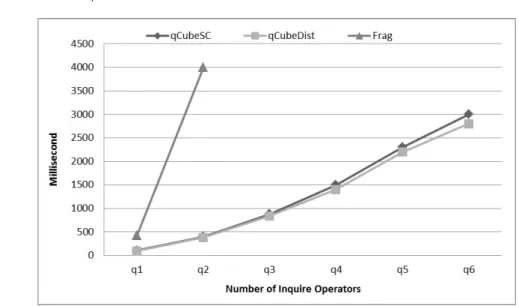
Fig. 7. Response time queries with inquire operators: T= 107
;C= 5000;D= 30;S= 2
.5.
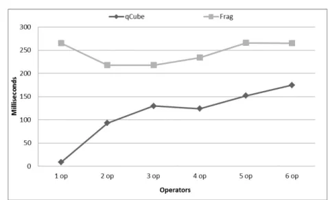
4.3 Performance Evaluation of Inquire Operators and Skewed Relations
Inquire operators are classified into sub-cube and distinct. Figure 7 illustrates tests using the same skewed relationR used in previous tests. We compareqCube sub-cube (qCubeSC) response times with Frag-Cubing implementation. The distinct operator (qCubeDist), as well as all range operators, are not implemented by Frag-Cubing. Frag-Cubing response times are by far slower than qCube. Queries with more than two sub-cube operators cannot be answered by Frag-Cubing, since there is not enough continuous memory in 128GB of RAM to allocate many big size arrays with many empty cells. Frag-Cubing duplicates an array size when it reaches its limit. In contrast,qCube has a linear response time as the number of inquire operators increases. The number of small complementary arrays makes it possible for qCube to produce huge amount of summarized results. Dimension rearrangements based on cardinalities also reduce inquire query response times drastically.
4.4 Cube Computation and Massive Experiments
Figure 8 illustratesqCubeand Frag-Cubing linear computation behavior as the number of dimensions increases. Tests use relations withS=0,107
T andC= 5000. Full, iceberg, dwarf, closed, MCG and many other cube approaches have exponential computation behavior as the number of dimensions increases. Frag-Cubing approach is faster to compute a data cube thanqCube. This is because both Frag andqCube are array based solutions, but Frag-Cubing allocates a new array twice as big as the previous one when a limit is reached. Therefore, there are few reallocations and a unique continuous array with lots of empty cells. Instead, qCube allocates complementary continuous arrays with small size, thus we have more reallocations, more arrays, but fewer empty cells. Fast Util framework encapsulates the set of complementary arrays in a Map data structure with constant access time.
Fig. 8. Runtime ofqCubeand Frag with different dimensions:T= 107
;C= 5000;S= 0.
Fig. 9. qCubememory consumption versus original relation disk space:T= 107
;C= 5000;S= 0.
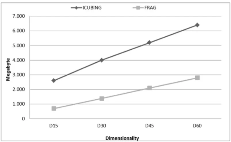
4.5 Memory Consumption
Figure 9 illustrates the linear memory consumption behavior ofqCube. Input is the original relation stored on disk. qCube is a data cube stored in RAM. AqCube with 60 dimensions and107of tuples
consumes 6.5GB of RAM versus 2.8GB of the original relation on disk. The massiveqCube with 60 dimensions and 100M tuples consumes 70GB of RAM and the original relation has 26GB on disk. In general,qCube uses 2.5x more memory to compute cubes from massive relations.
5. CONCLUSIONS AND FUTURE WORK
with slower insertion time. When compared with Frag-Cubing,qCube is faster to answer point and inquire queries with sub-cube operators. A cardinality sorting optimization demonstrates an enormous benefit, since a query often has at least one point sub-query with an infrequent attribute. Complex and costly inquire queries are efficiently answered byqCube. Frag-Cubing, in contrast, cannot answer two sub-cube operators in a data cube with 107 tuples,
C= 5000, D= 30and S= 2.5. The reason is that Frag-Cubing implements a single array with double size increase factor, so there is waste of memory.
There are many improvements to qCube. First, we must experiment it with holistic measures. Update and computation experiments with many holistic measures are a hard problem, but qCube
has an efficient design capable of addressing a solution to this problem with few adaptations. TIDs can become huge, thus memory consumption and intersection costs can become impracticable, and therefore we must address an efficient solution to partition TIDs with fast data retrieval. TheqCube
partition strategy using inverted tuples and measures is well designed for high performance computing architectures. Multicore and multicomputer versions ofqCube must be implemented. Top-k or rank queries are very useful for decision making, thereforeqCubemust be improved to answer top-k queries combined with range, point and inquire queries. Experiments with high dimensional text cubes must be made to evaluateqCube, specially its text measures computing.
REFERENCES
Brahmi, H.,Hamrouni, T.,Messaoud, R.,and Yahia, S. A New Concise and Exact Representation of Data
Cubes. In Advances in Knowledge Discovery and Management. Studies in Computational Intelligence, vol. 398. Springer Berlin Heidelberg, pp. 27–48, 2012.
Chan, C.-Y. and Ioannidis, Y. E. Bitmap Index Design and Evaluation. InProceedings of the ACM SIGMOD
International Conference on Management of Data Conference. Seattle, Washington, USA, pp. 355–366, 1998.
Chun, S.-J.,Chung, C.-W.,and Lee, S.-L.Space-Efficient Cubes for OLAP Range-Sum Queries.Decision Support
Systems37 (1): 83 – 102, 2004.
Gray, J.,Chaudhuri, S.,Bosworth, A.,Layman, A.,Reichart, D.,Venkatrao, M.,Pellow, F.,and
Pira-hesh, H.Data Cube: a relational aggregation operator generalizing group-by, cross-tab, and sub-totals.Data Mining
and Knowledge Discovery1 (1): 29–53, 1997.
Han, J.Data Mining: concepts and techniques. Morgan Kaufmann Publishers Inc., San Francisco, CA, USA, 2011.
Ho, C.-T.,Agrawal, R.,Megiddo, N.,and Srikant, R. Range Queries in OLAP Data Cubes. InProceedings
of the ACM SIGMOD International Conference on Management of Data Conference. Tucson, Arizona, USA, pp. 73–88, 1997.
Lee, S. Y.,Ling, T. W.,and Li, H.-G. Hierarchical Compact Cube for Range-max Queries. In Proceedings of
International Conference on Very Large Data Bases. San Francisco, CA, USA, pp. 232–241, 2000.
Leng, F.,Bao, Y.,Yu, G.,Wang, D.,and Liu, Y.An Efficient Indexing Technique for Computing High Dimensional
Data Cubes. InProceedings of the International Conference on Advances in Web-Age Information Management. Hong Kong, China, pp. 557–568, 2006.
Li, X.,Han, J.,and Gonzalez, H. High-Dimensional OLAP: a minimal cubing approach. InProceedings of the
International Conference on Very Large Data Bases. Toronto, Canada, pp. 528–539, 2004.
Liang, W.,Wang, H.,and Orlowska, M. E. Range Queries in Dynamic OLAP Data Cubes. Data & Knowledge
Engineeering34 (1): 21 – 38, 2000.
Lima, J. d. C. and Hirata, C. M. Multidimensional Cyclic Graph Approach: representing a data cube without
common sub-graphs. Information Sciences181 (13): 2626–2655, 2011.
Ruggieri, S.,Pedreschi, D.,and Turini, F. Dcube: discrimination discovery in databases. InProceedings of ACM
SIGMOD International Conference on Management of data. New York, NY, USA, pp. 1127–1130, 2010.
Sismanis, Y.,Deligiannakis, A.,Roussopoulos, N.,and Kotidis, Y.Dwarf: shrinking the petacube. InProceedings
of the ACM SIGMOD International Conference on Management of Data Conference. New York, NY, USA, pp. 464– 475, 2002.
Xin, D., Shao, Z., Han, J.,and Liu, H. C-cubing: efficient computation of closed cubes by aggregation-based