REPOSITORIO INSTITUCIONAL DA UFOP: Dynamic topic herarchies and segmented rankings in textual OLAP technology.

Dynamic Topic Hierarchies and

Segmented Rankings in Textual OLAP

Technology

Aluno: Adriano Neves de Paula e Souza

Orientador: Joubert de Castro Lima

Universidade Federal de Ouro Preto

ii

Disserta¸c˜ao de autoria de Adriano Neves de Paula e Souza, sob o t´ıtulo “Dynamic Topic

Hierarchies and Segmented Rankings in Textual OLAP Technology”, apresentada

ao Departamento de Computa¸c˜ao da Universidade Federal de Ouro Preto, para obten¸c˜ao do t´ıtulo de Mestre em Ciˆencia da Computa¸c˜ao pelo Programa de P´os-gradua¸c˜ao em

Ciˆencia da Computa¸c˜ao, aprovada em 20 de Julho de 2017 pela comiss˜ao julgadora constitu´ıda pelos doutores:

Prof. Dr. Ricardo Rodrigues Ciferri

Universidade Federal de S˜ao Carlos (UFSCAR)

Prof. Dr. Rodrigo Rocha Silva

Faculdade de Tecnologia de Mogi das Cruzes (FATEC-MC) / Centro de Inform´atica e Sistemas da Universidade de Coimbra (CISUC)

Prof. Dr. Reinaldo Silva Fortes

Catalogação: www.sisbin.ufop.br

S895d Souza, Adriano Neves de Paula e .

Dynamic topic hierarchies and segmented rankings in textual OLAP technology [manuscrito] / Adriano Neves de Paula e Souza. - 2017. 82f.: il.: color; grafs; tabs.

Orientador: Prof. Dr. Joubert de Castro Lima.

Dissertação (Mestrado) - Universidade Federal de Ouro Preto. Instituto de Ciências Exatas e Biológicas. Departamento de Computação. Programa de Pós-Graduação em Ciência da Computação.

Área de Concentração: Ciência da Computação.

1. Administração de dados. 2. Dados textuais. 3. Classificação. 4. Cubo de dados. I. Lima, Joubert de Castro . II. Universidade Federal de Ouro Preto. III. Titulo.

Dedico este trabalho `a minha fam´ılia.

Dynamic Topic Hierarchies and Segmented Rankings in

Textual OLAP Technology

Resumo

A tecnologia OLAP tem se consolidado h´a 20 anos e recentemente foi redesenhada para que suas dimens˜oes, hierarquias e medidas possam suportar as particularidades dos dados textuais. A tarefa de organizar dados textuais de forma hier´arquica pode ser resolvida com a constru¸c˜ao de hierarquias de t´opicos. Atualmente, a hierarquia de t´opicos ´e definida apenas uma vez no cubo de dados, ou seja, para todo o lattice de cuboides. No entanto, tal hierarquia ´e sens´ıvel ao conte´udo da cole¸c˜ao de documentos, portanto em um mesmo cubo de dados podem existir c´elulas com conte´udos comple-tamente diferentes, agregando cole¸c˜oes de documentos distintas, provocando potenciais altera¸c˜oes na hierarquia de t´opicos. Al´em disso, o segmento de texto utilizado na an´alise OLAP tamb´em influencia diretamente nos t´opicos elencados por tal hierarquia. Neste trabalho, apresentamos um cubo de dados textual com m´ultiplas e dinˆamicas hierar-quias de t´opicos. M´ultiplas por serem constru´ıdas a partir de diferentes segmentos de texto e dinˆamicas por serem constru´ıdas para cada c´elula do cubo. Outra contribui¸c˜ao deste trabalho refere-se `a resposta das consultas multidimensionais. O estado da arte normalmente retorna os top-k documentos mais relevantes para um determinado t´opico. Vamos al´em disso, retornando outros segmentos de texto, como os t´ıtulos mais signifi-cativos, resumos e par´agrafos. A abordagem ´e projetada em quatro etapas adicionais, onde cada passo atenua um pouco mais o impacto da constru¸c˜ao de v´arias hierarquias de t´opicos e rankings de segmentos por c´elula de cubo. Experimentos que utilizam parte dos documentos da DBLP como uma cole¸c˜ao de documentos refor¸cam nossas hip´oteses.

Dynamic Topic Hierarchies and Segmented Rankings in

Textual OLAP Technology

Abstract

The OLAP technology emerged 20 years ago and recently has been redesigned so that its dimensions, hierarchies and measures can support the particularities of textual data. Organizing textual data hierarchically can be solved with topic hierarchies. Currently, the topic hierarchy is defined only once in the data cube, e.g., for the entire lattice of cuboids. However, such hierarchy is sensitive to the document collection content. Thus, a data cube cell can contain a collection of documents distinct from others in the same cube, causing potential changes in the topic hierarchy. Furthermore, the text segment used in OLAP analysis also changes this hierarchy. In this work, we present a textual data cube with multiple dynamic topic hierarchies for each cube cell. Multiple hierar-chies, since the presented approach builds a topic hierarchy per text segment. Another contribution of this work refers to query response. The state-of-the-art normally returns the top-k documents to the topic selected in the query. We go beyond by returning other text segments, such as the most significant titles, abstracts and paragraphs. The approach is designed in four complementary steps and each step attenuates a bit more the impact of building multiple topic hierarchies and segmented rankings per cube cell. Experiments using part of the DBLP papers as a document collection reinforce our hypotheses.

Declara¸c˜

ao

Esta disserta¸c˜ao ´e resultado de meu pr´oprio trabalho, exceto onde referˆencia expl´ıcita ´e feita ao trabalho de outros, e n˜ao foi submetida para outra qualifica¸c˜ao nesta nem em outra universidade.

Adriano Neves de Paula e Souza

Agradecimentos

Agrade¸co primeiramente `a minha fam´ılia por ter me apoiado em mais uma etapa de minha vida, me dando suporte nos momentos cr´ıticos em que eu mais precisava. Agrade¸co ao meu pai Jos´e Silv´erio de Souza por sempre estar disposto a sair de Ipatinga e ir a Ouro Preto me dar o suporte necess´ario, seja em casos de sa´ude ou apenas saudade. Agrade¸co `a minha m˜ae Maria Petronilha de Paula e Souza por ser a chave principal da minha vida. A pessoa que sempre me incentivou a seguir o caminho do estudo e que sempre acreditou no meu potencial, at´e mesmo em momentos em que nem eu acreditava. Dedico todas as conquistas da minha vida `a minha m˜ae, que sempre investiu em minha sabedoria sem nunca exigir nada em troca, esperando apenas o meu sucesso. Agrade¸co tamb´em `as minhas irm˜as Silv´eria Neves de Paula e Souza e Juliana Neves de Paual e Souza, pela cumplicidade e amor incondicional, sempre servindo como parˆametro de car´ater e sabedoria.

Agrade¸co tamb´em ao meus orientadores Joubert de Castro Lima e Reinaldo Silva Fortes pela paciˆencia e compreens˜ao neste trabalho. Dois professores excelentes com ideias geniais que possibilitaram um trabalho digno onde nos orgulhamos. Agrade¸co ao Joubert pelas ideias geniais e pelo prazer de trabalhar com OLAP. Mesmo em momentos conturbados, esteve sempre disposto a me orientar da melhor forma poss´ıvel, me apoi-ando e me dapoi-ando suporte necess´ario, independente da hora ou do dia. Agradecimento especial tamb´em ao Reinaldo, pe¸ca essencial nesta equipe, com ideias geniais e conheci-mento valioso, sempre somando ao nosso trabalho. Muito obrigado pela disposi¸c˜ao em atender `as minhas chamadas independente da hora ou do dia, sempre arrumando um tempinho para discutirmos d´uvidas e ideias novas.

Agrade¸co ao meu amigo Tales Mota por estar sempre disposto a me ajudar com qualquer d´uvida, seja em um artigo complicado, ou com um c´odigo problem´atico, sua boa vontade sempre fez a diferen¸ca.

Agrade¸co tamb´em `a minha namorada Fernanda Camini pelo carinho e compreens˜ao nos momentos mais dif´ıceis dessa jornada.

Agrade¸co `a CAPES pelo aux´ılio financeiro a este projeto e agrade¸co `a UFOP pela infraestrutura cedida e conhecimento oferecido.

Muito Obrigado.

Sum´

ario

Lista de Figuras xv

Lista de Tabelas xvii

1 Introduction 1

2 Basic Concepts 5

2.1 Data Warehouse . . . 5

2.2 Data Cube . . . 7

2.2.1 Cube Cell . . . 9

2.2.2 Measures . . . 10

2.2.3 Concept Hierarchies . . . 11

2.2.4 Topic Hierarchy . . . 13

2.3 OLAP . . . 14

2.3.1 OLAP Operations . . . 15

2.4 CATHY (Contructing A Topical Hierarchy) . . . 17

2.4.1 Definitions . . . 18

2.5 Information Retrieval . . . 20

3 Related Works 23

4 DTCubing Approach 27

4.1 Text Segments . . . 27

4.2 Data Cube and Cube Cell Concepts . . . 28

4.3 Multiple Topic Hierarchies per Cube Cell . . . 29

5 DTCubing Architecture 31 5.1 Indexing . . . 32

5.2 Filtering . . . 35

5.3 Hierarchy Generation . . . 37

5.4 Ranking . . . 39

6 Hypothesis Validation 41 6.1 Multiple Topic Hierarchies Qualitative and Quantitative Analysis . . . . 42

6.2 Segmented Rankings Quantitative Analysis . . . 46

7 Performance Evaluation 49 7.1 Indexing Step Runtime . . . 49

7.2 Filtering Step Runtime . . . 50

7.3 Hierarchy Generation Runtime . . . 52

7.4 Ranking Runtime . . . 53

8 Conclusion 55

Referˆencias Bibliogr´aficas 57

Lista de Figuras

2.1 OLAP operation example. . . 6

2.2 Geometric 3D data cube. . . 8

2.3 Geometric 4D data cube. . . 9

2.4 4D data cube lattice. . . 10

2.5 Location and Time concept hierarchies . . . 12

2.6 Hierarchies build from Location and Time structured dimensions . . . 13

2.7 Literature topic hierarchy. . . 14

2.8 OLAP operation example. . . 16

4.1 DTCubing approach . . . 29

5.1 DTCubing Architecture steps . . . 32

5.2 Hierarchy Generation example . . . 37

5.3 Ranking example . . . 39

6.1 Hierarchies from DTCubing cells versus hierarchies from GH cells . . . . 42

6.2 Hierarchies built from the text segments title, abstract, and sentence from VLDB conference . . . 43

6.3 Heat maps comparing GH and DTCubing hierarchies . . . 45

6.4 Entropy values of GH and different DTCubing hierarchies . . . 46

6.5 Jaccard ranking values from GH versus DTCubing for ACM conference . 48

7.1 Runtimes of the hierarchy generation algorithm . . . 52

7.2 Runtimes of the segment rankings construction algorithm . . . 53

Lista de Tabelas

2.1 2-D data cube. . . 7

2.2 3D data cube. . . 8

2.3 Inverted Index example. . . 21

3.1 Comparison of literature approaches with DTCubing . . . 26

5.1 Indexing Step example. . . 33

5.2 Attribute values . . . 36

5.3 Aggregation Values . . . 36

7.1 Runtime for the Indexing step for document collectionDOC₁,DOC₂ and DOC₃ . . . 50

7.2 Point, range and inquire filters . . . 50

7.3 Runtimes (seconds) of point, range and inquire filters . . . 51

Lista de Algoritmos

5.1 Indexing Step Algorithm . . . 34

5.2 Filtering Step Algorithm . . . 37

5.3 Hierarchy Generation Step Algorithm . . . 38

5.4 Ranking Step Algorithm . . . 40

“Quando o poder do amor superar o amor pelo poder, o mundo conhecer´a a paz.”

— Jimi Hendrix

Chapter 1

Introduction

The popularization of social networks (e.g., Facebook, Twitter and Instagram) and mul-timedia aggregators (e.g., YouTube and Wikipedia) increased in great amount the vol-ume of textual data (Cuzzocrea, De Maio, Fenza, Loia & Parente 2016). This scenario turns the work of managers, executives and data analysts very hard , since the volume of documents has far exceeded the human capacity for understanding texts (Tseng & Chou 2006). This analysis bottleneck is the starting point to our demand for remodeling traditional Online Analytical Processing (OLAP) tools, once they become inadequate for textual data type (Bouakkaz, Loudcher & Ouinten 2016).

The data cube operator (Gray, Chaudhuri, Bosworth, Layman, Reichart, Venkatrao, Pellow & Pirahesh 1997), being the core of any OLAP tool, faces new challenges and impossibilities when applied to multidimensional textual databases. Its hierarchies, usu-ally modeled by a specialist and only once during the cube lifecycle, are not useful, since they do not consider the semantic relations among documents and the dynamics of the hierarchical levels of the document collection.

Hierarchies are fundamental in the decision-making process because they allow the mapping of low level concepts into high level concepts (Gray, Chaudhuri, Bosworth, Layman, Reichart, Venkatrao, Pellow & Pirahesh 1997). Thus, they reduce the search space and, usually, streamline and simplify user analysis. It is intuitive to understand that the year attribute is hierarchically higher than day, but when the attribute is a collection of documents, how can we detect if a term, a text segment or even the entire document is hierarchically higher or lower than another one? Different textual cube approaches emerge to solve the challenge of navigating through structured and textual

2 Introduction

data in an integrated manner (Lin, Ding, Han, Zhu & Zhao 2008, EventCube: Multi-Dimensional Search and Mining of Structured and Text Data2013, Yu, Lin, Sun, Chen, Han, Liao, Wu, Zhai, Zhang & Zhao 2009, Zhang, Zhai & Han 2009, Zhang, Zhai & Han 2011).

Topic hierarchy is a useful alternative to organize a document collection in a hierar-chy (Zhang, Zhai & Han 2009). A topic consists of specific concepts of a subject area (Gallinucci, Golfarelli & Rizzi 2013). For instance, let’s consider the topic “economy”, representing several entries of a document collection, like “the dollar in the world be-comes high in 2016”’, “smartphone sales reach 85% of Brazilian consumers”, “Will USA change their economy politics?” and many others. The “economy” topic represents all previous entries, and sometimes a topic is not present in the document collection. There is a clear advantage in topic concept because it reduces data volume and represents better the entire document collection. Topic hierarchies are built automatically with methods like CATHY (Wang, Danilevsky, Desai, Zhang, Nguyen, Taula & Han 2013) orHpam (Mimno, Li & McCallum 2007), or manually by domain specialists.

Unfortunately, the literature in textual OLAP, that supports the concept of topic hierarchy, still suffers from serious limitations since they assume the creation of this hierarchy only once and for the entire document collection. This way, a topic t₁ is always hierarchically higher than topic t₂, regardless the selected cube cell in a query. The first hypothesis of this work assumed that it is not enough to build a single topic hierarchy from the entire document collection in order to meet the specific needs of the users, but rather to build dynamic topic hierarchies from subsets of all documents. When making a query, the user often defines filters that select cube cells with subsets of documents of interest. Then, these filters should guide the construction of a new topic hierarchy, presenting more exclusive and specific topics to the subset selected, improving the decision-making process.

The textual OLAP query’s results also undergo through advances in order to better represent the particularities of textual data. The literature computes measures to rank relevant documents using different strategies (Lin, Ding, Han, Zhu & Zhao 2008, Zhang, Zhai & Han 2009, Zhang, Zhai & Han 2011, Oukid, Asfari, Bentayeb, Benblidia & Boussaid 2013, Janet & Reddy 2011, Liu, Tang, Hancock, Han, Song, Xu, Manikonda & Pokorny 2012, Lee, Kim & Kim 2014). Our second hypothesis is that many queries aim to return rankings of more specific text segments, such as paragraph, abstract, chapter,

Introduction 3

relevant book chapters or even a list of the more relevant documents about this topic. In this work we present a new textual OLAP approach named Dynamic Topic Cubing, or DTCubing for short, that builds topic hierarchies per textual cube cell instead of a single hierarchy per cube lattice and it also supports multiple hierarchies per cube cell, since a document can be partitioned into several text segments (e.g.,title,keywords, and

abstract). DTCubing can create multiple top-k rankings according to the defined text segments.

Experimental evaluations reinforced our hypothesis. Some conferences that compose the DBLP1 were used to conduct our performance evaluation. A new algorithm, based on the qCube approach (Silva, Lima & Hirata 2013), was implemented to compute both multiple topic hierarchies and multiple segmented rankings.

The main contributions of this work are:

i) a new data cube model for textual OLAP, where each cube cell has several topic hierarchies and several rankings, both according to different text segments;

ii) a new textual OLAP partial cube algorithm that attenuates the impact of building multiple topic hierarchies and segmented rankings per cube cell;

iii) qualitative and quantitative evidences to reinforce the hypothesis;

iv) a performance study to validate the algorithm runtimes in the presence of various collections of documents and queries.

The remainder of this work is organized as follows: Chapter 2 presents the basic concepts of this work, in Chapter 3, the related work used to produce DTCubing is presented. Chapter 4 presents the formal definition of a DTCubing cube. In Chapter 5, the four steps that compose the DTCubing approach are explained. Chapter 6 presents the experiments conducted for the consolidation of the hypotheses, proving the usefulness of the DTCubing approach. In Chapter 7 , a performance evaluation, presents the four DTCubing algorithm steps runtimes. In the Conclusion Chapter, we present the final discussions and how DTCubing can be improved in future works.

Chapter 2

Basic Concepts

In this chapter, the basic concepts related to this dissertation are presented. Section 2.1 presents the main concepts of Data Warehouse. Section 2.2 presents the main con-cepts of data cubes, presenting its measures, cells and describing the difference between the hierarchies built for structured and textual dimensions. Section 2.3 brings a brief description of the OLAP concept, presenting its main operations. Section 2.4 presents the automatic model for building topic hierarchies named CAHY. Finally, section 2.5 presents a summary of the main stages of the process of Information Retrieval (IR).

2.1

Data Warehouse

A Data Warehouse is a subject-oriented, integrated, time-variant, and nonvolatile collec-tion of data in support of management’s decision making process (Inmon & Hackathorn 1994). The four keywords, subject-oriented, integrated, time-variant, and nonvolatile, differentiate DW from other repository systems, such as relational database systems, transaction processing systems, and file systems.

A DW models, in an integrate manner, important subjects, such as customer, sup-plier, product and sales, for decision makers and not for the day-to-day operations. Hence, DWs typically exclude data that are not useful in the decision support process.

Normally, a DW integrates heterogeneous data sources, such as relational tables, flat-files, serialized objects, and XML files, into a unique analytical data source. Data cleaning and data integration techniques are applied to ensure consistency in naming

6 Basic Concepts

conventions, dimension structures, attribute measure, and so on.

Typically, the DW is maintained separately from the organization’s operational databases. There are many reasons for doing this. The DW supports on-line ana-lytical processing (OLAP), the functional and performance requirements of which are quite different from those of the on-line transaction processing (OLTP) applications tranditionally supported by the operational databases (Chaudhuri & Dayal 1997).

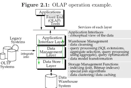
In (Wu & Buchmann 1997), the authors propose a logical architecture for a DW. Fig-ure 2.1 illustrate such an architectFig-ure. Each layer provides services for the next higher layer, or for the intralayer process. The Data Store Layer provides the Data Manage-ment Layer the services for storing the data, building indexes (Bitmap indexes, or special join indexes), data clustering, etc. The Data Management Layer, in turn, provides ser-vices for higher level management of warehouse data, e.g., load utilities, data model transformation between external sources and the logical schema, data cleansing, query processing, query optimization, etc. Next, the Application Interface Layer provides data access facilities suitable for specific applications, including data model transformation between the conceptual multidimensional schema and the logical schema. The Presen-tation Layer includes graphical presenPresen-tation and reporting tools. It typically runs on a desktop environment whereas the other three layers typically exist on the server side. The presentation layer therefore also includes the desktop resident processes needed for extract generation (Wu & Buchmann 1997).

Basic Concepts 7

2.2

Data Cube

DWs and OLAP tools are based on a multidimensional model. The multidimensional model views the stored data as a data cube. A data cube allows to be modeled and viewed in multiple dimensions. It is defined by dimensions and facts. (Han, Kamber & Pei 2011)

In general terms, dimensions are perspectives of the decision making process. They are modeled as an entity or a set of entities that encapsulate a concept. For example UFOP may create a grade DW in order to keep records of the institute grades with respect to the dimensions time, student, professor, department, and discipline. The dimensions allow grade analysis from different perspectives. We can obtain the grades of each semester of the last ten years in the university or the grades of a specific student in 2008 or the grades of a specific department or discipline.

Each dimension has a set of attributes that describes it. For example, the dimension

studentmay contain the attributesfirst-name,last-name, sex, andbirth-date. As men-tioned before, each dimension is modeled as a single entity or a set of entities, so the set of attributes must be organized in such entity(ies).

A multidimensional data model is typically organized around a central theme, such as grade. The theme is represented by facts. A fact is the minimum amount of information to be analyzed, i.e., the quantity by which we want to analyze relationship among dimensions.

Table 2.1: 2-D data cube.

Discipline

Time Math1 Math2 Physic1 Logic

Q1 78.5 77.8 72.5 87.5

Q2 79 77.5 71.8 78.9

Q3 71.2 78 73 81.6

Q4 78.5 74.8 71.5 86.5

8 Basic Concepts

dimensions time and discipline. The data cube is shown in Table 2.1. In the 2-D representation, the grades are shown with respect to the time dimension (organized in quarters) and the discipline dimension (organizes according to the disciplines offered at UFOP). The fact or measure displayed is grade (the average grade, for instance).

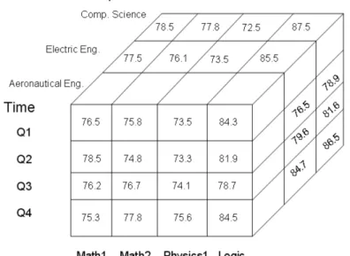
Now, we extend the initial idea, adding a third dimension to UFOP grade data cube. We add the dimension department, forming a new data cube with dimensions time,

discipline, anddepartment. The 3-D data cube, presented in Table 2.2, is represented as a series of 2-D tables. Conceptually, we may also represent the same data as a 3-D data cube, presented in Figure 2.2.

Table 2.2: 3D data cube.

Department

Aeronautical Eng. Eletric Eng. Computer Science

Discipline Discipline Discipline

Time Math1 Math2 Physic Logic Math1 Math2 Physic Logic Math1 Math2 Physic Logic

Q1 76.5 75.8 73.5 71.2 69.4 74.6 77.1 71 73.1 72.5 74.1 77.9

Q2 72.4 77.7 78.3 82.4 69.3 72.5 77.3 71.9 71.2 71.3 77.5 82.4

Q3 77.2 78 79.3 72 77.1 73.2 74.8 79.6 69.4 72.6 80 80.4

Q4 75.3 77.8 84.5 77.3 72.5 94.7 78.5 75.8 75.6 74.8 71.5 88.5

Basic Concepts 9

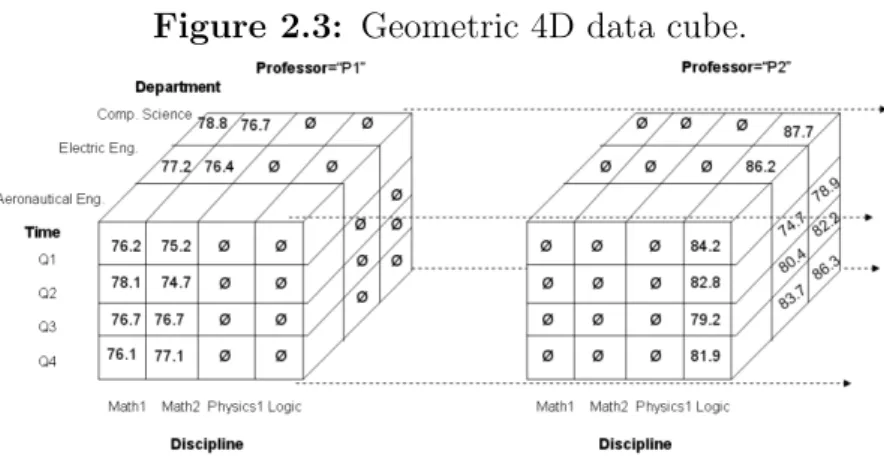
Extending the 3-D UFOP data cube, we can add a fourth dimension such as pro-fessor. It is possible to think of a 4-D data cube as being a series of 3-D data cubes, as shown in Figure 2.3.

Figure 2.3: Geometric 4D data cube.

It is possible to continue in this way, so it is possible to display an-D data cube as a series of (n−1)-D data cubes. In Figure 2.3, the symbol Øis an empty cell, indicating that a professor does not teach the discipline.

The described tables (2-D and 3-D) show the data at different degrees of summa-rization. Each summarized table is a cuboid. Given a set of dimensions, it is possible to generate a cuboid for each of the possible subsets of the given dimensions. The result forms a lattice of cuboids, each sowing the data at different level of summarization, or group-by. The lattice ofcuboids is the referred to as a data cube. In Figure 2.4, is rep-resented a 4-D cube as a lattice ofcuboids formed from the dimensiontime, professor,

department, and discipline.

Thecuboid that holds the lowest level of summarization is called the basecuboid. For example, the 4-Dcuboid in Figure 2.4 is the basecuboid for the given dimensionstime,

professor, department, and discipline. The 0-D cuboid which holds the highest summarization, is called the apex cuboid. In the UFOP grade DW, this is the average grade, summarized over all four dimensions. The apex cuboid is typically denoted by all.

2.2.1

Cube Cell

10 Basic Concepts

more dimensions, where each dimension is indicated by a wildcard all(“*”) in the cell notation.

Figure 2.4: 4D data cube lattice.

Suppose there is ann-dimensional data cube. Let a= (a₁, a₂, a₃, a_n, measures) be a cell from on of thecuboids making up the data cube. Cell a is anm-dimensional cell (that is, from an m-dimensional cuboid) if exactly (m(m = n)) values among {a₁, a₂, a₃, an}

are not “*”. Ifm =n, then ais a base cell; otherwise, it is an aggregate cell (i.e., where

m < n).

Consider a data cube with dimensions, time, department and discipline, and the measure grade . Cells (Q1,∗,∗,78.9) and (∗,comp. science,∗,81.3) are 1-D cells, (Q1, M ath1,73.6) is a 2-D cell and (Q1,comp. science,M ath1,78.8) is a 3-D cell. Here, all base cells are 3-D, whereas 1-D and 2-D cells are aggregate cells.

2.2.2

Measures

A data cube is composed by several cuboids and each cuboid is composed by several cube cells. Each cube cell can be defined as a pair < {d₁, d₂, d_n}, measures > , where

{d₁, d₂, dn}represents a possible combination of attribute values over the dimensions. A

data cube measure is a numerical function that can be evaluated at each cell in the lattice. A measure value is computed for a given cell by aggregating the data corresponding to the attribute values defining the given cell.

Measures can be organized into three categories, based on the kind of aggregate functions used. The categories are: distributive, algebraic and holistic.

Basic Concepts 11

resulting in n aggregate values. If the result derived by applying the function to the n

aggregate values is the same as that derived by applying the function to the entire data set (without partitioning), the function can be computed in a distributive manner. For example, count() can be computed for each subcube, and then summing up the counts obtained for each subcube. Hence, count() is a distributive aggregate function. For the same reason,sum(),min(), and max()are distributive aggregate functions. Distributive measures can be computed efficiently because they can be computed in a distributive manner.

An aggregate function is algebraic if it can be computed by an algebraic function with

M arguments (whereM is a bounded positive integer), each of argument is obtained by applying a distributive aggregate function. For example,avg()(average) can be computed by sum()/count(), where both sum() and count() are distributive aggregate functions. Similarly, it can be shown that min-N() and max-N() (which find theN minimum and

N maximum value, respectively, in a given set) and standard-deviation() are algebraic aggregate functions. A measure is algebraic if it is obtained by applying an algebraic function.

An aggregate function is holistic if there is no constant bound on the storage size needed to describe a sub-aggregate, i.e., there is not an algebraic function withM argu-ments (where M is a constant) that characterizes the computation. Common examples of holistic function include median(), mode(), and rank(). A measure is holistic if it is obtained by applying a holistic aggregate function.

Most of the current data cube technology confines the measure of multidimensional databases to numerical data. However, measures can also be applied to other kinds of data, such as spatial, multimedia, or text data.

2.2.3

Concept Hierarchies

12 Basic Concepts

Many concept hierarchies are implicit within the database schema. For example, suppose that UFOP is composed by several divisions, located at different regions of Brazil. A new dimension nameddivision locationmay be required. The new dimension can be described by the attributes: country, state and city. the attributes are related by a total order, forming a concept hierarchy such as “country state city”. The hierarchy is show in Figure 2.5(a). Alternatively, the attributes of a dimension may be organized as a partial order, forming a lattice. An example of a partial order for the

time dimension based on the attributes: year, month, week, and day is“year month week day”. This lattice structure is shown in Figure 2.5(b).

(a) Location di-mension concept hierarchy.

(b) Time dimension concept hi-erarchy.

Figure 2.5: Location and Time concept hierarchies

A concept hierarchy that is total or partial order among attributes in a database schema is called a schema hierarchy. There may be more than one concept hierarchy for a given attribute or dimension, based on different user perspectives. Concept hierarchies may be provided manually by system users, domain experts, or knowledge engineers, or may be automatically generated based on statistical analysis of the data distribution.

It is important to note that although there are automatic building strategies for hierarchies of the structured dimensions, this kind of hierarchy is usually built manually, being provided by a specialist. Furthermore, these hierarchies are built only once and kept throughout the life cycle of the cube.

Basic Concepts 13

the attributeState, just as it is intuitive to know that Yearis hierarchically higher to

Day. However, when we are working with a textual dimension, the hierarchization task becomes a little more complex. The problem is to know if a documentd_i is hierarchically higher or lower to a documentd_j. In order to do that, the most commonly used strategy in the literature is the utilization of a Topic Hierarchy.

2.2.4

Topic Hierarchy

A Topic Hierarchy is a structure presented as a tree, which allows the semantic mapping of a set of documents in different nodes, allowing OLAP operations such as drill-down and roll-up in the textual dimension. Thus, a topic hierarchy hierarchizes documents through their contents, presenting in each node, a set of topics in which the user is more likely to be interested.

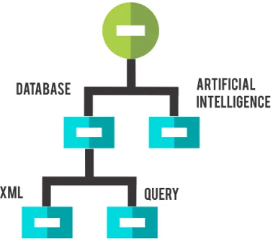
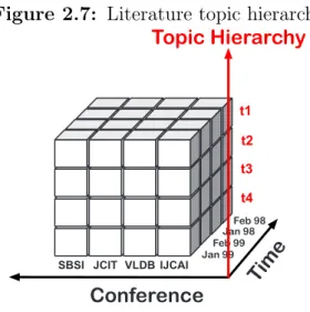
Figure 2.6 shows a topic hierarchy built on a set of scientific articles that belong to DBLP. Observe the dynamics offered for the data analysis. The user can navigate through the nodes of the topic hierarchy analyzing only the scientific articles which are about data base or only those which are aboutartificial intelligence.

Figure 2.6: Hierarchies build from Location and Time structured dimensions

14 Basic Concepts

that, regardless of the cell in which the user is, the documents aggregated there can only be analyzed under the perspective of the same four topics t1, t2, t3 and t4.

Since this topic hierarchy has to cover all the cells of the cube, it ends up presenting very generic topics, as it should present topics that represent all the collections of doc-uments. This can be understood as a deficiency of textual OLAP, once the user should be able to choose topics that were relevant only to the context of his/her query instead of being always limited to the same generic topics.

Figure 2.7: Literature topic hierarchy.

Conference T

ime

Jan 99 Feb 99

Jan 98Feb 98 Topic Hierarchy

t4 t3 t2 t1

SBSI JCIT VLDB IJCAI

Although it is static, the topic hierarchy can be built both manually and automat-ically. Manual building is used by most approaches, where the hierarchy is built and offered by a specialist, requiring time and being subject to errors. As for the automatic building of a topic hierarchy, it can be consolidated by using approaches such as CATHY (Wang, Danilevsky, Desai, Zhang, Nguyen, Taula & Han 2013) or HPAM (Mimno, Li & McCallum 2007), which use the analysis of a network of terms co-occurrence to find the main topics present in one base.

2.3

OLAP

Basic Concepts 15

OLAP tools present multidimensional data from DWs, regardless of how or where the data are stored. Each OLAP tool must handle a new abstract data type, named data cube, so it must consider data storage issues. OLAP tools use one of the following storage strategies: Relational OLAP (ROLAP), Multidimensional OLAP (MOLAP), Hybrid OLAP (HOLAP).

ROLAP tools use a relational or extended-relational Database Management System (DBSM) to store and management data cubes. They include optimizations for each DBMS back-end, implementation of aggregation navigation logic, and additional tools and services.

MOLAP tools implement multidimensional data structures to store data cubes effi-ciently, since they allow fast indexing to cube cells. With multidimensional data stores, the storage utilization may be low if the dataset is sparse. In such cases, reduction techniques should be explored.

HOLAP tools combine ROLAP and MOLAP. Normally, the detailed data are stored in relational database (ROLAP) and the aggregations are stored in multidimensional data structures (MOLAP).

2.3.1

OLAP Operations

In the multidimensional model, data are organized into multiple dimensions, and each dimension contains multiple levels of abstractions defined by concept hierarchies. This organization provides users/systems with the flexibility to view data from different per-spectives. A number of OLAP data cube operations exist to materialize these different views, allowing interactive querying and analysis of the data at hand (Han, Kamber & Pei 2011).

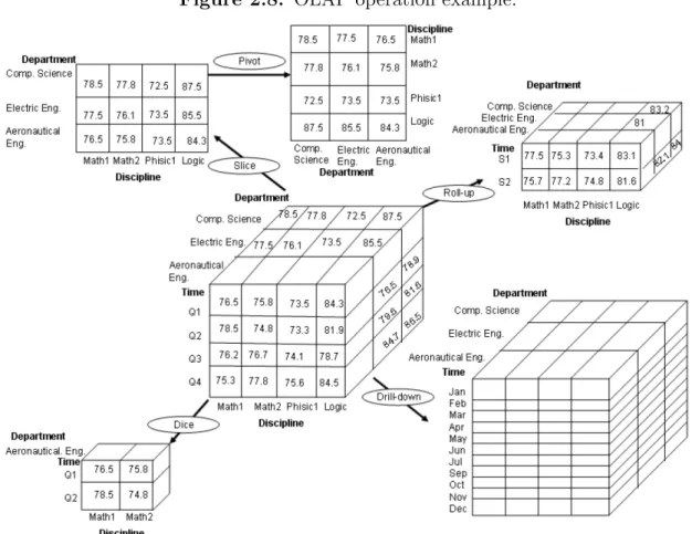
Figure 2.8 illustrates some typical OLAP operations for multidimensional data. At the center of the figure is a data cube for UFOP grade DW. The cube contains the di-mensionstime,department, anddiscipline, wheretimeis aggregated with respect to quarters,department is aggregated with respect to department names anddiscipline

16 Basic Concepts

Figure 2.8: OLAP operation example.

on the central cube by climbing up the concept hierarchy for time. This hierarchy is defined by a partial order “yearsemesterquartermonthday”, “yearweek

day”. The roll-up operation shows data aggregations by ascending the time hierarchy from the level of quarter (Q₁, Q₂, Q₃ and Q₄) to semester (S₁andS₂).

When roll-up is performed by dimension reduction, one or more dimensions are logi-cally removed from the given cube. For example, consider a grade data cube containing only the two dimensions department and discipline. Roll-up may be performed by removing time dimension, resulting in an aggregation of the grade by a department

and discipline, rather than by department, discipline and time.

Basic Concepts 17

to the more detailed level of month. The resulting data cube details thegrade per month rather than summarizing them by quarter.

Because drill-down adds more details to the given data, it can also be performed by adding new dimensions to a cube. For example, a drill-down on the central cube of Figure 2.8 can occur by introducing an additional dimension, such as professor or

student.

The slice operation performs a selection on one dimension of the given cube, resulting in a subcube. Figure 2.8 shows a slice operation where the grade data are selected from the central cube using the criteriontime= “Q′′₁. The dice operation defines a subcube by performing a selection on two or more dimensions. Figure 2.8 shows a dice operations on the central cube based on the following selection criteria that include three dimensions: (department= “AeronauticalEng.′′) and (discipline= “M ath1′′or“M ath2′′).

The pivot (rotate) operation rotates the data axes in order to provide an alternative presentation of the data. Figure 2.8 shows a pivot operation where the department

and discipline axes in a 2-D slice are rotated.

There are other OLAP operations. For example, drill-cross executes queries involving two or more fact tables of a fact constellation schema. The drill-through operation uses relational SQL facilities to drill through bottom level of a data cube down to its lower level. Other OLAP operations may include ranking the top K or bottom K items in lists, as well as computing growth rates, interests, internal rates of return, depreciation, and statistical functions.

Traditionally used for an analysis of structured data, OLAP has been developing each year to meet the needs for the analyses of non-structured data, such as geographical and textual data. This work focuses on textual OLAP, which has as main characteristic, the analysis and navigation of structured data together with textual data to assist Informa-tion Retrieval systems.

2.4

CATHY (Contructing A Topical Hierarchy)

18 Basic Concepts

CATHY works with databases of small texts, in particular, content-representative

documents. Acontent-representative document serves as a concise representation of the content of the complete document. For instance, the title of a scientific article is usually

content-representative document, as it is a good representation of the topics found in the complete article.

Besides serving as a concise representation of a document, content-representative

documents are used for the building of the topic hierarchy in CATHY because they are small, since the approach is extremely sensitive to the amount of terms. The larger the number of terms, the longer the time required to build the topic hierarchy.

Topic hierarchies built by CATHY are represented by an ordered list of “topical phrases”, where each child topic is a subset of the father topic. For example, the topics

query processing and optimization can be described by the phrases {“query process-ing”, “query optimization”,. . .}, whereas the father topic can be described by {“query processing”, “database systems”, “concurrency control”,. . .}.

CATHY is a “phrase-centric” framework to generate topic hierarchies via recursive clustering and ranking. Its main characteristics are:

• Phrase-centric approach: instead of using measures centered in unigrams, CATHY provides topics represented by phrases, that is, n-grams, as a result of its execution. The framework is able to mine and rank high quality phrases for each topic.

• Phrases ranking: a function of phrases ranking is defined, which implements four criteria that intuitively represent high quality phrases: coverage,purity,phraseness

and completeness. Through this it is possible to compare phrases of different lengths in order to produce an ordered list of phrases of different lengths.

• Recursive clustering to build the hierarchy: the inference of topics is based on the clustering of a network of terms based on their co-occurrence. For each topic it is possible to extract its representative subnet and to apply CATHY recursively to discover subtopics.

2.4.1

Definitions

Basic Concepts 19

• DEFINITION 1 – PHRASE: A phrase P with length n is a non-ordered set of terms: P ={w_x1, ..., w_xn|w_xi ∈W}, where W is the set of all the unique terms in a content-representative document collection. The frequency f(P) of a phrase is the number of documents in the collection that contain all its n tems.

Phrases are used as basic units to build the topic hierarchy.

• DEFINITION 2 –TOPIC HIERARCHY: a topic hierarchy is defined as a tree T in which each node is a topic. The root topic is denoted as o. Each topic different from the root, with a father topicpar(t) is represented by an ordered list of phrases

Pt, rt Pt , where Pt is the set of phrases for topic t, andrt Pt

is the ordered list of weights for the phrases in topic t. For each node t different from the root node, all its subtopics comprise the set of children nodesCt ={z ∈T, par(z) =t}. One phrase may appear in multiple topics, however, with different values of weight for each topic.

The frequency of a phrase in each topic is a necessary measure in order to characterize the concepts of coverage, purity,phraseness and completeness.

• DEFINITION 3 – TOPICAL FREQUENCY: topical frequency of a phrase is the count of the number of times that the phrase is attributed to topic t. For the root node, f_o(P) =f(P). For each node t different from the root node, with the set of subtopics comprised inCt,f_t(P) = P

z∈Ctfz(P), that is, the topic frequency

of t is equal to the sum of the topic frequencies of its subtopics (children).

The topic inference and the estimate of topic frequency are carried out through the analysis of the co-occurrence terms network of the database. Precisely, each topic node

t belonging to the hierarchy is associated to a co-occurrence networkGt. The root node

o is associated with the co-occurrence network Go built from the content-representative

document collection. Go consists of a set of nodes W and a set of edges E. A node

w_i ∈ W represents a term, and one edge w_i, w_j

20 Basic Concepts

2.5

Information Retrieval

Information Retrieval (IR) is an area of Computer Science focused on supplying infor-mation of interest to its users (Baeza-Yates, Ribeiro-Neto et al. 1999). It is important that the information is expressed in an easy manner. To make this possible, information retrieval works with the stages of representation, storage, organization and access to the elements of information, such as documents, Web pages, multimedia objects, etc. Since the basis of this work is related only to textual OLAP, the focus of this section is retrieving information applied to text documents.

Since the textual OLAP can work with textual multidimensional databases of large proportions, it is necessary to build specialized data structures for fast retrieval of rel-evant information – the indexes. Modern information retrieval systems use indexes as fundamental objects in their structures, favoring fast access to data and making the consultation processes quicker.

Basically, the information retrieval process starts with the indexing of an input col-lection. The documents of this collection are indexed aiming at a fast retrieval and an efficient classification. The mostly used indexing structure is the inverted index, composed of all distinct words belonging to the collection of documents, and for each word, the list of documents where such word occurred.

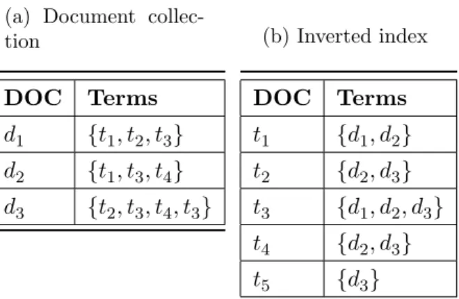
Imagine the collection DOC = {d₁, d₂, d₃} presented in Table 2.3(a), having only three documents with their respective terms. Table 2.3(b) shows the inverted index generated from the documents belonging toDOC. Observe that for each termt_i, the list of documents where it occurred is stored. For example, term t₁ occurred in documents

d₁ and d₂, term t₂ occurred in documents d₂ and d₃ and so forth.

After the indexation of the documents belonging to the collection, the retrieval pro-cess can be started. To perform a research, the user first specifies a query q_i, which reflects his/her need of information. Then the query q_i is processed together with the inverted index to retrieve a subsetD_j of all documents belonging to the collection.

The subset D_j contains only documents belonging to the collection that meets the restrictions imposed by the query performed by the user. Let us assume that q_i =

keyword:Database, so, set Dj corresponds to all documents of the database that

Basic Concepts 21

Table 2.3: Inverted Index example.

(a) Document collec-tion

DOC Terms

d₁ {t₁, t₂, t₃}

d₂ {t₁, t₃, t₄}

d₃ {t₂, t₃, t₄, t₃}

(b) Inverted index

DOC Terms

t₁ {d₁, d₂}

t₂ {d₂, d₃}

t₃ {d₁, d₂, d₃}

t₄ {d₂, d₃}

t₅ {d₃}

topics relevant to the information needed by the user, even though it does not satisfy directly the query performed. For example, for the query q_i, the system may return documents that do not have the term “database” but do mention “query processing” or “xml”.

The next stage of the process of information retrieval is to rank the result obtained, presenting to the user an ordered list of documents according to the relevance presented in the query that was performed. Different metrics may be used to rank documents according to a specific query, such as the vector space model (Lee, Chuang & Seamons 1997),boolean model (Lee, Kim & Lee 1994),page ranking (Baeza-Yates & Davis 2004) and several probability models such as theProbability Latent Semantic Analysis (PLSA) (Hofmann 1999).

Chapter 3

Related Works

Over the years, different strategies have been started to integrate structured and textual data in OLAP analysis. They can be classified according to the way they build their textual hierarchies. There are many works using external knowledge resources and spe-cialists to build manually their textual hierarchy. Others adopt automatically hierarchy construction strategies.

Manual textual hierarchies: Text Cube (Lin, Ding, Han, Zhu & Zhao 2008) was the first work for building a textual hierarchy in OLAP technology. This work defines the term hierarchy as a tree where the root node has all the terms of all documents and the leaf nodes have a single term. Intermediate nodes are organized according to the semantics of lower level nodes. Tools like WordNet (Kilgarriff & Fellbaum 2000) can help the union of similar terms in each tree level. Important to notice that the hierarchy tree topology is manually built, including the number of levels in the tree.

Cube Index (Janet & Reddy 2010, Janet & Reddy 2011) adopt the Text Cube con-cepts to implement three indexes: next-word, directed and inverted indexes. Word and term have identical meaning in these works. The document hierarchy, presented in (Janet & Reddy 2011), does not specify any semantic relation among the terms, but rather a relation between a term and a document. The hierarchical document tree has exactly five levels: (i) word; (ii) word pair; (iii) sentence; (iv) paragraph; and (v) document.

In (Oukid, Asfari, Bentayeb, Benblidia & Boussaid 2013) a Text Cube approach based on contexts and named CXT-Cube is presented, in which each dimension is related to a contextual factor (Document context and User context). The authors proposed an aggregation operator, named OLAP rank (Orank), to aggregate a set of documents

24 Related Works

by ranking them in a descendant order using a vector space representation. CXT-Cube presented a new measure, where each document is represented by weighted vector, composed of the weight of the terms computed according to their occurrences and a relevance propagation method. The relevance propagation uses the concept hierarchy extracted from an external knowledge source, i.e., a domain ontology related to the dimension area.

There are many works in textual OLAP improving textual measures. They are normally based on Text Cube (Lin, Ding, Han, Zhu & Zhao 2008) concepts. The work (Ding, Zhao, Lin, Han, Zhai, Srivastava & Oza 2011) presented a solution for the problem of finding the top-k most relevant cells in a Text Cube, reducing the search space, estimating higher limits of relevance in order to explore the smallest number of cells to answer the query. The work (Zhang, Zhai & Han 2011) presented a new approach, named MicroTextCluster Cube (MiTexCube), that includes the concept of “micro-clusters” of documents as a compact representation of the document collection. The documents associated to each cube cell are grouped according to their similarities, where each cluster of documents is considered a pseudo-document. The works (Liu, Tang, Hancock, Han, Song, Xu, Manikonda & Pokorny 2012, Lee, Kim & Kim 2014) extend the Text Cube approach, developing more specialized measures to their areas of interest. In (Liu, Tang, Hancock, Han, Song, Xu, Manikonda & Pokorny 2012), the approach organizes social media data, generating a new measure named Human Social Cultural Behavior (HSCB), which performs a linguistic analysis in the documents. In the work (Lee, Kim & Kim 2014), it is adopted more popular Information Retrieval (IR) measures, such as term frequency-inverted document frequency (tf-idf) and Language Model (LM).

Topic Cube (Zhang, Zhai & Han 2009) presents an improvement of the Text Cube approach, using the concept of topics for the creation of textual hierarchy. The hierarchy no longer aggregates all the terms of the document collection, but only adds the topics that the user may be most interested in, offering a simpler and more accurate repre-sentation named topic hierarchy. Topic Cube adopts the Probabilistic Latent Semantic Analysis (PLSA) model (Hofmann 1999) to calculate the probability of each document belongs to a node of a previous defined topic tree.

Related Works 25

Han 2009) method for helping building automatic hierarchies. The hierarchy works for specific areas of the DBLP database and the hierarchy levels are known a priori, since they are extracted from an external knowledge source, but the levels associations in a hi-erarchy are built automatically using information network analysis. EventCube adopts

CATHY (Wang, Danilevsky, Desai, Zhang, Nguyen, Taula & Han 2013) method to build a topic hierarchy automatically.

In short, the literature presents strategies to manually and automatically build their topic hierarchies, however, all the studied approaches presented static topic hierarchies, that is, build only once and used by all the cube structure. DTCubing is the only approach that proposes the building of automatic and dynamic hierarchies, at each new cell of the data cube, in order to produce different and more relevant topics to the user.

As discussed in Section 2.4.1, automatic methods of topic hierarchization are ex-tremely sensitive to the number of terms, so, approaches which apply such methods opt for using only one text segment in the stage of building their topic hierarchy, the

title. DTCubing proposes the building of topic hierarchies from different segments (title,

abstract, keywords, etc.), in order to promote greater variety of topics to the user, since different text segments may have different topics.

Other limitation of the current textual OLAP is in the return of the multidimen-sional queries. Just like in the current Information Retrieval systems, the textual OLAP approaches found in the literature present a list of most relevant documents as a result of their multidimensional queries. Because it uses different text segments to build its hierarchies, DTCubing presents a list of most relevant text segments as a result of its queries, facilitating the user’s final process of analysis.

Table 3.1 presents a comparison between the approaches found in the literature with DTCubing following the four main characteristics discussed in this Chapter: Automatic Hierarchies,Dynamic Hierarchies, Hierarchies built for multiple text segments and mul-tiple segment rankings as return of a multidimensional query.

26 Related Works

Table 3.1: Comparison of literature approaches with DTCubing

Approach Automatic Hierarchy

Dynamic Hierarchy

Hierarchies by Segments

Multiple Segmented Rankings

TextCube × × × ×

Cube Index × × × ×

CXTCube × × × ×

TopCells × × × ×

MiTexCube × × × ×

SocialCube × × × ×

TopicCube × × × ×

iNextCube × × × ×

EventCube X _{× × ×}

Chapter 4

DTCubing Approach

In this Chapter, the DTCubing approach is described in details. Section 4.1 presents the concept of text segments, used in the building of topic hierarchies. Section 4.2 presents the formal definition of a DTCubing cube, as well as the DTCubing cell and measure. Finally, Section 4.3 details the topic hierarchies built in DTCubing.

4.1

Text Segments

A text segment can be defined as any set of subsequent terms belonging to a document, following a pattern for its structuring. In a collection formed by scientific articles, for example, each document (i.e., article) can be segmented into smaller units, such astitle,

abstract, sentence, paragraph or any other type of segmentation desired. Each unit of representation of a document can be defined as text segment. It is possible to notice that an equivalence relation between two sets of segments where the union of the terms of each set separately corresponds to the same final content. The union of all paragraphs of a document must be equivalent to the union of all sentences in this document, considering that both segments represent the same term’s set, since all sentences are present in some of the paragraphs. One-time segments are named unique segments, such as scientific article’stitle or abstract.

28 DTCubing Approach

4.2

Data Cube and Cube Cell Concepts

A data cube is composed of base cells and aggregate cells. A multidimensional aggre-gate cell contains at least one dimension attribute value that equals ALL(*). A base cell contains only attribute values different from ALL. The ALL wildcard represents all attribute values of a specific dimension attribute. In range cubes (Silva, Hirata & de Castro Lima 2015), the wildcard ALL can represent some attribute values, so a single wildcard is not enough for full range cubes.

DTCubing is composed of structured dimensions, topic hierarchies and ranking mea-sures. It also has base cells and aggregate cells, but the ALL is adopted only in structured dimensions, producing a lattice of cuboids in the same way a traditional and structured data cube does. Bottom up, top down or hybrid computations can be performed in the same way they occur in non-textual OLAP.

A DTCubing DT C = {D₁, D₂, ..., D_n, T, R} where D_i is the i-th structured dimen-sion in a data cube. A dimendimen-sion D_i is composed of multiple hierarchies, so D_i =

{{A₁, A₂, A₄, ...},{A₃, A₅, ...}, ...,{A₁, A₃₄, ...}}orD_i ={{A₁, A₂, A₃, A₄, ..., A₃₄...}}, where each {A_i, A_j} is a hierarchy of a structured dimension of DTC (e.g., time dimen-sion composed of several attribute hierarchies {{year,month},{year,month,hour},. . .}). The dimension T = {DOC, T H₁, T H₂, ..., T Hn} is the text dimension, i.e., the

doc-ument collection DOC and all possible topic hierarchies {T H₁, T H₂, ..., T H_n}. R =

{R₁, R₂, ..., R_n}, stands for all possible rankings built in DTCubing where R_i refers to the ranking built from the T H_i hierarchy.

A DTCubing cell is represented asC = (a₁, a₂, a₃, ..., a_n,HS₁,HS₂, ...,HSm,R), where

each a_i is a structured attribute value of any dimension. Each a_i attribute value is associated with a unique dimension. Each DTCubing cell aggregates a text segments’ set{[S1],[S2], ...,[Sm]}obtained from DOC and presented hierarchically , where eachHSi

is the topic hierarchy built from the set of text segments [Si]. The set [Si] represents

the set of segments from the typei, which may be equal to abstract, reference,keyword,

sentence or title of a scientific article, for example. A DT C is composed of cells as any data cube.

Ris the C measure, composed of: {RS₁,RS₂, ...,RSm}, whereRSi is the i-th segment

ranking built from [Si] (e.g.,sentence ranking,title ranking,keyword ranking andabstract

DTCubing Approach 29

Each DTCubing hierarchy is a tree data structure, where each tree node is a distri-bution θ_j of topics. This way, HSi = {θ1, θ2, ..., θt}, where θj represents the j-th topic

distribution of HSi, and t is the number of nodes in HSi. Each distribution can be

represented as θ_j ={t₁, t₂, ..., t_z}, where each t_i represents a topic.

4.3

Multiple Topic Hierarchies per Cube Cell

Figure 2.7 of section 2.2 presents a good illustration of how the textual OLAP cubes cur-rently structured. Observe that the cube presents two structured dimensions (Conference and Time) and only one topic hierarchy, presented as a vertical dimension highlighted in red. Figure 4.1 below presents an illustration of the DTCubing cube for the same dimensions Conference and Time. Observe that now there is no longer that only topic hierarchy represented by the vertical axis. Now the hierarchies are dynamic and built at each new cell of the cube.

As a criterion of simplification, only the hierarchies of cells (Conference=SBSI,Year=

F EB98) and (Conference = J CIT,Year =F EB98) were illustrated, however, mul-tiple hierarchies are built for any other cell of the cube.

Figure 4.1: DTCubing approach

m Hierarquias SBSI JCIT JAN 99 FEB 99 JAN 98 FEB 98 Conference Tim e VLDB Hs1 Hs2

Hsm

Each DTCubing hierarchy is presented in the form of a tree, where each node is represented by a list of most relevant topics using the document collection of the topic tree. The topology of the tree can be specified according to the user’s need by updating the number of hierarchical levels.

30 DTCubing Approach

user. Let c_i be a specific data cube cell and Sci = {[S1],[S2], ...,[Sm]} the set of text

segments associated with this cell. Ifc_i were obtained from the queryq₁ = (Conference =

IJ CAI,Year = 2010), therefore containing filters only in the structured dimensions (Conference and Year, respectfully), DTCubing builds a topic hierarchy for each [Si] ∈

Sci that has no equivalence relation with any other set of segments. For those sets

that have an equivalence relation, only one set is selected, giving rise to one more topic hierarchy. As an example, the topic hierarchy for sentences would not be computed because the hierarchy for paragraphs has already been computed.

Formally, the setHci ={HS1, ...,HSk}represents theKhierarchies built forci, where

HSi is the hierarchy built from the text segments [Si]. The value K is always less than m because some of the segments of Sci are pruned. For the case where ci is obtained

from a query q₂ = (Conference = V LDB,Keyword = ”textual and spatial OLAP”), presenting a filter in the textual dimension, DTCubing builds a topic hierarchy for each [Si] ∈ Sc₁ without pruning. The difference is that only the segments that have the

Chapter 5

DTCubing Architecture

In this Chapter, the DTCubing Architecture is described in details. The DTCubing approach is partitioned into four steps: Indexing, Filtering, Hierarchy Generation and

Ranking. The solution computes range cubes, i.e., data cubes composed of cells that represent full or partial aggregations, so the traditional ALL value exists, but also several other partial ALL values, originated from filters, such as between, similar, less than,

some, contains and many more. The exponential behavior turns impractical full range cube strategies.

Supose anABC relation with cardinalitiesC_A,C_B andC_C equal to 2. Only with this small relation, there are (C_A+ 1)×(C_B+ 1)×(C_C+ 1) = 27 tuples in a traditional full data cube. These tuples can be represented as t1 = (A₁, B₁,∗, m), t2 = (A₂, B₁,∗, m),

t3 = (A₁, B₂,∗, m), t4 = (A₂, B₂,∗, m), t5 = (A₁,∗, C₁, m), ..., t27 = (∗,∗,∗, m), onde

A₁,A₂,B₁,B₂,C₁ andC₂ are dimension attributes, m is a numerical value representing a measure and ”*” is a wildcard representing all values of a cube dimension.

Now consider a new wildcard ”**” representing two attributes of one same dimension, enabling tuples in the form t28 = (A₁A₂, B₁, C₁, m),t30 = (A₁, B₁B₂, C₁, m) and many others. Instead of ((C_A+1)×(C_B+1)×(C_C+1) computed tuples, a range cube can have 2CA_×2CB _×2CC _{tuples. In our example, the range cube would have 2}2_×22_×22 _{= 64}

tuplas from the ABC relation. This behavior can be better detailed in (Silva, Hirata & de Castro Lima 2015, Silva, Hirata & de Castro Lima 2016).

The four steps of DTCubing algorithm are organized as Figure 5.1 illustrates. Ini-tially, the input document collection is traversed and indexed by the Indexing step, resulting in the 1D-cuboid, i.e., all the dimensions are aggregated individually. The

32 DTCubing Architecture

Indexing step is only performed again if there is a relation update, otherwise, it is only executed once.

Figure 5.1: DTCubing Architecture steps

Document Collection

Indexing Dimension A TIDs

Dimension B TIDs

Dimension n TIDs

Partial Cubes

Filtering

Fill = {f1, f2, ..., fn}

Result Cells

C = {[S ], [S ], ..., [S ]}i 1 2 m

Hierarchy Generation {H , Hs1 s2, ...,Hsp}

θi,j

Ranking

Start

Finish

Hsj [C C1, 2, ...,C ]n

AfterIndexing the partial cubes, it is possible to perform the other steps repeatedly, where the iterative behavior is illustrated by the dashed arrows of Figure 5.1. The

Filtering step starts with the definition of a set of filters F il={f₁, f₂, ..., f_n}applied to the dimensions of the cube. In response to this step, a set namedresultCells is obtained, containing all the cube cells that meet the restrictions imposed by the application of the filters.

For the next step to be started, the user must select one of the cells ([c₁, c₂, , ..., cn])

returned by theFiltering step. Each cell returned by the Filtering has a set of text seg-ments {[S1],[S2], ...,[Sm]}, so in Hierarchy Generation step a hierarchy is built for each

set of segments associated with the selected cell, originating the set {HS1,HS2, ...,HSp},

wherep=m if there is at least one filter applied to the textual dimension orp < m oth-erwise. The last step starts when the user selects a nodeθ_j from hierarchyHSi, starting

the Ranking step. The Ranking step presents thetop-k text segments most relevant to the user. After theRanking step, the user can start a new query pipeline or return to a previous step. In the next sections, the algorithms that make up each step are detailed.

5.1

Indexing

In the Indexing step a document collectionDOCis defined as a set of tuples, where each tuplet is formalized ast= (T ID, D₁, D₂, ..., Dn, doc1, doc2, ..., docd), wheren is equal to

DTCubing Architecture 33

Table 5.1: Indexing Step example.

(a) Document collection

TID A B C DOC

1 a1 b1 c1 doc₁ ={w₁, w₂, w₃}

2 a1 b2 c2 doc₂ ={w₂, w₃}

3 a2 b2 c3 doc₃ ={w₃, w₄, w₅}

4 a3 b3 c3 doc₄ ={w₁, w₂, w₅}

(b)dtc- Partial Cube

Att Values TIDs List

a1 1,2

a2 3

a3 4

... ...

c3 3,4

w_{1 1,4}

w_{2 1,2,4}

w_{3 1,2,3}

w_{4 3}

w_{5 3,4}

tuplet. Each structured dimension is in the formD_j ={at_1,j+at_2,j+...+at_C,j}, where

C is the cardinality of the dimension and at_i,j corresponds to the i-th attribute of the dimension j. The symbol + corresponds to the logical operator OR. T ID corresponds to a single identifier, ensuring that there is no other equal tuple in DOC.

Table 5.1 presents an example of the Indexation process in DTCubing. The DOC

collection illustrated in Table 5.1(a) is used as input for the Indexing process, which produces as output a data cube in the form dtc = (...(iT_at

1,j, iTat2,j, ..., iTatn,j)..., T, R)

represented in table 5.1(b). Each internal element (iT_at

1,j, iTat2,j, ..., iTatn,j) corresponds

to the set of inverted tuples of a specific dimension. EachiT_at

1,j = (ati,j, T ID1, ..., T IDP)

represents the inverted list of tuples of the attributeat_i,j, storing a set of tuple identifiers (T ID₁, ..., T ID_P), representing the P occurrences of at_i,j in DOC.

For example, the attribute a1 presented in Table 5.1(a) occurred in tuples 2 and 3, whereas the attributea2 occurred only in tuple 3, and so on. Observe that when reaching the textual dimension, its documents are only broken in terms and indexed in the same manner as the structured attributes Considering the document terms as attributes and storing them individually in an inverted index facilitates the application of filters such as ends-with,different, contains or similar in the textual dimension.

34 DTCubing Architecture

the text segments considered, as described in Section 4.2.

The Algorithm 5.1 presents the routine of the Indexing step implemented in this work. The variable sortedC (line 1) stores the cardinality of each dimension, useful for optimize the aggregations computation in the subsequent steps. The variableinvertedT

(line 2) stores all the attributes ofDOC, as well as theirT ID lists. Besides the attributes of the structured dimensions, document terms of each tuple are also indexed and stored ininvertedT.

Algoritmo 5.1: Indexing Step Algorithm

input:DOC int[]sortedC;

1

M aphatt, SethT IDii[]invertedT;

2

M aphdocID, segmentsi[]S;

3

while DOC has tuples do 4

i= 1;

5

tuple t = DOC.tuples;

6

while t has dimensions do 7

if t.dimension.isStructured() then 8

update or create new entrance in invertedT for each attribute;

9

else 10

d = removeStopWords(t.getDoc());

11

segments = splitSegments(d);

12

S.put(i, segments);

13

i+ +;

14

foreach term in d do 15

update or create new entrance in invertedT for each term;

16

update sortedC to mantain dimensions according to their cardinalities;

17

returndtC;

18

DTCubing Architecture 35

attribute at_i has been read for the first time, a new input is created in the variable

invertedT. Otherwise, the T ID list of at_i is updated with a new occurrence. When it is a textual dimension, the algorithm removes the stopWords from each document (line 11), separating its text segments (line 12) and adding them to the variable S (line 13). In sequence, the algorithm indexes all the document terms, as it does for the structured dimensions (lines 15-16).

5.2

Filtering

The Filtering step in DTCubing covers the application of point filters, range filters and a combinatorial filter, named inquire (Silva, Lima & Hirata 2013, Silva, Hirata & de Castro Lima 2015, Li, Han & Gonzalez 2004). In this step, the user selects the cells that are used for the topic hierarchies building. A point filter has only the equality operator. A range filter can be classified in: greater than, less than, between, different,

contains, some and similar. All the range filters include the attribute ALL in its result. Lastly, an inquire filter has only one operator that gathers all the attribute values of a dimension plus ALL, resulting in a sub-cube. One or more cube cells are obtained from the Filtering step.

The Algorithm 5.2, presented for the Filtering process in DTCubing, has as input the partial cube dtc, obtained from the Indexing step, and the set F il ={f₁, f₂, ..., fn}

of filters defined by the user. Each filter f_i ∈ F il is applied to a specific dimension of the cube, so the algorithm first obtains the attribute values of each dimension, storing them in the variableattValues (lines 3-5).

Suppose that the set of filters applied is the set F il : (Author = J iawei Han, Conference=ALL, Ano= 2014−2017,Keyword≈“OLAP”). Table 5.2 corresponds to the values of attributes obtained from each dimension that meet the restrictions of the filters contained in F il.

After defining the attribute values of each dimension, the algorithm produces all the possible aggregations with the values contained in attValues (line 6). Table 5.3 corresponds to all possible aggregations formed with the values of attributes present in Table 5.2.