http://dx.doi.org/10.1590/S1982-21702013000300006
ROBUSTNESS ANALYSIS OF GEODETIC NETWORKS IN
THE CASE OF CORRELATED OBSERVATIONS
Analise de Robustez de redes Geodésicas para o caso de observações correlacionadas
MEVLUT YETKIN1 MUSTAFA BERBER2
CEVAT INAL3
1
Department of Geomatics Engineering, Izmir Katip Celebi University, Balatcik Campus, Izmir, 35620, Turkey
2
Department of Civil, Environmental and Geomatics Engineering, Florida Atlantic University, 777 Glades Road, Boca Raton, FL, USA, 33431
3
Department of Geomatics Engineering, Selcuk University, Alaaddin Keykubad Campus, Konya, 42250, Turkey
ABSTRACT
normalized reliability numbers are small, displacements get large, i.e., observations with low reliability numbers cause bigger displacements compared to observations with high reliability numbers.
Keywords: Robustness; Strain; Displacement; Reliability; GPS Network.
RESUMO
Redes GPS (ou GNSS) são ferramentas valorosas para monitorar desastres naturais, tais como terremotos. No entanto, erros nas observações GPS podem ser erroneamente interpretados como deformação. Portanto, redes robustas são necessárias no monitoramento de deformação. Análise de robustez é uma fusão de confiabilidade e de tensão e definida como a capacidade de resistir as deformações causadas pelos erros máximos não detectáveis, tal como é determinado a partir de análise de confiabilidade interna. Para obter resultados rigorosamente corretos, no entanto, as correlações entre as observações devem ser consideradas ao calcular erros máximos não detectáveis. Assim, propõe-se utilizar os números de confiabilidade normalizados em vez de números de redundância (abordagem de Baarda) na análise de robustez de uma rede GPS. Uma relação matemática simples que mostra a razão entre os casos não correlacionados e correlacionados para o erro máximo não detectável é derivada. A mesma razão também é válida para os deslocamentos. Os resultados numéricos mostram que se as correlações entre as observações são ignoradas, diferentes deslocamentos podem ser obtidos, dependendo da dimensão dos múltiplos coeficientes de correlação. Além disso, quando os números de confiabilidade normalizados são pequenos, são obtidos grandes deslocamentos, ou seja, observações com números baixos de confiabilidade causam deslocamentos maiores em comparação com observações com números elevados de confiabilidade.
Palavras-chave: Robustez; Retas; Deslocamento; Confiabilidade; Rede GPS.
1. INTRODUCTION
used to calculate its vital characteristics including details about the fault rupture. Accurate and rapid identification of earthquakes is crucial for disaster response and mitigation efforts(HU et al., 2005; HASHIMOTO et al., 2006; SNAY and SOLER, 2008; LIM et al., 2010).
Using GNSS measurements of ground displacements, the time needed to locate and characterize the damage might be reduced. In order to be able to that crustal strain may be determined by finding the relative displacements between GNSS stations. In other words, GNSS measurements are used to observe ground movement and strain. Strain is defined as the ratio of increase in length to its original length and strain analysis has been used with geodetic networks in the past. Here, the length means the distances or connections between reference sites. One example of use of strain analysis with geodetic networks is robustness analysis (VANÍČEK et al., 1991; KRAKIWSKY et al., 1993; VANÍČEK et al., 2001; HSU and LI, 2004; BERBER, 2006; BERBER et al., 2006; BERBER et al., 2008; HSU et al., 2008; VANÍČEK et al., 2008; YETKIN, 2012; YETKIN and BERBER, 2013). In robustness analysis, strain analysis is used to portray the effect of undetected errors because strain technique is independent of adjustment constraints and reflects only the network geometry and accuracy of the observations(BERBER, 2006). One thing must be clarified at this point that in robustness analysis a virtual displacement (potential deformation that could be introduced by the undetected errors in the observations and this is considered as a kind of potential ‘displacements’) is examined.
To measure robustness of a network, displacements of individual network points are portrayed by strain. This technique is known as robustness analysis (BERBER et al. 2009). Robustness analysis has two building blocks; one is reliability analysis and another is strain analysis. Reliability theory that is developed by Baarda (1968) is based on the assumption that observations are uncorrelated. Nevertheless, correlated observations are very often encountered in geodesy; for instance, simultaneously observed baseline vectors in GPS campaigns are correlated. Therefore, neglecting correlations among the observations may falsify the results in a reliability analysis. Reliability analysis can be separated into two as internal and external reliability. A good and homogeneous internal reliability does not automatically guarantee reliable coordinates of network points. Thus, the effects of undetectable errors on the parameters are to be estimated by external reliability. However, external reliability criterion depends on the definition of internal reliability meaning that if internal reliability is defined for correlated observations, the external reliability and therefore robustness analysis will yield different results.
to redundancy numbers (Baarda’s approach) that are only valid for uncorrelated observations. They are called normalized reliability numbers and lie in the interval of [0,1].
In the case of correlated observations, internal reliability is calculated using normalized reliability numbers and this is substituted into external reliability equation. Thus, strain matrix at each point of the network is obtained by considering the correlations. Then, following the procedure outlined in Berber (2006) displacements of network points are obtained. In this study, maximum undetectable errors for correlated observations are incorporated and using them robustness analysis is performed.
2. ROBUSTNESS ANALYSIS
The maximum undetectable errors in observations which would not be detected by a statistical test is given by Baarda (1968) as
i i 0 i
r
l
=
δ
σ
Δ
(1)where
δ
0 is the lower bound for the non-centrality parameter that is a function of Type I and II errors. The value of the non-centrality parameter depends on the levels of probability assumed for the data snooping procedure, i.e., the chosen probability levels for decision errors affect the non-centrality parameter. As well known, it is possible to commit two kinds of decision errors when using statistical tests. Rejecting an unbiased observation as one that is biased is called a Type I error. On the other hand, accepting a biased observation as an unbiased one is called a Type II error (GHILANI and WOLF, 2010).σ
iandr
i are the standard deviation and redundancy number of the ith observation respectively. The maximum undetectable errors constitute the internal reliability of the network. The following development was originally reported in Berber et al. (2009).In addition, the interested reader is referred to Vaníček et al., (1991); Berber, (2006); Vaníček et al., (2008) and Hsu et al., (2008) for further information about 3D robustness analysis. The least squares estimate for the displacementsΔ
x
caused by the maximum undetectable errorsΔ
l
in the observations is given by(
)
-1 Δl=
Δx ATPA ATP (2)
reflects only the network geometry and accuracy of observations. Here robustness analysis is given in general form in 3D. However, 1D and 2D cases are also investigated in Berber (2006). Let us consider the 3D displacements of a point P by
⎥ ⎥ ⎥ ⎦ ⎤ ⎢ ⎢ ⎢ ⎣ ⎡ = ⎥ ⎥ ⎥ ⎦ ⎤ ⎢ ⎢ ⎢ ⎣ ⎡ Δ Δ Δ = Δ i i i i i i i w v u z y x x (3)
Then, the gradient with respect to position is
⎥ ⎥ ⎥ ⎥ ⎥ ⎥ ⎥ ⎦ ⎤ ⎢ ⎢ ⎢ ⎢ ⎢ ⎢ ⎢ ⎣ ⎡ ∂ ∂ ∂ ∂ ∂ ∂ ∂ ∂ ∂ ∂ ∂ ∂ ∂ ∂ ∂ ∂ ∂ ∂ = z w y w x w z v y v x v z u y u x u i i i i i i i i i i E (4)
For
∀
j
=
0,1,…,t (t is the number of connections) the displacements u, v and w are calculated as follows:(
)
(
)
(
)
(
)
(
)
(
)
(
)
(
)
(
j i)
ji i j i i j i i j i j i i j i i j i i j i j i j i i j i i Z Z z w Y Y y w X X x w c Z Z z v Y Y y v X X x v b Z Z z u Y Y y u X X x u a w v u i = − ∂ ∂ + − ∂ ∂ + − ∂ ∂ + = − ∂ ∂ + − ∂ ∂ + − ∂ ∂ + = − ∂ ∂ + − ∂ ∂ + − ∂ ∂ + (5)
where all the partial derivatives as well as the absolute terms ai ,bi and ci and the coordinates Xi,Yi and Zi refer to point P , and P is connected (by an observation) to the point of interest, point P . In matrix form:
i
(
)
(
)
(
)
iT T T T T T w Q K K K v Q K K K u Q K K K i i 1 i i i i i i i i i 1 i i i i i i i i i 1 -i i i i i i z w y wx w c , z v y v x v b , z u y u x u a = = ⎥ ⎥ ⎥ ⎥ ⎥ ⎥ ⎥ ⎦ ⎤ ⎢ ⎢ ⎢ ⎢ ⎢ ⎢ ⎢ ⎣ ⎡ ∂ ∂∂ ∂∂ ∂ = = ⎥ ⎥ ⎥ ⎥ ⎥ ⎥ ⎥ ⎦ ⎤ ⎢ ⎢ ⎢ ⎢ ⎢ ⎢ ⎢ ⎣ ⎡ ∂ ∂∂ ∂∂ ∂ = = ⎥ ⎥ ⎥ ⎥ ⎥ ⎥ ⎥ ⎦ ⎤ ⎢ ⎢ ⎢ ⎢ ⎢ ⎢ ⎢ ⎣ ⎡ ∂ ∂∂ ∂∂ ∂ − − (6)
Assembling them into a hypermatrix and using Eq. (4), we get
i
∀
in the network( )
⎥ ⎥ ⎥ ⎦ ⎤ ⎢ ⎢ ⎢ ⎣ ⎡ ⎥ ⎥ ⎥ ⎦ ⎤ ⎢ ⎢ ⎢ ⎣ ⎡ = i i i i i i i 0 0 0 0 0 0 w v u Q Q Q Evec (7)
The
Q
i matrix is formed by eliminating the first row of the matrix(
T)
TK
K
K
i i −1 i in Eq. (6). If we show the reduced matrix with T and substitute Eq. (3) in Eq. (7)we reachi
∀
in the network( )
E
iT
ix
ivec
=
Δ
(8)Substituting Eq. (2) in Eq. (8), we write
i
∀
in the network( )
E
i=
T
i(
A
PA
)
−1A
P
Δ
l
In a 3D network, the dimensions of the , and matrices are 1 ,
1 and 9 , respectively. As mentioned earlier, is the number of connections.
The displacements can be computed using the elements of strain matrix E . However, first “initial conditions” X0, Y0 and Z0 must be determined to be able to compute displacements induced by the maximum undetectable errors. In other words, displacements are calculated from a system of first order differential equations, and these equations should be integrated to solve them. Therefore, initial conditions are needed (BERBER 2006). Initial conditions are the coordinates that are obtained minimizing the norm of displacement vector at all points in the network. This means that to calculate X0, Y0 and Z0, the displacements in the network points should be minimized and this is explained in Berber et al. (2009). Once X0, Y0 and Z0 have been determined ui,vi and wi are calculated from:
⎥
⎥
⎥
⎦
⎤
⎢
⎢
⎢
⎣
⎡
−
−
−
⎥
⎥
⎥
⎥
⎥
⎥
⎥
⎦
⎤
⎢
⎢
⎢
⎢
⎢
⎢
⎢
⎣
⎡
∂
∂
∂
∂
∂
∂
∂
∂
∂
∂
∂
∂
∂
∂
∂
∂
∂
∂
=
⎥
⎥
⎥
⎦
⎤
⎢
⎢
⎢
⎣
⎡
0 i 0 i 0 i i i i i i i i i i i i iZ
Y
Y
X
X
z
w
y
w
x
w
z
v
y
v
x
v
z
u
y
u
x
u
w
v
u
Z
(10)In robustness analysis, one moves from displacement field to strain field by using strain analysis. Thus, the elements of the strain matrix can be obtained. However, some threshold values are needed to assess the network robustness. So, one has to return from strain field to displacement field in order to obtain displacement values of the points. This is realized by Eq. (10). Unlike displacements obtained by external reliability values, displacements obtained from robustness analysis that is a purely geometrical approach are strain based and they can be compared with threshold values to assess the robustness of the network (BERBEr, 2006).
After computing the displacements u,v and w for each point in the network, we obtain the amount of total displacement at each point from:
2 i 2 i 2 i
i
u
v
w
d
=
+
+
(11)3. RELIABILITY MEASURES FOR CORRELATED OBSERVATIONS
As it is well known, the redundancy numbers of the observations
( )
r
i are the diagonal elements of the matrix R(
A PA)
A P AI
R = − T −1 T (12)
where I is the identity matrix. In the case of uncorrelated observations, they lie between 0 and 1 (BAARDA (1967) and (1968)):
1
r
0
≤
i≤
(13)If the observations are correlated, the redundancy numbers are no longer bound to the interval of [0,1] and may even be negative. Therefore, Wang and Chen (1994) introduced the reliability numbers
r
i as follows:i i
i 1 i
i
h
h
h
h
r
=
TP
− TPQ
vP
(14)where
h
i is an n by 1 vector containing zeros with a one corresponding to an observation. The bounds of these reliability numbers are(
2)
1i i
1
r
0
≤
≤
−
ρ
− (15)where
ρ
i is the multiple correlation coefficient and is defined by( ) ( ) ( )
1
0
,
q
2 i ii
i -1
ii i 2
i
=
≤
ρ
<
ρ
q
Q
q
T
(16)
where the
(
n
−
1
)
×
1
vectorq
( )i corresponds to the ith column of1
−
=
P
Q
after(
2)
i i i
r
1
r
=
−
ρ
(17)The interpretation of the normalized reliability numbers and their possible application to reliability investigations is similar to that of the ordinary redundancy
numbers. This means that
r
j=
0
indicates an uncontrolled observation, while1
r
j=
indicates an unnecessary one (WIESER 2002).If the observations are correlated, no change of Eq. (2) is required, but obviously, Eq. (1) is invalid. In this case, the maximum undetectable errors are computed using the normalized reliability numbers as follows:
i ii
0 0 i
r
l
p
σ
δ
=
Δ
(18)where
p
ii is the ith diagonal element of the matrix P (Schaffrin 1997).4. EVALUATION OF STRAIN MATRIX IN THE CASE OF CORRELATED OBSERVATIONS
As it is mentioned in section 2, robustness analysis uses Baarda’s external reliability criterion as the local displacement field. This means that the computation of maximum undetectable errors in Eq. (1) and consequently the external reliability vector in Eq. (2) assumes uncorrelated observations for which the covariance matrix is diagonal. Realistically; however, one must consider the correlations among the observations in many applications such as GPS networks. Thus, the elements of the strain matrix must be computed by using maximum undetectable errors that are computed with the normalized redundancy numbers as seen in Eq. (18). 9. On the other hand, a general expression for maximum undetectable errors can be seen in Teunissen (2000). Then the strain matrix at each point can be obtained using the equation below
( )
E
i=
T
i(
A
PA
)
−1A
P
Δ
l
vec
T T (19)5. RELATIONSHIP BETWEEN THE UNCORRELATED AND CORRELATED CASES
Let us consider the ratio of Eq. (1) to Eq. (18) (in Eq. 18
σ
0 is considered 1). Then we have2 i ii i i i i i ii 0 i ii i i 0 i i
p
r
r
r
r
p
r
p
r
l
l
σ
=
σ
=
δ
σ
δ
=
Δ
Δ
(20)which in combination with Eq. (17) yields
(
)
i i 1 2 i ii 2 i i i i ir
r
p
1
r
r
l
l
=
−
ρ
σ
=
Δ
Δ
43
42
1
(21)and with
r
i=
r
i(
1
−
ρ
i2)
we obtain(
)
2i i i 2 i i i i i
1
1
r
r
1
r
r
l
l
ρ
−
=
ρ
−
=
Δ
Δ
(22)As can be seen with the equation above, as the value of
ρ
i increases, thedifference between
Δ
l
i which is based onr
i andΔ
l
i which is based onr
i increases as well. This indicates that while doing the reliability analysis, the correlations must be taken into account. Similarly, since the same parameters are used for robustness, the results of robustness analysis change accordingly.6. NUMERICAL RESULTS
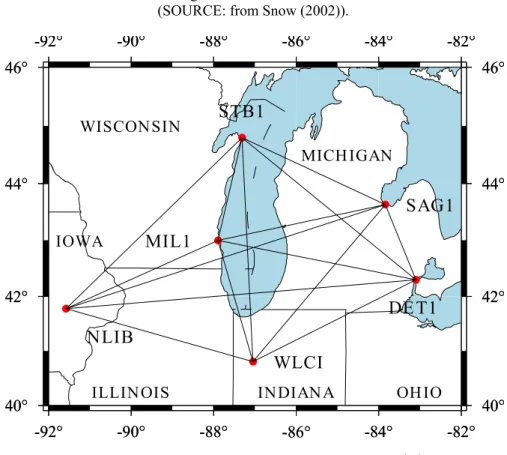
A GPS network example given in Snow (2002) is used to test the proposed approach. The network consists of 6 Continuously Operating Reference Stations (see Figure 1). There are a total of 15 measured baseline vectors. The variance-covariance matrix for this GPS network is a block-diagonal type, with an individual
Figure 1 - GPS network . (SOURCE: from Snow (2002)).
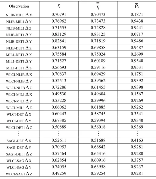
Redundancy numbers
( )
r
i , normalized reliability numbers( )
r
i and multiple correlation coefficient( )
ρ
i values can be obtained from Eqs. (12), (17) and (16) respectively. These values are shown in Table 1. The range of multiple correlation coefficients is 0.0717-0.9540.Maximum undetectable errors are calculated for both using redundancy numbers (Eq. 1) and normalized reliability numbers (Eq. 18), and their ratios are shown in Table 2.
As can be seen in Table 1 and 2, while the ratio of
Δ
l
iΔ
l
i is small (around1) for the observations whose
ρ
i values are close to 0, the ratio ofΔ
l
iΔ
l
i islarger for the observations whose
ρ
i values are close to 1. The reason behind these patterns is explained in the last paragraph in section 5.-92° -92°
-90° -90°
-88° -88°
-86° -86°
-84° -84°
-82° -82°
40° 40°
42° 42°
44° 44°
46° 46°
-92° -92°
-90° -90°
-88° -88°
-86° -86°
-84° -84°
-82° -82°
40° 40°
42° 42°
44° 44°
46° 46°
DE T1
MIL1
NLIB
SAG1
STB1
WLCI
IOWA
WISCON SIN
ILLIN OIS IN DIAN A OH IO
Table 1 - Redundancy numbers, normalized reliability numbers and multiple correlation coefficients. Only first 6 and last 2 baselines are shown to keep the table
brief.
Observation
r
ii
r
ρ
iNLIB-MIL1
Δ
X 0.70791 0.70473 0.1871NLIB-MIL1
Δ
Y 0.76962 0.73473 0.9438NLIB-MIL1
Δ
Z 0.71555 0.72828 0.9441NLIB-DET1
Δ
X 0.83129 0.83125 0.0717NLIB-DET1
Δ
Y 0.82841 0.71819 0.9486NLIB-DET1
Δ
Z 0.63159 0.69858 0.9487MIL1-DET1
Δ
X 0.75584 0.75024 0.2699MIL1-DET1
Δ
Y 0.71527 0.60189 0.9540MIL1-DET1
Δ
Z 0.56693 0.59116 0.9531WLCI-NLIB
Δ
X 0.70837 0.69429 0.1751WLCI-NLIB
Δ
Y 0.52513 0.59562 0.9392WLCI-NLIB
Δ
Z 0.72286 0.61455 0.9398WLCI-MIL1
Δ
X 0.49530 0.49604 0.1567WLCI-MIL1
Δ
Y 0.55228 0.59996 0.9269WLCI-MIL1
Δ
Z 0.66062 0.61885 0.9262WLCI-DET
Δ
X 0.60443 0.58745 0.3541WLCI-DET
Δ
Y 0.67385 0.59394 0.9340WLCI-DET1
Δ
Z 0.50889 0.56018 0.9369M
M
M
M
SAG1-DET
Δ
X 0.52611 0.51688 0.4163SAG1-DET
Δ
Y 0.70953 0.66842 0.9281SAG1-DET1
Δ
Z 0.57464 0.65316 0.9280WLCI-SAG
Δ
X 0.62854 0.60916 0.3757WLCI-SAG
Δ
Y 0.74055 0.63958 0.9237Table 2 - Maximum undetectable errors (m). Only first 6 and last 2 baselines are shown to keep the table brief.
Observation
Δ
l
iΔ
l
ii
i
l
l
Δ
Δ
NLIB-MIL1
Δ
X 0.0017 0.0017 1.02NLIB-MIL1
Δ
Y 0.0074 0.0025 2.96NLIB-MIL1
Δ
Z 0.0068 0.0022 3.06NLIB-DET1
Δ
X 0.0024 0.0024 1.00NLIB-DET1
Δ
Y 0.0075 0.0026 2.94NLIB-DET1
Δ
Z 0.0073 0.0022 3.33MIL1-DET1
Δ
X 0.0017 0.0016 1.03MIL1-DET1
Δ
Y 0.0060 0.0020 3.06MIL1-DET1
Δ
Z 0.0058 0.0017 3.37WLCI-NLIB
Δ
X 0.0017 0.0017 1.00WLCI-NLIB
Δ
Y 0.0070 0.0022 3.10WLCI-NLIB
Δ
Z 0.0055 0.0020 2.70WLCI-MIL1
Δ
X 0.0010 0.0010 1.01WLCI-MIL1
Δ
Y 0.0053 0.0019 2.78WLCI-MIL1
Δ
Z 0.0044 0.0017 2.57WLCI-DET
Δ
X 0.0014 0.0013 1.05WLCI-DET
Δ
Y 0.0053 0.0020 2.63WLCI-DET1
Δ
Z 0.0051 0.0017 3.00M
M
M
M
SAG1-DET
Δ
X 0.0015 0.0014 1.09SAG1-DET
Δ
Y 0.0056 0.0021 2.61SAG1-DET1
Δ
Z 0.0052 0.0018 2.86WLCI-SAG
Δ
X 0.0014 0.0013 1.06WLCI-SAG
Δ
Y 0.0050 0.0021 2.43WLCI-SAG1
Δ
Z 0.0051 0.0017 2.95Table 3 shows the displacements at each network point, that are obtained from Eq. (11) for
δ
0(
α
0=
5
%,
β
0=
5
%
)
=
3
.
61
. The displacements obtained usingTable 3 - Displacements of network points (mm).
Site
d
ii
d
MIL1 0.8295 0.2675 WLCI 1.1554 0.4372 NLIB 1.7915 0.5777 STB1 0.8944 0.3776 SAG1 0.9206 0.2848
As can be seen in Table 3, when the correlations are considered, the displacement values are different from the displacement values for the uncorrelated cases. This is because, in the network used as an example, some
ρ
i values are quite high. Thus, when robustness analysis is applied to correlated observations, for rigorous results the correlations among observations must be taken into account.In order to be able to show the importance of
ρ
ion robustness analysis, twoobservations (MIL1-DET1 whose
ρ
i=0.9540 and WLCI-NLIBwhose
ρ
i=0.0717-these are the observations with highest and the lowest multiple correlation coefficients) are considered and displacement values are computed and these are listed in Table 4 and 5 respectively. Needless to say while calculatingd
ivalues,
ρ
i are ignored andr
i values are used. The ratio of displacement is biggerfor the observation whose
ρ
i is large. Whereas, as one would expect, the ratio ofdisplacements is 1 for the observation whose
ρ
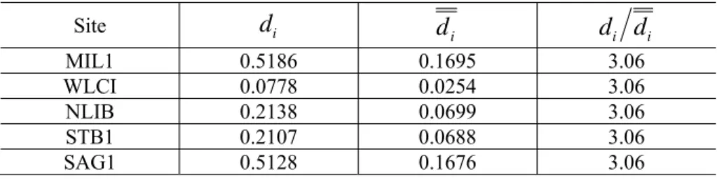
i is close to 0. In addition, the ratio of the displacement for the same observation is the same as the ratio of the maximum undetectable errors in Table 2. Similar results have been obtained for other observations.Table 4 - Displacements due to MIL1-DET1 -(mm).
Site
d
id
id
id
iMIL1 0.5186 0.1695 3.06 WLCI 0.0778 0.0254 3.06 NLIB 0.2138 0.0699 3.06 STB1 0.2107 0.0688 3.06 SAG1 0.5128 0.1676 3.06
( )
Δ
Y
( )
Δ
X
Table 5 - Displacements due to NLIB-DET1 -(mm).
SITE
d
id
id
id
iMIL1 0.0863 0.0861 1.00 WLCI 0.0528 0.0527 1.00 NLIB 0.2018 0.2013 1.00 STB1 0.0417 0.0416 1.00 SAG1 0.1355 0.1352 1.00
To show the relationship between reliability and robustness, let us assume an
observation whose all elements of
Δ
l
i except forr
i are 1. By doing this, we can clearly observe the effect of normalized reliability numbers on displacements. Thedisplacements are computed for two extreme cases, i.e.,
r
i=
0
.
9999
and0001
.
0
r
i=
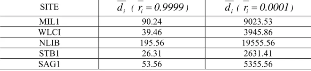
. Maximum undetectable error corresponding to these normalized reliability numbers are computed using Eq. (18) as 1 m and 100 m respectively. The displacements of network points are shown in Table 6.Table 6 - Displacements for two extreme cases (mm).
SITE
i
d
(r
i=
0
.
9999
)d
i (r
i=
0
.
0001
)MIL1 90.24 9023.53 WLCI 39.46 3945.86 NLIB 195.56 19555.56 STB1 26.31 2631.41 SAG1 53.56 5355.56
As seen from Table 6, very big displacements are obtained for low reliability numbers as opposed to the displacements for high reliability numbers. These displacements with low reliability numbers are 100 times bigger than their counterparts with high reliability numbers. This is because the ratio between the highest and lowest reliability numbers is 10,000. Since the other elements are neutral, this ratio between high and low reliability numbers is directly reflected to the displacements. As reliability numbers decrease as shown above, maximum undetectable errors increase and this cause larger displacements at network points. Seemkooei (2001a) and Seemkooei (2001b) have reported that this conclusion is also valid for robustness primitives in the case of uncorrelated observations. Robustness analysis portrays this relationship and this proves that robustness analysis is a powerful technique to detect deformations at network points.
7. CONCLUSIONS
While Baarda’s reliability theory is applied to geodetic networks, it is assumed that there is no correlation among observations. However, correlated observations are possible. Consequently, measures of reliability must be considered for correlated observations in a reliability related application such as robustness analysis.
Reliability numbers for correlated observations have been modified to make them more comparable to the Baarda’s redundancy numbers that are only valid for uncorrelated observations. The maximum undetectable errors and subsequently the influence of these maximum undetectable errors on the parameters are computed based on normalized reliability numbers. We proposed to use measures of reliability that are obtained in this manner in robustness analysis because observed baseline vector components might be correlated such as in the network example used in this study.
It has been shown that maximum undetectable errors for correlated observations differ from their uncorrelated counterparts depending on the size of their multiple correlation coefficients. Only difference with the calculation of maximum undetectable errors in correlated cases is the use of normalized reliability numbers and since these maximum undetectable errors in correlated cases are used in the calculation of strain matrix in correlated cases, displacements change with the same ratio. In addition, it was shown that the displacement values are larger when the normalized reliability numbers are low.
ACKNOWLEDGMENTS
The first author wishes to acknowledge the support by The Scientific and Technological Research Council of Turkey for his research at Florida Atlantic University.
REFERENCES
BAARDA, W. Statistical concepts in geodesy. Netherlands Geodetic Commission, Publications on Geodesy, New Series 2, No. 4, Delft, The Netherlands, 1967. BAARDA, W. A testing procedure for use in geodetic networks, Publications on
Geodesy, New Series. Vol. 2, No. 5, Netherlands Geodetic Commission, Delft. The Netherlands, 1968.
BERBER, M. Robustness Analysis of Geodetic Networks, Technical Report No. 242, Department of Geodesy and Geomatics Engineering, University of New Brunswick, Fredericton, NB, Canada, 2006.
BERBER, M.; DARE, P.; VANIČEK, P. Robustness analysis of two-dimensional networks. J Surv Eng, 132(4), 168-175, 2006.
BERBER, M.; VANIČEK, P.; DARE, P. Fundamentals of robustness analysis, Shaker Publishing, The Netherlands, 2008.
GHILANI, C.D.; WOLF, P.R. Adjustment computations: spatial data analysis, Wiley, New Jersey, 2010.
HASHIMOTO, M.; CHOOSAKUL, N.; HASHIZUME, M.; TAKEMOTO, S.; TAKIGUCHI, H.; FUKUDA, Y.; FUJIMORI, K. Crustal deformations associated with the great Sumatra-Andaman earthquake deduced from continuous GPS observation.Earth Planets Space, 58, 127-139, 2006.
HSU, R.; LI, S. Decomposition of deformation primitives of horizontal geodetic networks: application to Taiwan’s GPS network.J Geod, 78, 251-262, 2004. HSU, R.; LEE, H.C.; KAO, S.P. Three-dimensional networks are horizontally
superior in robustness: a mathematical reasoning.J Surv Eng, 134(2), 61-65, 2008.
HU, Y.J.; ZHANG, K.F.; LIU, G.J. Deformation monitoring and analysis using regional GPS permanent tracking station networks. FIG Working Week, Cairo-Egypt, April 16-21, 2005.
KNIGHT, N.L.; WANG, J.;, RIZOS, C. Generalized measures of reliability for multiple outliers. J Geod, 84(10), 625-635, 2010.
KRAKIWSKY, E.J.; VANIČEK, P.; SZABO, D. Further development and testing of robustness analysis. Contract rep 93-001, Geodetic Survey Division, Geomatics Canada, Ottawa, 1993.
LIM, M.C.; SETAN, H.; OTHMAN, R. GPS deformation monitoring and analysis for local CORS network: ISKANDARnet. Geoinformation Science Journal (GSJ), 10(2), 1-14, 2010.
SCHAFFRIN, B. Reliability measures for correlated observations. J Surv Eng, 123(3), 126-137, 1997.
SEEMKOOEI, A.A. Comparison of reliability and geometrical strength criteria in geodetic networks.J Geod, 75, 227-233, 2001a.
SEEMKOOEI, A.A. Strategy for designing geodetic network with high reliability and geometrical strength.J Surv Eng, 127(3), 104-117, 2001b.
SNAY, R.A.; SOLER, T. Continuously Operating Reference Station (CORS): History, Applications, and Future Enhancements.J Surv Eng, 134(4), 95-104, 2008.
SNOW, K.B. Applications of parameter estimation and hypothesis testing to GPS network adjustments. Geodetic and Geoinformation Science, Department of Civil and Environmental Engineering and Geodetic Science, The Ohio State University, No. 465, Ohio, Columbus, 2002.
TEEUNISSEN, P.J.G. Testing theory: an introduction. Delft University Press, The Netherlands, 2000.
VANIČEK, P.; KRAKIWSKY, E.J.; CRAYMER, M.R.; GAO, Y.; ONG, P. Robustness Analysis. Contract Rep. 91-002. Geodetic Survey Division, Geomatics Canada, Ottawa, 1991.
VANIČEK, P.; GRAFAREND, E.W.; BERBER, M. Strain Invariants. J Geod, 82, 263-268, 2008.
WANG, J.; CHEN, Y. On the reliability measure of observations.Acta Geodaetica et Cartographica Sinica, English Edition, pp 42-51, 1994.
WIESER, A. Robust ans fuzzy techniques for parameter estimation and quality assessment in GPS. Shaker Verlag, Aachen, 2002.
YETKIN, M. A treatise concerning the evaluation of GNSS observations using the robust estimation and robustness analysis methods. PhD Thesis, Department of Geomatics Engineering, Selcuk University, Konya, Turkey (in Turkish), 2012.