A Discrete Inhomogeneous Model for the Yeast Cell Cycle
Lucas Wardil†† and Jafferson Kamphorst L. da Silva†∗
†Departamento de F´ısica, Universidade Federal de Minas Gerais,
Caixa Postal 702, CEP 30161-970, Belo Horizonte - MG, Brazil (Received on 9 July, 2008)
We study the robustness and stability of the yeast cell regulatory network by using a general inhomogeneous discrete model. We find that inhomogeneity, on average, enhances the stability of the biggest attractor of the dynamics and that the large size of the basin of attraction is robust against changes in the parameters of inho-mogeneity. We find that the most frequent orbit, which represents the cell-cycle pathway, has a better biological meaning than the one exhibited by the homogeneous model.
Keywords: Protein network; Cell cycle; Dynamics
1. INTRODUCTION
The eukaryotic cell exhibits a common process of division into two daughter cells. This process consists of four phases [1]: (i) G1 phase, in which the cell grows; (ii) S phase, in which the DNA is replicated; (iii) G2 phase, that is a tem-porally gap between the S phase and the next one; (iv) M phase, in which the cell divides itself in two cells. In G1 phase the cell cycle rests in a stationary state until the cell size reaches a critical value and the cell receive external signals which allow it to go on the cycle. The cell-cycle regulation machinery, which controls the growth and division processes, is known for the budding yeast in detail,Saccharomyces cere-visiae[2, 3]. In order to understand the budding yeast regu-lation, several models have been proposed and discussed [2– 11]. Chen et al. [2] converted the regulation mechanism into a set of differential equations with empirical parameters. Their kinetic model has taken in account several physiological, bio-chemistry and genetical details. Recently, Li et al. [3] intro-duced a simple Boolean dynamical model to investigate the stability and robustness features of the regulatory network. They found that the cell-cycle network is stable and robust. A stochastic version of this model, controlled by a temperature like parameter, was latter studied [12]. The authors found that the stationary state and the cell-cycle pathway are stable for a wide range of the temperature parameter values. Other as-pects related to the checkpoint efficiency of the Li et al. model were also considered [13].
In this work we consider the inhomogeneous version of the yeast cell-cycle introduced by Li et al. [3]. The cell cycle is represented by a regulatory network and the dynamics is mod-eled as a simple discrete dynamical system. The dynamics is constrained by the network topology by means of some pa-rameters (coefficients) related to each network link. The link between nodesiand jdetermines the value of parameterKi,j,
which is present in the time evolution rule. If the coefficient is positive, the link represents an activation and it will be noted as Ki,j=a(i,j)(a(i,j)>0). On the other hand, a negative
coefficientKi,j=−b(i,j)(b(i,j)>0) represents an
inactiva-tion link. In the paper of Li et al. [3], the authors studied basically the homogeneous modela(i,j) =b(i,j) =1 for the nodes with a link between them. At most they have consid-ered only two kinds of intensitya(i,j) =arandb(i,j) =ag.
However, the interactions are important for the dynamics and
are related to the constant rates of the kinetic equations, im-plying that different contributions to activation or inactivation may be present. We consider the most general inhomoge-neous model of the yeast cell-cycle. Since that several dif-ferent inhomogeneities represent the same dynamical model, we eliminate all possible degeneracy by constructing a min-imal set of parameters (coefficients). Such set represents all kind of inhomogeneity and is very large. We find that the big basin of attraction corresponding to the stationary state is still robust to changes in the coefficients and that in the min-imal set of coefficients a new orbit corresponding to the cell cycle appears more frequently having a more feasible biolog-ical significance. This means that this orbit is more robust against change in coefficients than the orbit of the homoge-neous model. Moreover, the mean basin size of the global attractor is bigger than for the homogeneous case, when this more frequent orbit is present.
2. THE DYNAMICAL MODEL
Our model is based on the deterministic Boolean model of Li et al. [3] for the budding yeast cell-cycle regulation, which is represented by the regulatory network shown in Fig. 1. Each one of the 11 nodes, which represents proteins or protein com-plexes, is represented by a variableSthat takes the values 0 (the protein state is inactive) or 1 (the protein state is active). The configuration of the system at timetis described by a vec-tor~S(t) = (S1(t),S2(t), . . . ,S11(t))that represents the state of the following proteins or complex proteins: (Cln3, MBF, SBF, Cln1-2, Cdh1, Swi5, Cdc20, Clb5-6, Sic1, Clb1-2, Mcm1). A configuration can be expressed in a short fashion by an integer Iif we define thatI=∑11i=1Si2i−1. For example, if only Cdh1
and Sic1 are active (S5=1 andS9=1), the related configura-tion~S= (0,0,0,0,1,0,0,0,1,0,0)corresponds toI(~S) =272. The state vector~Sdescribes the cell state in a specific time. If one wants to capture the time evolution of the cell states, one needs to address a dynamical model, in which there is a time evolution rule. The configuration at timet+1,~S(t+1) is related to the previous one~S(t)by the relationships
Si(t+1) =
1, if∑jKi,jSj(t)>0
0, if∑jKi,jSj(t)<0
2 − MBF
3 − SBF
1 − Cln3
4 − Cln1,2
5 − Cdh1
6 − Swi5
8 − Clb5,6
9 − Sic1
10 − Clb1,2
11− Mcm1/SFF
7 − Cdc20&Cdc14
FIG. 1: The yeast cell cycle regulatory network [3]. The nodes are identified by the proteins or complex proteins and by the number used in the definition of the dynamical system. The continuous arrows mean activation and the dashed ones mean inhibition.
whereKi,j is the interaction between nodesi and j andi=
1,2, . . . ,11. If there is no link between the nodes, we have
that Ki,j=0. Let us set our notation. When this link
rep-resents an activation, Ki,j= +a(i,j). Here a(i,j)is the
in-tensity of such activation. When the interaction represents an inhibition we have thatKi,j=−b(i,j), withb(i,j)being the
inhibition intensity. The nodes 1, 4, 6, 7 and 11 have also a time-delayed self-degradation mechanism. WhenSi(t) =1
(i=1,4,6,7,11) and ∑jKi,jSj=0 from timet tot+td, we
will have thatSi(t+td) =0. From now on we will consider
td=1. This evolution rule can be set in a more compact form:
Si(t+1) =Fi¡∑jKi,jSj(t)¢, where Fi(x) =
1, ifx>0 0, ifx<0 Si(t), ifx=0 .
If we nameΩas the entire state space vector, which is the space that contains the 211=2048 possible vectors~S(t), and if we nameFthe map defined by~S(t+1) =F(~S(t)) = (F1(S1(t)), . . . ,F11(S11(t))), we can define a dynamical systems as the pair (Ω,F), whereF:Ω→Ω.
From Fig. 1 we can obtain the dynamical equations. For further use, let us write these equations as the trivial ones, namely S1(t+1) = 0 ,
S4(t+1) = F4(a(4,3)S3(t)) ,
S7(t+1) = F7(a(7,10)S10(t) +a(7,11)S11(t)) , (1) S11(t+1) = F11(a(11,8)S8(t) +a(11,10)S10(t)) ,
those involving one positive and one negative links
the ones involving one positive and two negative links, and the symmetrical case,
S6(t+1) = F6(a(6,7)S7(t) +a(6,11)S11(t)−b(6,10)S10(t)) , (4) S8(t+1) = F8(a(8,2)S2(t)−b(8,7)S7(t)−b(8,9)S9(t)) , (5) one equation involving three negative and one positive links
S5(t+1) =F5(a(5,7)S7(t)−b(5,4)S4(t)−b(5,8)S8(t)−b(5,10)S10(t)) , (6) and, finally, those involving three negative and two positive parameters
S9(t+1) = F9(a(9,6)S6(t) +a(9,7)S7(t)−b(9,4)S4(t)−b(9,8)S8(t)−b(9,10)S10(t)) , (7) S10(t+1) = F10(a(10,8)S8(t) +a(10,11)S11(t)−b(10,5)S5(t)−b(10,7)S7(t)−b(10,9)S9(t)). (8)
In the paper of Li et al. [3], for all links one hasa(i,j) =ag
andb(i,j) =ar, withag=ar=1 for the majority of results.
Now we will study the general inhomogeneous case. Set new values to the coefficients means change the dynamical system definition. But will these value changes actually define new dynamical systems? LetUbe a subset ofΩ. IfF(U) =F′(U) for all subsetU, the dynamical systems(Ω,F)and(Ω,F′)are the same. In the inhomogeneous model, the dynamical system is defined by the setC={Ki,j; 0≤i≤11,0≤j≤11}. Is that
possible that a class [C], which can contain more than one set of coefficientsC, defines the same dynamical system? If this happens the non redundant inhomogeneities can be set by choosing only one element of each class[C].
In order to find this minimal set we must consider two points: (i) the rule for time evolution takes into account only the sign of the sum∑jKi,jSj(t), and (ii) the dynamical
sys-tems A and B are the same if, and only if,~SA(t+1) =~SB(t+1)
for all possible common initial condition ~S(t) in the state space.
We will illustrate how to find the minimal set explicitly for the dynamic of node 7, which is in equation 1. Note that both terms in the sum have the same sign. Whatever the values assumed by the pairC={a(7,10),a(7,11)}, all possible initial state combinations (S10(t),S11(t)), namely D={(0,0),(1,0),(0,1),(1,1)}, will result on the same case (positive, negative or zero) for the sum∑jKi,jSj(t), namely
S={0,+,+,+}. But only the sign of the sum is important for the evaluation ofS7(t+1), and we have that all the four possible values of the pairCgive the same map betweenSand D. If two dynamical system have the same map betweenSand Dthey are identical. So we have all the four possible pairs defining the same dynamical systems what means that they take part of the same class[C]. We only need to take a repre-sentative pair of this class, being the simplest way to choose C= (1,1). For all the other nodes the procedure is the same, but we use computer programs to handle the calculations. The equation 1 have only one class, with all coefficients set equal one. The equations 2 and 3 have 3 classes, represented by {(1,1),(2,1),(1,2)}. The equation 4 and 5 have 11 classes, represented by
{(1,1,1),(1,1,2),(1,1,3),(1,2,1),(1,2,2),(1,3,2),(2,1,1),
(2,1,2),(2,2,1),(2,2,3),(3,1,2)}.
The equation 6 has 67 classes and the equations 7 and 8 have 3265 classes. The minimal set that accounts for all the pos-sible inhomogeneities has 32·112·67·32652=7,77×10¹¹ elements. This huge quantity means that we must use a nu-merical simulation in order to sample this huge set.
3. RESULTS FOR THE INHOMOGENEOUS MODEL
First let us remind briefly the main results obtained by Li et al. [3] for the homogeneous model withtd=1. From the
2,048 initial conditions, 1,764 converge to the fixed pointI1= 272 representing the biologicalG1stationary state. The other initial conditions converge to six fixed points (I2=0,I3=12, I4=16,I5=256,I6=258 andI7=274). The pathway of the cell-cycle network is started by perturbing theG1stationary state: Cln3 is turned on. Then the state of the model returns to theG1fixed point after 12 time steps. The evolution of the proteins (or protein complexes), the so-called pathway of the cell-cycle networkPathhomog=[273, 278, 286, 14, 142, 1678,
1736, 1632, 1888, 1376, 368, 304, 272], follows the biological cell-cycle sequence.
We study the inhomogeneous model by randomly choosing the coefficients from the minimal set of interactions. In a typ-ical numertyp-ical study we have 106samples. For each set of coefficients we study the evolution from each one of the 2,048 initial conditions and determine the fixed points (or the rare period-2 and period-3 cycles) with its attraction basin. The G1fixed point 272 is always present. In our simulations we find that its minimal basin size isBSmin(272) =11. It occurs
only in 0.34% of the minimal interaction set. More rare, the maximal basin sizeBSmax(272) =1999 found in our
simula-tions, appears in 0.23% of the interactions cases. In this case, generally we have only 5 fixed points, instead of 7 found in the homogeneous model. The mean basin size of theG1fixed point,BSmean(272) =1622.9, is smaller than that of the Li et
al. model (BShomog(272) =1764). However, 65.3% of the
interaction’s minimal set haveBS(272)>1764.
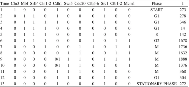
sta-TABLE I: Orbit with initial configuration being the perturbed stationary state. The column “Time” corresponds to the time steps; the columns identified by the nodes correspond to the time evolution of this nodes; the column “Phase” corresponds to the cell cycle phases; the column “I” correspond to the integer notation for the vector states. For Cdh1 in times 8 and 9 the notation 0/1 means that the left state corresponds to Pathhomogand the right one toPathf req.
Time Cln3 Mbf SBF Cln1-2 Cdh1 Swi5 Cdc20 Clb5-6 Sic1 Clb1-2 Mcm1 Phase I
1 1 0 0 0 1 0 0 0 1 0 0 START 273
2 0 1 1 0 1 0 0 0 1 0 0 G1 278
3 0 1 1 1 1 0 0 0 1 0 0 G1 346
4 0 1 1 1 0 0 0 0 0 0 0 G1 14
5 0 1 1 1 0 0 0 1 0 0 0 S 142
6 0 1 1 1 0 0 0 1 0 1 1 G2 1678
7 0 0 0 1 0 0 1 1 0 1 1 M 1736
8 0 0 0 0 0 1 1 0 0 1 1 M 1632
9 0 0 0 0 0/1 1 1 0 1 1 1 M 1888
10 0 0 0 0 0/1 1 1 0 1 0 1 M 1376
11 0 0 0 0 1 1 1 0 1 0 0 M 368
12 0 0 0 0 1 1 0 0 1 0 0 G1 304
13 0 0 0 0 1 0 0 0 1 0 0 STATIONARY PHASE 272
tionary G1 state (272) with the Cln3 activation. Then we de-termine the pathway and its time step. In 106 samples we find 336 different pathways. The pathwayPathf req = [273,
278, 286, 14, 142, 1678, 1736, 1632, 1904, 1392, 368, 304, 272] with 12 time steps is the most frequent. It appears in 10.9% of the minimal interaction set, while the pathway of the Li et al. model appears only in 3.6% of the cases. If we evaluate the average basin size of theG1 fixed point in the ensemble of the cases having the most frequent pathway, we find thatBSf req(272) =1866.7. Note that this average value
is large than BShomog(272) =1764. The only difference
be-tweenPathf reqandPathhomogis that in the phase M the cyclin
complex Cdh1 is turned on at time step 9 inPathf req instead
of time step 11 inPathhomog, as it is shown in table I. Is this
difference meaningful?
The exit of phase M is controlled by the complex APC, which is activated mainly by Cdc20 and Cdh1. The protein Cdc20 actives APC that begins the degradation of Clb2 dur-ing the transition metaphase-anaphase. The second phase of the Clb2 degradation occurs by the linking of Cdh1 with APC, during the telophase. Therefore, the Clb2 degradation needs a sequential action [14]: (i) Cdc20 activating APC and (ii) Cdh1 linking to APC. Although the degradation by APC-Cdc20 is enough to the exit of phase M, the degradation by APC-Cdh1 is essential to keep the G1 phase stable [15]. In the homoge-neous model Cdh1 is turned on simultahomoge-neously with the turn-ing off of Clb2, implyturn-ing that the second degradation mecha-nism is absent. On the other hand, this second mechamecha-nism is present inPathf reqbecause Cdh1 and Clb2 are both turned on
for two time steps. We can conclude that the early activation of Cdh1 is more coherent with the Clb2 degradation mecha-nism.
This results show that not just the big basin of attraction of the stationary state is indeed robust against changes in the coefficients, but with inhomogeneities this basin of attraction gets bigger: 65,5% of the interaction’s minimal set have basin size bigger than 1764, with a maximum value of 1999.
4. CONCLUSIONS
We found that the big basin of attraction is indeed robust against change in the parameterKi,j: 65,3% of the minimal
interaction set haveBS(272)>1764 and the maximum size being 1999. Considering the orbit of the perturbed station-ary state 273 we found that the most frequent orbit (Pf req) is
not the one exhibited by the homogeneous model: the orbit Pf req appears in 10,9% of the minimum coefficient set while
Phomogappears only in 3,6%, that is, this orbit is more robust
against changes on the coefficients. Besides that, the subset of the dynamical systems exhibitingPf reqhas a mean basin size
BSf req=1866,7 that is bigger thanBShomog=1764. Not just
more robust, butPf req has a better biological significance as
we have shown by means of the earlier activation of Cdc1.
Acknowledgments
The authors thank Alcides Castro e Silva for a careful read-ing of the manuscript. JKLS thanks to CNPq and FAPEMIG, Brazilian agencies. LW acknowledges CNPq for financial support.
[1] B. Alberts, D. Bray, J. Lewis, M. Raff, K. Roberts, and J. D. Watson,Molecular Biology of the cell,3rd ed., New York: Gar-land Publishing (1994).
[2] K. C. Chen, A. Csikasz-Nagy, B. Gyorffy, J. Val, B. Novak, and J. Tyson, Mol. Biol.11, 369 (2000).
[3] F. Li, T. Long, Y. Lu, Q. Ouyang, and C. Tang, Proc. Natl. Acad. Sci USA101, 4781 (2004).
[4] F. R. Cross, V. Archambault, M. Miller, and M. Klovstad, Mol. Biol. Cell13, 52 (2002).
[5] K. C. Chen, H. C. Lee, T. Y. Lin, W. H. Li, and B. S. Chen, Bioinformatics20, 1914 (2004).
[6] K. C. Chen, A. Calzone, Csikasz-Nagy, F. R. Cross, B. Novak, and J. J. Tyson, Mol. Biol. Cell15, 3841 (2004).
[7] F. R. Cross, L. Schroeder, M. Kruse, and K. C. Chen, Mol.
Biol. Cell16, 2129 (2005).
[8] B. Futcher, Curr. Opin. Cell Biol.14, 676 (2002). [9] A. W. Murray, Cell116, 221 (2004).
[10] N. T. Ingolia, and A. W. Murray, Curr. Opin. Cell Biol.14, R771 (2004).
[11] M. Tyers, Curr. Opin. Cell Biol.16, 602 (2004).
[12] Y. Zhang, M. Qian, Q. Ouyang, M. Deng, F. Li, and C. Tang, Physica D219, 35 (2006).
[13] G. Stoll, J. Rougemont, and F. Naef, Bioinformatics22, 2539 (2006).
[14] F. M. Yeong, H. H. Lima, C. G. Padmashree, and U. Surana, Mol. Cell 5, 501 (2000).
![FIG. 1: The yeast cell cycle regulatory network [3]. The nodes are identified by the proteins or complex proteins and by the number used in the definition of the dynamical system](https://thumb-eu.123doks.com/thumbv2/123dok_br/18982985.457742/2.892.161.762.76.505/regulatory-network-identified-proteins-complex-proteins-definition-dynamical.webp)