FACULDADE DE ECONOMIA, ADMINISTRAÇÃO E CONTABILIDADE DEPARTAMENTO DE ECONOMIA
PROGRAMA DE PÓS-GRADUAÇÃO EM ECONOMIA
Risk premia estimation in Brazil:
wait until 2041
Elias Cavalcante Filho
Orientador: Prof. Dr. Bruno Cara Giovannetti
São Paulo - Brasil
2016
Prof. Dr. Marco Antonio Zago Reitor da Universidade de São Paulo
Prof. Dr. Adalberto Américo Fischmann
Diretor da Faculdade de Economia, Administração e Contabilidade
Prof. Dr. Hélio Nogueira da Cruz Chefe do Departamento de Economia
Prof. Dr. Márcio Issao Nakane
Risk premia estimation in Brazil:
wait until 2041
Dissertação apresentada ao Programa de Pós-Graduação em Economia do Depar-tamento de Economia da Faculdade de Economia, Administração e Contabilidade da Universidade de São Paulo como requisito parcial para a obtenção do título de Mestre em Ciências.
Orientador: Prof. Dr. Bruno Cara Giovannetti
Versão Corrigida
( ersão original disponível na Faculdade de Economia, Administração e Contabilidade)V
São Paulo - Brasil 2016
Estimação de prêmios de risco no Brasil
:
FICHA CATALOGRÁFICA
Elaborada pela Seção de Processamento Técnico do SBD/FEA/USP
Cavalcante Filho, Elias
Risk premia estimation in Brazil: wait until 2041 / Elias Cavalcante Filho. –
...São Paulo, 2016. 42 p.
Dissertação (Mestrado) – Universidade de São Paulo, 2016. Orientador: Bruno Cara Giovannetti.
1.Risco 2. Prêmios de risco 3. Precificação de ativos 4. Modelos multifatoriais I. Universidade de São Paulo. Faculdade de Economia, Administração e Contabilidade. II. Título.
Agradeço
ao meu orientador Bruno Cara Giovannetti pela orientação e cada ensinamento ao
longo desse trabalho.
aos professores Fernando Chague e Rodrigo De Losso pelas diversas contribuições.
aos meus pais, Elias e Miriam, pela sabedoria compartilhada e aos meus irmãos,
Laura e Alfredo, por todo apoio.
aos meus amigos Eduardo Astorino, Bruno Palialol e Joelson Sampaio pelos vários
conselhos.
Os resultados das estimações de prêmios de risco brasileiros não são robustos na literatura.
Por exemplo, dentre 133 estimativas de prêmio de risco de mercado documentadas, 41 são
positivas, 18 negativas e o restante não é signiĄcante. No presente trabalho, investigamos
os motivos da falta de consenso. Primeiramente, analisamos a sensibilidade da estimação
dos prêmios de risco norte-americanos a duas restrições presentes no mercado brasileiro: o
baixo número de ativos (137 ações elegíveis) e a pequena quantidade de meses disponíveis
para estimação (14 anos). Concluímos que a segunda restrição, T pequeno, tem maior
impacto sobre os resultados. Em seguida, avaliamos as duas potenciais causas de problemas
para a estimação de prêmios de risco em amostras com T pequeno: i) viés de pequenas
amostras nas estimativas dos betas; e ii) divergência entre prêmio de riscoex-post eex-ante.
Através de exercícios de Monte Carlo, concluímos que para o T disponível no Brasil, a
estimativa dos betas já não é mais um problema. No entanto, ainda precisamos esperar até
2041 para conseguirmos estimar corretamente os prêmios ex-ante com os dados brasileiros.
Abstract
The estimation results in the literature on Brazilian risk premia are not robust. For
instance, among the 133 market risk premium estimates reported in the literature, 41
are positive, 18 are negative, and the remainder are not signiĄcant. In this study, we
investigate the grounds for this lack of consensus. First, we analyze the sensitivity of the
US risk premia estimation to two relevant constraints present in the Brazilian market: the
small number of assets (137 eligible stocks) and the short time-series sample available for
estimation (14 years). We conclude that the second constraint, small T, has greater impact
on the results. Then, we evaluate the two potential causes of problems in risk premia
estimations with smallT: i) small sample bias on betas, and ii) divergence betweenex-post
and ex-ante risk premia. Through Monte Carlo simulations, we conclude that for the T
available for Brazil, the beta estimates are no longer a problem. However, it is necessary
to wait until 2041 to be able to estimate ex-ante risk premia with Brazilian data.
1 Introduction . . . . 9
2 Data . . . 13
3 Methodology of risk premium estimation . . . 17
3.1 Multi-factor model . . . 17
3.2 Risk premium estimation . . . 17
4 Risk premium analysis . . . 19
4.1 Full samples analysis . . . 19
4.2 Does the size of N restrict the estimation? . . . 21
4.3 Does the size of T restrict the estimation? . . . 23
4.4 Why is the impact of T so high? . . . 28
5 Conclusion . . . 33
Referências . . . 35
A Appendix . . . 37
A.1 Diferent weights for Brazilian portfolios . . . 37
1 Introduction
The estimation results of Brazilian risk premia show no consensus in the literature.
Reported estimates not only disagree with the US and international results but also vary
among themselves. The Brazilian risk premia estimates collected from several studies1 and
presented in Figure 1 illustrate lack of consensus.
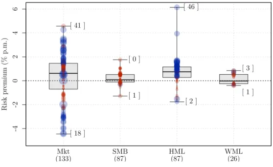
Figure 1 – Dispersion in the risk premia estimations for Brazil
The figure shows the dispersions in the estimations of market (Mkt), size (SMB), value (HML), and momentum (WML) risk premia in the Brazilian stock market. The figure shows a box-plot for each risk factor, and each circle represents one reported estimation (% p.m.). The box-plot reports the 0th, 25th, 50th, 75th, and 100th percentiles. The numbers within the brackets to the right of the 0th and 100th percentiles are the number of negative and positive estimates of each factor respectively. The higher the t-value reported, the larger the circle. A significant estimate (|t-value| ≥ 1.64) is indicated by a blue circle. The coordinate axis reports the factor’s name followed by the number of estimates reported.
-4 -2 0 2 4 6 Risk premium (% p.m.) Mkt
(133) SMB(87) HML(87) WML(26)
[ 41 ]
[ 0 ]
[ 46 ]
[ 3 ]
[ 18 ]
[ 1 ]
[ 2 ]
[ 1 ]
The estimates in Figure 1 are obtained by exploring many sub-periods between
1976 and 2015 and by applying a variety of techniques2. The estimates of the market
(Mkt) risk premium are positive in 41 cases, negative in 18 cases, and not signiĄcant in 74
cases. The size (SMB) of the risk premium does not present any positive and statistically
1
Fama and French (1998), Rouwenhorst (1999), Bonomo and Garcia (2001), Bonomo, Pereira and Schor (2002), Sampaio (2002), Malaga and Securato (2004), Matos (2006), Chague and Bueno (2007), Bellizia (2009), Mussa, Rogers and Securato (2009), Brito and Murakoshi (2009), Mussa et al. (2011), Bodur (2011), Rizzi (2012), Mussa, Fama and Santos (2012), Varga and Brito (2015), Eid Jr and Martins (2015), and Piccoli et al. (2015).
2
10
signiĄcant estimates. The value (HML) risk premium presents the most robust estimates.
Of the 87 estimates, 46 are positive and signiĄcant, and only 2 are signiĄcant and negative.
Finally, there are 26 estimates for the momentum (WML) risk premium, but only a few
cases are signiĄcant, with three positives and one negative.
This paper investigates the reasons behind the lack of robustness in the estimations
of Brazilian risk premia. First, we analyze the sensitivity of the US risk premia estimations
to two relevant constraints present in the Brazilian market: the small number of assets
(small �) and the short time-series samples (small�).3
We conclude that the restriction imposed by the small T is more relevant than
that imposed by the small N. While Brazilian data ofer values of T over 14 years, our
analysis indicates that it is necessary to analyze a time-series sample using data exceeding
40 years to obtain robust risk premia estimates. On the other hand, the Brazilian value of
N does not pose an issue.
Given these results, we then investigate the problems caused by the smallT. One
problem could be the use of poorly estimated betas in the second stage of the estimation.
Another problem could be the use of poorly estimated expected returns of stocks. Both
would induce errors in the estimation of the risk premia. Poorly estimated betas generate
biased risk premia estimates. Poorly estimated expected returns lead to the estimation of
ex-post instead of ex-ante risk premia.4
To assess the relative importance of these two issues, we perform Monte Carlo
simulations. We conclude that the most important issue is the use of poorly estimated
expected returns. Indeed, the diference between ex-post andex-ante risk premia proves
to be signiĄcant when the estimation is performed with the small T available for Brazil.
For instance, when data are simulated using a market risk premium of 0.65% p.m., we
3
There are few liquid stocks in Brazil. In 2000, only 37 stocks could be considered liquid. In 2014, this number increased to 137. The details on the liquidity criteria can be found at the NEFIN website (<http://nefin.com.br>). Moreover, until 1999, the risk-free rate was used as an instrument of the pegged exchange rate regime, and it was often set to very high levels. Therefore, to estimate the risk premia in Brazil, one commonly uses data beginning in the year 2000.
4
estimate a positive and signiĄcant risk premium in only 17% of the samples.
Our main conclusion is that one needs to wait until 2041 to be able to safely
estimate the ex-ante risk premia for Brazil. Anyone interested in computing the cost of
equity for Brazilian Ąrms should use Brazilian data only to estimate the betas. In turn,
the price of risk should be taken from data with longer time-series sample, US data, for
instance.
The remainder of the paper is organized as follows. Section 2 describes the dataset,
followed by the Ąrst analysis of portfolios and risk factors. Section 3 presents the factor
model we use in the estimation as well as the methodology supporting it. Section 4 compares
the premia results for the US with those found for Brazilian markets (4.1), followed by
the analysis of the impact of estimating risk premia with a small number of assets (4.2)
and with small time-series samples (4.3). This section ends with the assessment of the
consequences of estimating risk premia with small time-series samples (4.4). Section 5
2 Data
The main paperŠs datasets consist of monthly portfolio returns from and risk factors
of the Brazilian and the US stock markets. The US information is obtained from FrenchŠs
website1 and covers the period between January 1927 and December 2014. The Brazilian
information is taken from the Brazilian Financial Studies Lab (NEFIN2) and covers the
period from January 2001 to December 2014. The Brazilian stock market was already
operational prior to this period. However, until 1999, the risk-free rate was used as an
instrument of the pegged exchange rate regime, and it was often set to very high levels.
Therefore, to estimate the risk premia in Brazil, one commonly uses data beginning in
the year 20003. The US portfolio and risk factor returns are value-weighted, while the
Brazilian ones are equally weighted4.
The 22 portfolios used in this work are presented in Table 1. This table is organized
as follows. The Ąrst column shows the variables used to arrange the assets into portfolios.
The second column names each portfolio, the third and fourth columns contain the
percentiles used as breakpoints for the construction of the portfolios, the Ąfth and sixth
columns report the means of the portfoliosŠ returns, and, Ąnally, the last two columns list
the autocorrelation consistent standard deviations. The data available at NEFINŠs and
FrenchŠs websites have diferent numbers of portfolios. Therefore, in order to conduct a
fair comparison between the Brazilian and the US markets, some portfolios are combined
by calculating their value-weighted returns. The Ąrst 17 portfolios are deĄned based on
information about Size, Book-to-market, and Momentum, and the other portfolios are
organized by grouping assets of the same industry. Note that both countries have the same
number of industry portfolios; however, some industries appear only in one of the markets.
Table 1 shows that the US portfoliosŠ returns are negatively correlated with Size and
positively correlated with Book-to-market and Momentum, as described in the literature.
1
<http://mba.tuck.dartmouth.edu/pages/faculty/ken.french/data_library.html>.
2
Núcleo de Pesquisas em Economia Financeira da Universidade de São Paulo
<http://nefin.com.br>.
3
The first year is used to select the eligible assets.
4
14
Table 1 – US and Brazilian portfolios
Portfolios of the the US and Brazilian asset market. The portfolios differ between countries by their breakpoints and the period contemplated. Their means were calculated on the excess of return and the standard deviation are autocorrelation consistent.
Breakpoints Mean (% p.m.) Sd (% p.m.)
Variables Labels
US
Jan/1927 - Dec/2014 (1056 months)
BRA Jan/2001 - Dec/2014
(168 months)
US BR US BR
Size
Small [0,30] [0,33.3] 1.00*** 0.25 8.44 8.01
Medium size [30,70] [33.3,66.6] 0.88*** 0.25 6.78 6.99
Big [70,100] [66.6,100] 0.63*** 0.12 5.25 6.20
Book-to-market
Low [0,10] [0,33.3] 0.58*** 0.10 5.77 6.74
Medium bm [30,70] [33.3,66.6] 0.72*** 0.13 5.78 6.99
High [90,100] [66.6,100] 1.09*** 0.49 9.22 7.17
Momentum
Loser [0,30] [0,33.3] 0.37 -0.42 7.71 8.61
Normal [30,70] [33.3,66.6] 0.63*** 0.44 5.62 6.29
Winner [70,100] [66.6,100] 0.98*** 0.71 5.61 6.36
Size x Book-to-market
Small Low [0,50 ; 0,20] [0,50 ; 0,50] 0.65*** 0.24 8.09 7.70
Small High [0,50 ; 80,100] [0,50 ; 50,100] 1.27*** 0.47 8.77 8.06
Big Low [50,100 ; 0,20] [50,100 ; 0,50] 0.62*** 0.15 5.47 6.21
Big High [50,100 ; 80,100] [50,100 ; 50,100] 0.99*** 0.08 8.12 6.77
Size x Momentum
Small Loser [0,50 ; 0,30] [0,50 ; 0,50] 0.55* -0.14 9.21 8.88
Small Winner [0,50 ; 70,100] [0,50 ; 50,100] 1.35*** 0.84 7.30 7.08
Big Loser [50,100 ; 0,30] [50,100 ; 0,50] 0.38 -0.08 7.63 7.25
Big Winner [50,100 ; 70,100] [50,100 ; 50,100] 0.94*** 0.42 5.56 5.79
Basic Products - Basic Products 0.48 7.83
Consumer Consumer Consumer 0.72*** -0.09 5.35 6.81
Energy - Energy 0.26 7.13
Industry HiTec HiTec - 0.67*** - 5.64
-Healthcare Healthcare - 0.81*** - 5.63
-Manufacturing Manufacturing Manufacturing 0.69*** 0.88 5.59 8.70
Other Other Other + Finance 0.63*** 0.40 6.50 7.39
Significance: * 10%; ** 5%; ***1%.
The Brazilian portfolios also generally exhibit the same behavior as those of the US market.
However, three points require attention: i) the Book-to-market efect is not observable
among the Big High and Big Low portfolios, since Big High presents an average return
of 0.08, which is smaller than the average return of 0.15 for Big Low, ii) the Size efect
is also not observed between the Big Loser and Small Loser portfolios, since the Small
Loser has lower average return, and iii) none of the Brazilian portfoliosŠ returns have a
signiĄcant average.
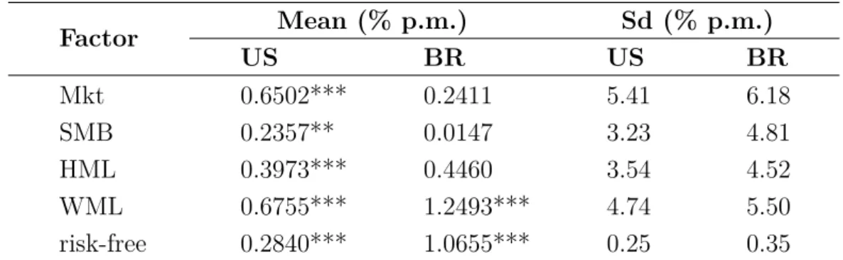
Besides the mentioned portfolios, we use four risk factors and a risk-free rate for
each economy. Table 2 presents the mean and standard deviation of those variables. The
names used for each factor are provided in the Ąrst column. They are Mkt for the Market
Table 2 – Factors and risk-free rate
Factors and risk-free rates of the US and Brazilian markets. The information refers to the period between January 1927 and December 2014 for the American market and between January 2001 and December 2014 for the Brazilian market. The table present the means for each factor and the respective autocorrelation consistent standard deviation.
Factor Mean (% p.m.) Sd (% p.m.)
US BR US BR
Mkt 0.6502*** 0.2411 5.41 6.18
SMB 0.2357** 0.0147 3.23 4.81
HML 0.3973*** 0.4460 3.54 4.52
WML 0.6755*** 1.2493*** 4.74 5.50
risk-free 0.2840*** 1.0655*** 0.25 0.35
Significance: * 10%; ** 5%; ***1%.
risk-free rate used for the US is the Treasury bill month rate, and for the Brazilian market,
we use the 30-day Deposito Interbancário (DI) swap rate.
Again the variables for the US follow the pattern documented in the literature,
that is, all factors have positive and statistically signiĄcant return averages. On the other
hand, the Brazilian data show signiĄcance only for WML, despite the fact that all factors
3 Methodology of risk premium estimation
This section explains how the risk premium is estimated. In order to do so, we Ąrst
present the multi-factor model in subsection 3.1, and then explain the methodology for
the model estimation.
3.1
Multi-factor model
DeĄne � as the number of risk factors, � as the number of assets, and � as the
number of observed periods. The multi-factor model assumes that excess asset returns are
governed by the following linear relation:
�(���) =Ð+Ñ�′Ú (3.1)
where��
� is the excess return of an asset �∈ {1,2, ..., �}, Ð is the model pricing error,Ú
is a �x1 vector with the risk premia for the � factors, and� is a �x1 vector with the
risk measures of asset � for each factor.
The model also proposes that the � vector respect the following relation in the
time series:
����=��+Ñ�′��+��� (3.2)
where��
�� is the excess return of asset� in period�∈ {1,2, ..., �},�� is the expected pricing
error of asset �, �� is a ��1 vector with the realizations of the factors in period �, and ���
is the random error of asset �in period �.
3.2
Risk premium estimation
The model estimation is conducted using the GMM methodology introduced by
Hansen (1982), with a similar framework proposed by Cochrane (2001). This methodology
provides a joint estimation of all parameters of the model and easily handles the problems
18
The GMM estimation is based on the hypotheses derived from the modelŠs
intro-duction in Section 3.1. We can build the following matrix using the modelŠs assumptions:
��(�, Ñ, Ð, Ú) =
︀ ︀ ︀ ︀ ︀ ︀ ︀ ︀ (��
�−�−Ñ��)
[(��
�−�−Ñ��)⊗��]
[1, Ñ′] [(���−Ð−ÑÚ)]
︀ ⎥ ⎥ ⎥ ⎥ ⎥ ⎥ ︀
([�+� �+1+�]x1)
(3.3)
where ��
� is the �x1 vector of excess returns in period �, �� is the �x1 vector of risk
factors in period �, such that�∈ {1,2, ..., �},⊗ is the Kronecker operator, � is the�x1
vector of expected pricing errors for each asset, Ñ is the �x� matrix of risk related to
each asset and factors of the model, Ð is the expected pricing error of the model, Ú is the
Kx1 vector of risk premia for each risk factor, and 1 is a 1xN vector of ones.
From the modelŠs assumptions, we know that the expected value of each line of the
matrix equals zero. The GMM method estimates the parameters (^�,Ñ,^ Ð,^ ^Ú) by solving the
following optimization:
︁ ^
�,Ñ,^ Ð,^ ^Ú︁= argmin
¶�,Ñ,Ð,Ú♢
�
︁
�=1
[��(�, Ñ, Ð, Ú)]′�⊗1 �
︁
�=1
[��(�, Ñ, Ð, Ú)] (3.4)
where� is a weighting matrix of moments, which is typically set to generate as efective
estimates as possible. However, since the number of parameters and equations are the
same, the weighting matrix does not afect the estimation. Thus, we use the identity matrix
to solve the problem.
Finally, we have the following matrix of variance and covariance parameters:
� ��(^�,Ñ,^ Ð,^ Ú^) = (�′� �)⊗1(�′� �� �)(�′� �)⊗1 (3.5)
where�is the derivate of��with respect to the parameter vector (�= �[���/�(�, Ñ, Ð, Ú)]),
� is the identity matrix ([� +� �+ 1 +�]), and � = �(����′) is estimated using the
4 Risk premium analysis
4.1
Full samples analysis
The Brazilian risk premia diagnostic starts by taking the US stock market as the
benchmark and comparing the results between both markets. The Mkt,SMB, HML, and
WML risk premia are estimated using data from January 1927 to December 2014 for the
US stock market, and from January 2001 to December 2014 for the Brazilian one.
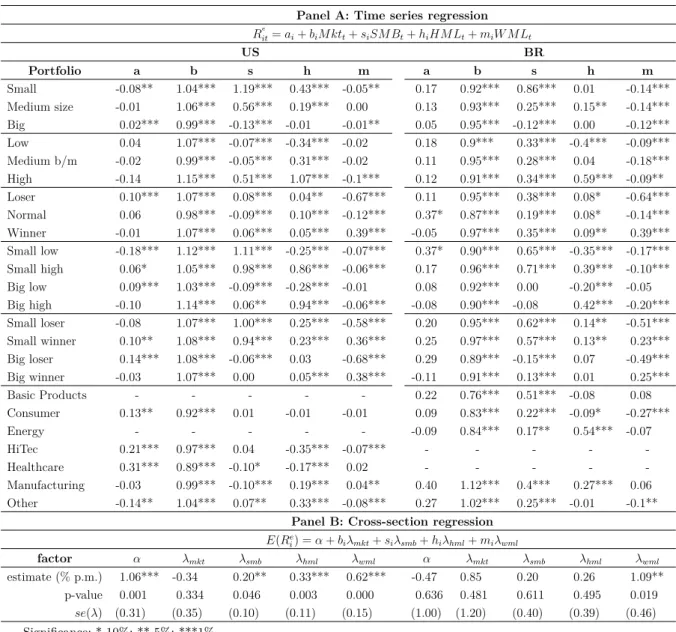
Table 3 presents the results, which are organized in two panels. Panel A presents
the estimated parameters for the time series regression, with the risk measures of each
portfolio. Panel B arranges the cross-section regression results, with the risk premia
estimates followed by their p-values and standard error deviations. In both panels, the
values on the left refer to the US, and on the right, to Brazil.
The results for the time series in Panel A show some similarities between both
markets. As expected, the US market data conĄrm the patterns widely documented
in the literature. Most values of the intercept � are not signiĄcant and, despite some
signiĄcant cases, they do not demonstrate correlation with the variables Size,
Book-to-market, and Momentum. The values of � are mostly around 1.00, with low variation
between portfolios, and the parameters �, ℎ, and � behave according to the ordering
patterns reported for the portfolios returns. In other words, the lower the value of the
assets that integrate the portfolios , the higher the estimated values of�; on the other hand,
ℎand�grow positively correlated with portfolios ordered by the variables Book-to-market
and Momentum, respectively.
In the Brazilian case, most of the patterns observed in the US time-series regression
repeat themselves with a few caveats. First, the estimates of � show a lower frequency of
signiĄcant cases, which goes in favor to the modelŠs adjustment to the data . In addition,
the parametersŠ estimates follow the same order highlighted in the results of the US
data. � is negatively correlated with Size, and ℎ and � are positively correlated with
20
Table 3 – Full sample regression
The table presents the estimated values for the United States (US) and Brazil (BR) of the parameters of the time series regression (equation 3.2) in Panel A and cross-section regression (equation 3.1) in Panel B. The periods used for the estimates cover January 1927 to December 2014 to the United States, and January 2001 to December 2014 for Brazil.
Panel A: Time series regression
�e
��=��+��� ���+���� ��+ℎ��� ��+��� � ��
US BR
Portfolio a b s h m a b s h m
Small -0.08** 1.04*** 1.19*** 0.43*** -0.05** 0.17 0.92*** 0.86*** 0.01 -0.14*** Medium size -0.01 1.06*** 0.56*** 0.19*** 0.00 0.13 0.93*** 0.25*** 0.15** -0.14*** Big 0.02*** 0.99*** -0.13*** -0.01 -0.01** 0.05 0.95*** -0.12*** 0.00 -0.12*** Low 0.04 1.07*** -0.07*** -0.34*** -0.02 0.18 0.9*** 0.33*** -0.4*** -0.09*** Medium b/m -0.02 0.99*** -0.05*** 0.31*** -0.02 0.11 0.95*** 0.28*** 0.04 -0.18*** High -0.14 1.15*** 0.51*** 1.07*** -0.1*** 0.12 0.91*** 0.34*** 0.59*** -0.09** Loser 0.10*** 1.07*** 0.08*** 0.04** -0.67*** 0.11 0.95*** 0.38*** 0.08* -0.64*** Normal 0.06 0.98*** -0.09*** 0.10*** -0.12*** 0.37* 0.87*** 0.19*** 0.08* -0.14*** Winner -0.01 1.07*** 0.06*** 0.05*** 0.39*** -0.05 0.97*** 0.35*** 0.09** 0.39*** Small low -0.18*** 1.12*** 1.11*** -0.25*** -0.07*** 0.37* 0.90*** 0.65*** -0.35*** -0.17*** Small high 0.06* 1.05*** 0.98*** 0.86*** -0.06*** 0.17 0.96*** 0.71*** 0.39*** -0.10*** Big low 0.09*** 1.03*** -0.09*** -0.28*** -0.01 0.08 0.92*** 0.00 -0.20*** -0.05 Big high -0.10 1.14*** 0.06** 0.94*** -0.06*** -0.08 0.90*** -0.08 0.42*** -0.20*** Small loser -0.08 1.07*** 1.00*** 0.25*** -0.58*** 0.20 0.95*** 0.62*** 0.14** -0.51*** Small winner 0.10** 1.08*** 0.94*** 0.23*** 0.36*** 0.25 0.97*** 0.57*** 0.13** 0.23*** Big loser 0.14*** 1.08*** -0.06*** 0.03 -0.68*** 0.29 0.89*** -0.15*** 0.07 -0.49*** Big winner -0.03 1.07*** 0.00 0.05*** 0.38*** -0.11 0.91*** 0.13*** 0.01 0.25***
Basic Products - - - 0.22 0.76*** 0.51*** -0.08 0.08
Consumer 0.13** 0.92*** 0.01 -0.01 -0.01 0.09 0.83*** 0.22*** -0.09* -0.27***
Energy - - - -0.09 0.84*** 0.17** 0.54*** -0.07
HiTec 0.21*** 0.97*** 0.04 -0.35*** -0.07*** - - - -
-Healthcare 0.31*** 0.89*** -0.10* -0.17*** 0.02 - - - -
-Manufacturing -0.03 0.99*** -0.10*** 0.19*** 0.04** 0.40 1.12*** 0.4*** 0.27*** 0.06 Other -0.14** 1.04*** 0.07** 0.33*** -0.08*** 0.27 1.02*** 0.25*** -0.01 -0.1**
Panel B: Cross-section regression
�(��
�) =Ð+��Ú���+��Ú���+ℎ�Úℎ��+��Ú���
factor Ð Ú��� Ú��� Úℎ�� Ú��� Ð Ú��� Ú��� Úℎ�� Ú���
estimate (% p.m.) 1.06*** -0.34 0.20** 0.33*** 0.62*** -0.47 0.85 0.20 0.26 1.09** p-value 0.001 0.334 0.046 0.003 0.000 0.636 0.481 0.611 0.495 0.019
��(Ú) (0.31) (0.35) (0.10) (0.11) (0.15) (1.00) (1.20) (0.40) (0.39) (0.46)
Significance: * 10%; ** 5%; ***1%.
estimates than those observed for the US market.
In contrast, the cross-section results in Panel B indicate some divergence between
BrazilŠs and the USŠ risk premia estimations. The results for the US demonstrate signiĄcant
risk premia for all factors except the market factor, which supports the capacity of the
model to Ąt the US data. On the other hand, the Brazilian results reject the modelŠs ability
to replicate the returns of assets, since only the factor WML demonstrates a positive and
The analysis of this result by itself could lead to the precipitated conclusion that the
multi-factor model does not Ąt Brazilian data. However, this result should be interpreted
with caution. Therefore, in order to identify the source of the problem, we conduct a more
careful analysis of two points that distinguish both markets: i) the size of �, that is, the
number of assets used to build the portfolios in the estimation process, and ii) the size of
�, that is, the length of the time-series sample of the Brazilian data. The next step is to
investigate the impact of these divergences.
4.2
Does the size of
N
restrict the estimation?
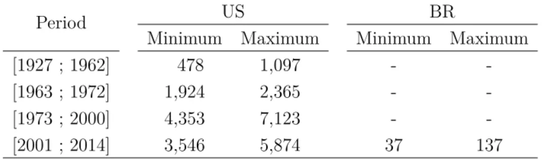
There is a huge diference between the number of assets available in the US and
Brazilian markets. Table 4 reports the number of eligible assets1 for both markets and
organizes this information in sub-periods2.
Table 4 – Number of eligible assets
The table indicates the maximum and minimum number of eligible assets observed for each sub-period and stock market.
Period US BR
Minimum Maximum Minimum Maximum
[1927 ; 1962] 478 1,097 -
-[1963 ; 1972] 1,924 2,365 -
-[1973 ; 2000] 4,353 7,123 -
-[2001 ; 2014] 3,546 5,874 37 137
While the number of US assets varies, ranging from 478 to 7,123 in a history of 84
years, we observe a maximum of 137 assets over the 14-year period analyzed for Brazil.
This result may be attributed to the portfolio behavior, since the fewer the assets used to
build a portfolio, the greater the idiosyncratic risk impact on the portfolioŠs returns.
1
In both markets, some eligibility rules are applied to select the assets that compose the portfolios. The US’ and Brazil’s rules are listed at French’s website and NEFIN’s website respectively.
2
22
The small number of assets could afect the risk premium estimation in two ways:
i) by generating distortion in the portfoliosŠ returns, which are used as dependent variables
in the regressions, and ii) by impacting the estimations of the risk factors. The Ąrst concern
is discarded by analyzing the standard deviations of the returns on the 22 portfolios for
both markets, reported in Table 1. One can see that the standard deviations are quite
similar between the markets, and there is no pattern. This means that the standard
deviations of the Brazilian data are not always greater than those of the US data. This
indicates that no relevant distortions are generated in the Brazilian portfolios, which are
used as dependent variables. However, the second highlighted concern demands more
attention, considering that, as reported in Table 2, all the risk factors in the Brazilian case
show higher standard deviations than those of the US.
The procedure to calculate the risk factors is based on building portfolios using the
correlated assetsŠ characteristics with the returns and then deĄning the returns on those
portfolios as realizations of the risk factors (FAMA; FRENCH, 1993; CARHART, 1997).
For example, the factor realization SMB is obtained by calculating the return from a
portfolio long in small assets and short in big assets. However, considering the low number
of assets available in Brazil, risk factor estimation by this procedure can be afected by
the assetŠs idiosyncratic risk. This could explain the pattern observed with regard to the
standard deviation of Brazilian factors in Table 2, or the results observed for the risk
premia estimations in Panel B of Table 3, in which most parameters have non-signiĄcant
estimates.
In order to measure the impact of this feature on risk premia estimation, we decrease
the number of assets used in the estimation of the US risk factors to a similar number of
assets available for the Brazilian market and verify if the risk premia signiĄcance frequency
is afected. Therefore, we run the following procedure 1,000 times: i) for each year of the 84
years of historical data, we select a sample of 37 or 137 assets, and use them to estimate
the risk factor realization for the months of the respective year, and ii) we process the risk
premia estimation and verify if the estimated Ú�, such that � ∈ {���, ���, ℎ��, ���},
Two methods of sample selection are applied. The Ąrst one, denominated ŞRandom,Ť
is a random selection from the eligible assets of each year of the 84 yearsŠ samples. The
second, denominated ŞSize x Book-to-marketŤ, intends to preserve the distribution on the
variables Size and Book-to-market among the selected assets3.
The results obtained from this procedure are presented in Table 5. The Ąrst column
reports the selection method applied, the second indicates the number of assets selected
each year, and the remaining columns show the percentages from the 1,000 estimations that
return positive and signiĄcant estimates of the parameters Ð,Ú���, Ú���,Úℎ��, and Ú���.
We run both selection methods with 37 and 137 assets, the two extreme cases observed in
the Brazilian data. The results using 37 assets are presented in Figure 2, where we plot
the observed density of the t-values estimated for each risk factor.
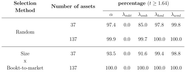
The results show that most of the parameters are barely afected. The most afected
parameter is the SMB risk premium, which has around 85% to 92% of signiĄcant estimates
when 37 assets are used to build the risk factors, but this result changes to around 99%
when 137 assets are used. The second most afected risk premium is HML, and its biggest
impact is observed with the random selection with 37 assets; 97.8% of the estimates are
signiĄcant. WML has a very small impact and shows more than 98% signiĄcant estimates
in all cases. Mkt shows non-signiĄcant results in all cases. Finally, the mean pricing error
(Ð) has more than 93% of signiĄcant and positive estimates.
The results show that most of the risk factors calculated using 37 or more assets
reach the same outcome as when the whole set of assets is used. In other words, there is no
indication that the number of assets available for the risk premium estimation generates a
big impact in the Brazilian case.
4.3
Does the size of
T
restrict the estimation?
While the US risk premia results are based on 84 years of historical data, the
Brazilian market, for which we conduct the regression, has only 14 years of data. In order
3
24
Table 5 – Percentage of significant cases by the number of assets
Selection
Method Number of assets
percentage (�≥1.64)
Ð Ú��� Ú��� Úℎ�� Ú���
Random
37 97.4 0.0 85.0 97.8 99.8
137 99.9 0.0 99.7 100.0 100.0
Size x
Bookt-to-market
37 93.5 0.0 91.6 99.4 98.8
137 100.0 0.0 100.0 100.0 100.0
Figure 2 – Density of �Úˆ estimated with factors for 37 assets
Ð
0.5
1.5 Method
Random
Size x Book-to-market
Mkt
0.5 1.5
SMB
0.5 1.5
HML
0.5 1.5
WML
0.5 1.5
-1.64 0 1.64
to verify whether this divergence is a constraint for Brazilian risk premia estimations, we
risk premia estimations.
The analysis uses the US risk factors and portfoliosŠ returns presented in Section 2,
and the procedure is described as follows: i) to deĄne a time window length that has
the same number of months as the Brazilian data (168 months), ii) to estimate as many
regressions as possible on the US data using only the number of months deĄned in the
previous step, that is, starting with the oldest 168-month window allowed until the most
recent one, and always dropping the oldest month in exchange for a more recent one. The
results are the risk premia estimates for December 1940 to December 2014, using the data
of only the last 168 months available. At the end of this procedure, we have a total of 889
sets of estimates.
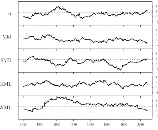
Based on the results obtained from the described procedure, we draw Figure 3.
Each graphic in the Ągure is related to one parameter, Ð, Ú���,Ú���, Úℎ��, or Ú���, and
each point of each graphic indicates the t-value obtained for a particular parameter from
an estimated model with the last 168 months observed at the reference date. Therefore,
Figure 3 is nothing but a history of 889 t-values for each risk premium estimated with the
US data, using Ąxed windows of 168 months. In addition, each graph is accompanied by a
dotted line at value 1.64, which is the critical value adopted for rejecting the hypothesis
that the parameter is less than or equal to zero.
The results indicate the importance of time-series sample size for the factor model
estimation and demonstrate that, even with the US data, it is not uncommon to Ąnd that
risk premia are not signiĄcant when short time-series samples are used. It is also notable
that WML is the most robust factor, just as in the Brazilian case. At the start of the
analysis of the market risk premium, we observe that, in most estimates, this parameter is
not signiĄcant, except for a few points at the beginning of the historical data. SMB risk
premium shows signiĄcance only in a few periods, mostly at the beginning of the historical
data, but we can Ąnd some signiĄcant points in the middle and in very recent periods.
The parameters relate to HML and WML, which, on the other hand, are more robust,
26
Figure 3 – History of t-values for an estimation window of 14 years
Each point in the figure is the t-value of the parameterÐ,Ú���,Ú���, Úℎ��, orÚ��� resulting
from the estimation of a model with all the factors and 168 months (14 years) of data. The horizontal dotted line crosses the ordinate axis at 1.64, the critical value to reject the hypothesis that the estimated values are equal to or smaller than zero, with a significance level of 5%.
Ð -2 0 2 4 Mkt -2 0 2 4 SMB -2 0 2 4 HML -2 0 2 4 WML -2 0 2 4
1940 1950 1960 1970 1980 1990 2000 2010
true for the second factor, which is signiĄcant for almost the entire history.
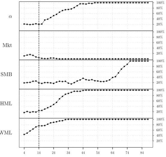
After establishing the importance of time-series sample size to risk premia
esti-mation, we verify how sensitive the estimation is to the time-series sample size. To do
so, we apply the following procedure: i) we select several window lengths (48, 72,..., 1056
months), ii) for each option selected in the previous step, we repeat the procedure applied
to build Figure 3 and compute the percentage that each risk premium is signiĄcant. This
analysis is presented in Figure 4. The Ąve graphs in the Ągure indicate the signiĄcance of
each parameter according to the window used for the estimations. The dotted line crossing
the graphics vertically highlights the percentage obtained with windows of 14 years, the
Figure 4 – Percentage of significant cases by the number of years
The graph below shows the percentages for which the t-values of the parametersÐ,Ú���,
Ú���, Úℎ��, andÚ��� are greater than 1.64, according to the time-series sample size used for
the estimations. The dotted line crossing the graphics vertically highlights the percentage obtained with windows of 14 years.
Ð 20% 40% 60% 80% 100% Mkt 20% 40% 60% 80% 100% SMB 20% 40% 60% 80% 100% HML 20% 40% 60% 80% 100% WML 20% 40% 60% 80% 100%
4 14 24 34 44 54 64 74 84
Number of years used for estimation
The results indicate that a large time-series sample is required in order to obtain
robust estimates. We start with the parameter Ð, which shows positive and signiĄcant
results around 20% of the time when 14 years are used for the estimation. However, as the
time-series sample becomes larger, it becomes increasingly evident that the data do not
support the zero mean error hypothesis. The market risk premium, on the other hand,
demonstrates robust results independent of the time-series sample length. Most results for
this parameter do not demonstrate positive and signiĄcant estimates. The results of the
28
than 40% of the estimates are positive and signiĄcant even with 64 years. The other two
parameters again demonstrate themselves as more robust. Their estimations seem to be
less sensitive to window size. HML risk premium has about 20% signiĄcant estimations
when 14 years are used, and this percentage reaches 80% with 30 years. TheWML factor
seems to be the most robust of all. Its results are positive and signiĄcant about 80% of
the time when 14 years or more are used for the estimation.
This section demonstrates that the time-series sample size is a relevant restriction
on Brazilian risk premia estimation. Based on the US data, we demonstrate how common
it is to estimate non-signiĄcant risk premia when the number of observed periods is too
short. Furthermore, it seems that one should not expect robust results on factor models to
which time-series samples shorter than 40 years are applied.
4.4
Why is the impact of
T
so high?
The analysis of Brazilian risk premia shows that most of the parameters have
non-signiĄcant estimates. In addition, we demonstrate that the source of the problem is
not the small number of assets available or their characteristics, but the short historical
data of the Brazilian market. The next step is to understand why the Şsize of TŤ has such
a considerable impact and the consequences of applying a factor model to such a short
time-series sample.
The literature on risk premiums estimated with a small T began with Shanken
(1992), followed by Jegadeesh and Noh (2013), Kim and Skoulakis (2014), Raponi, Robotti
and Zafaroni (2015), and Bai and Zhou (2015). Two points emerge from an analysis of
risk premium estimations with a small time-series sample: i) small sample bias on betas,
and ii) divergence between ex-post and ex-ante risk premia.
To understand these consequences, note that as presented in Equation 3.1, the
and risk compensation (Ñ′
�Ú). However, the relation used in the risk premia estimation is
¯
��� =Ð*+ ^Ñ�′Ú* (4.1)
where ¯��
� is the average excess return from asset�, ^� is the estimated risk vector from asset
�, and Ð* andÚ* are the parameters resulting from this relation. Thus, while Equation 3.1
has only true parameters, Equation 4.1 consists only of estimated values.
The Ąrst divergence arises from using the estimated beta ( ^Ñ�) instead of the true
beta (�). According to Shanken (1992), since the independent variable in Equation 4.1 is
measured with error, the estimator is subject to an errors-in-variables problem, making it
biased in small samples. However, the measurement error declines as � increases. Hence,
Shanken (1992) shows how the asymptotic standard errors are inĆuenced by the estimation
error in the betas and proposes an adjustment for the standard errors and a bias-adjusted
estimator. Simulating studies with the US data show a bias of about −16% and −20%
when less than 172 months are used in the risk premium estimation (RAPONI; ROBOTTI;
ZAFFARONI, 2015; BAI; ZHOU, 2015; JEGADEESH; NOH, 2013).
The second divergence is caused by the use of the average excess return instead
of its true expected value. Averaging (3.2) over time, imposing (3.1), and noting that
�(��
�) = ��+Ñ�′�(�) yields
¯
�=Ð+Ñ︁Ú−�(�) + ¯�︁
. (4.2)
Equation 4.2 demonstrates that the relation between the true beta and the average
excess return results in the so-called ex-post risk premium, Ú� =Ú−�(�) + ¯�, which is
equal to the sum of the ex-ante risk premium and the unexpected factor outcomes. Since
one cannot hope for ¯� to be a good estimation of�(�) unless� is large, as Shanken (1992)
points out, it is not possible to obtain a consistent estimate of Ú when � is Ąxed.
30
premia estimation, we perform a Monte Carlo simulation based on the following set-up:
�� =Ú+�� (4.3)
�� =��+�� (4.4)
such that � ∈ {1,2, ..., �}, �� ∼ �(0, à2), �� ∼ �(0,Σ), and �� ⊥ ��. Ú = 0.6502 and
à = 5.41, which are the mean and standard deviation respectively with regard to the US
market risk factors in Table 2. Ñ is the 1�22 vector of the market risk measure from the
US market, whose values are presented in Panel A (see the Ąrst column) of Table 3. Σ
is the 22�22 residual covariance matrix resulting from the US time-series regression in
Section 4.1.
Based on this set-up, we select several values of�, and for each of them, we simulate
10,000 draws. We then estimate the risk premium of each draw by two methods: i) the
same method presented in Section 3.2 and applied to our paper so far, and ii) a modiĄed
estimation in which the risk premium is estimated using the true betas instead of the
estimated values. The simulation allows the analysis of several time-series sample sizes,
and we can isolate the ex-post impact using the true betas in the estimation procedure.
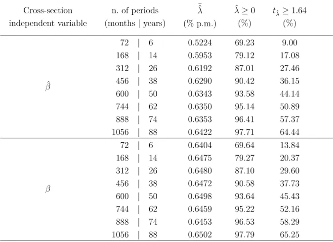
Table 6 presents the results obtained for the risk premium estimation using the
estimated beta or the true beta, both for several values of T, varying from 72 to 1056
months. The Ąrst column indicates the risk measure used as the independent variable, the
true beta ( ^Ñ) or the estimated beta (Ñ). The second column shows the number of months
used (T), the third column reports the means of the estimated risk premiums, the fourth
column reports the percentage of the 10,000 simulations with a positive estimated value,
and the Ąfth column shows the percentage of positive and signiĄcant estimates.
The results conĄrm that, as expected, the risk premium obtained with the estimated
beta is in fact biased, as demonstrated by Raponi, Robotti and Zafaroni (2015), Bai and
Zhou (2015), Jegadeesh and Noh (2013). When the time-series sample has only 72 or 168
months of data, estimates are biased by about -20% and -8% respectively , and for the
estimations with 1056 months, the bias is around 1%. In contrast, the estimation provided
Table 6 – Simulation results
The table presents the results obtained for the risk premium estimation using the estimated beta or the true beta for time-series samples varying from 72 to 1056 months. The first column shows which risk measure was used as the dependent variable, the true beta ( ˆÑ) or the estimated beta (Ñ). The second column shows the number of months used. The third column reports the means of the estimated risk premiums. The fourth column indicates the percentage the 10,000 simulations with a positive estimated value, and the fifth column reports the percentage of positive and significant estimates.
Cross-section independent variable
n. of periods (months | years)
¯^
Ú
(% p.m.) ^
Ú≥0
(%)
�ˆÚ ≥1.64
(%)
^
Ñ
72 | 6 0.5224 69.23 9.00
168 | 14 0.5953 79.12 17.08
312 | 26 0.6192 87.01 27.46
456 | 38 0.6290 90.42 36.15
600 | 50 0.6343 93.58 44.14
744 | 62 0.6350 95.14 50.89
888 | 74 0.6353 96.41 57.37
1056 | 88 0.6422 97.71 64.44
Ñ
72 | 6 0.6404 69.64 13.84
168 | 14 0.6475 79.27 20.37
312 | 26 0.6480 87.10 29.60
456 | 38 0.6472 90.58 37.73
600 | 50 0.6498 93.64 45.43
744 | 62 0.6459 95.22 52.16
888 | 74 0.6453 96.53 58.29
1056 | 88 0.6502 97.79 65.25
However, the percentage of positive and signiĄcant estimates is almost the same
irrespective of the beta used. The percentage of positive and signiĄcant estimates is between
9% and 14% for the 72-month time-series sample, about 17% to 20% for the time-series
samples of 168 months, and about 64% to 65% for 1056 months.
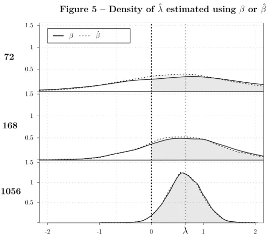
The same conclusion can be drawn from the analysis of Figure 5. This Ągure shows
three graphics, one for each option of time-series sample length (72, 168, or 1056 months).
Each graph has two density curves for the estimated risk premium, one derived from the
estimations using the true beta, and the other from those using the estimated beta.
32
Figure 5 – Density of Ú^ estimated using Ñ or Ñ^
0.5 1 1.5
72
Ñ Ñ^
0.5 1 1.5
168
-2 -1 0 1 2
0.5 1 1.5
1056
Ú
results obtained from estimations with the true beta or the estimated beta, and show
that relevant changes only occur by the addition of more months to the estimation. These
results indicate that even though the beta bias is actually a problem in small samples,
it does not appear to be a major problem, considering that the magnitude of the bias is
small in relation to the ex-post distortion on risk premium.
The diference between the ex-post and the ex-ante risk premium lies in the
unexpected factor outcomes that have zero mean but high volatility, as the data indicate.
Consequently, the ex-post risk premium, under an estimation scenario of short time-series
samples, may have a wide range of potential values and shows large divergence from the
ex-ante risk premium. Thus, the results obtained from small time-series samples have no
credibility and should not be used to draw conclusions about the actual behavior of the
5 Conclusion
This paper investigates the reasons behind the lack of robustness in the estimations
of Brazilian risk premia. We conclude that the source of the problem is not the number of
assets or their characteristics. The real problem in the estimations of Brazilian risk premia
lies in the fact that the available time-series sample is short.
Accordingly, we investigate what issues the small T causes. We demonstrate that
the real problem is due to the high dispersion observed in the risk factorsŠ outcomes, which
induces high divergence between ex-post and ex-ante risk premia. We also point out that
the betas estimated with time-series samples as long as those in the Brazilian case do not
generate relevant distortions in the results.
BrazilŠs data ofer a time-series sample of 14 years, while our analysis indicates
that is necessary to have a time-series sample greater than 40 years in order to obtain
robust results. Therefore, it would not be possible to estimate ex-ante risk premia for
Brazil before 2041.
The application of the factors model for Brazilian risk premia estimation poses a
signiĄcant concern. Practitioners often face this problem when estimating cost of capital
and usually apply an alternative solution. While they estimate the risk measure (betas)
using the Brazilian risk factors, they use a risk premium calculated with longer time-series,
such as that of the US (DAMODARAN, 1999). The results of this paper are similar to
those of this alternative solution, since we demonstrate there is no relevant distortion from
the betas. However, the risk premia estimates made using short time-series samples are
Referências
BAI, J.; ZHOU, G. Fama-Macbeth Two-Pass Regressions: Improving Risk Premia
Estimates. Available at SSRN, 2015. 28, 29, 30
BELLIZIA, N. W. Aplicação do CAPM para a determinação do custo de capital próprio
no Brasil. Tese (Doutorado) Ů Universidade de São Paulo, 2009. 9
BODUR, F. J. Uma comparação entre os modelos capm, fama-french e fama-french-carhart. 2011. 9
BONOMO, M.; GARCIA, R. Tests of conditional asset pricing models in the Brazilian stock market. Journal of International Money and Finance, Elsevier, v. 20, n. 1, p. 71Ű90, 2001. 9
BONOMO, M. A.; PEREIRA, P. L. V.; SCHOR, A. Arbitrage Pricing Theory (APT) e variáveis macroeconômicas: um estudo empírico sobre o mercado acionário brasileiro.
Revista de Economia e Administração, v. 1, n. 1, 2002. 9
BRITO, R. D.; MURAKOSHI, V. Y. Fatores comuns de risco de mercado, tamanho, valor e diferenciais de juros nos retornos esperados das ações brasileiras. Revista de Economia e Administração, v. 8, n. 2, 2009. 9
CARHART, M. M. On Persistence in Mutual Fund Performance. Journal of Finance,
JSTOR, p. 57Ű82, 1997. 22
CHAGUE, F. D.; BUENO, R. The CAPM and Fama-French models in Brazil: a
comparative study. In: ENCONTRO BRASILEIRO DE FINANçAS, p. 1Ű44, 2007. 9
COCHRANE, J. H. Asset Pricing. Experimental Economics, v. 1, n. 07, p. 1Ű553, 2001.
ISSN 00029262. 17
DAMODARAN, A. Avaliação de investimentos: ferramentas e técnicas para a determinação
do valor de qualquer ativo. rio de janeiro: Qualitymark, 2009. _. Estimating Equity Risk
Premiums. Stern School of Business. 24p. New York, 1999. 33
Eid Jr, W.; MARTINS, C. C. Pricing Assets with Fama and French 5-Factor Model: a Brazilian market novelty. 2015. 9
FAMA, E. F.; FRENCH, K. R. Common risk factors in the returns on stocks and bonds.
Journal of Ąnancial economics, Elsevier, v. 33, n. 1, p. 3Ű56, 1993. 22
FAMA, E. F.; FRENCH, K. R. Value versus Growth: The International Evidence. Journal
of Finance, Wiley for the American Finance Association, v. 53, n. 6, p. pp. 1975Ű1999, 1998. ISSN 00221082. 9
FAMA, E. F.; MACBETH, J. D. Risk, Return, and Equilibrium: Empirical Tests. Journal
of Political Economy, The University of Chicago Press, v. 81, n. 3, p. pp. 607Ű636, 1973. ISSN 00223808. 9
HANSEN, L. P. Large Sample Properties of Generalized Method of Moments Estimators.
36
JEGADEESH, N.; NOH, J. Empirical tests of asset pricing models with individual stocks.
Available at SSRN 2382677, 2013. 28, 29, 30
KIM, S.; SKOULAKIS, G. Estimating and testing linear factor models using large cross
sections: the regression-calibration approach. Unpublished working paper. University of
Maryland, College Park, 2014. 28
MALAGA, F. K.; SECURATO, J. R. Aplicação do modelo de três fatores de Fama e
French no mercado acionário brasileiro: um estudo empírico do período 1995-2003. XVIII
Encontro da ANPAD. Curitiba: Enanpad, 2004. 9
MATOS, F. O. Evidêcia empírica do modelo capm para o brasil. 2006. 9
MUSSA, A.; FAMA, R.; SANTOS, J. O. dos. A adição do fator de risco momento ao modelo de preciĄcação de ativos dos três fatores de Fama e French aplicado ao mercado acionário brasileiro. REGE Revista de Gestão, v. 19, n. 3, 2012. 9
MUSSA, A.; ROGERS, P.; SECURATO, J. R. Modelos de retornos esperados no mercado
brasileiro: testes empíricos utilizando metodologia preditiva. Revista de Ciências da
Administração, v. 11, n. 23, p. 192Ű216, 2009. 9
MUSSA, A. et al. A inĆuência das condições do mercado acionário e da política monetária no comportamento dos indicadores de risco tamanho, índice book-to-market e momento,
no mercado acionário brasileiro. Revista de Ciências da Administração, RCA Revista de
Ciencias da Administracao, v. 13, n. 29, p. 152, 2011. 9
PICCOLI, P. G. R. et al. Revisitando as estratégias de momento: o mercado brasileiro
é realmente uma exceção? Revista de Administração, Universidade de São Paulo,
FEA-Departamento de Administração, v. 50, n. 2, p. 183, 2015. 9
RAPONI, V.; ROBOTTI, C.; ZAFFARONI, P. Ex-Post Risk Premia and Tests of Multi-Beta Models in Large Cross-Sections. 2015. 28, 29, 30
RIZZI, L. J. Análise comparativa de modelos para determinação do custo de capital
próprio: CAPM, três fatores de Fama e French (1993) e quatro fatores de Carhart (1997). Tese (Doutorado) Ů Universidade de São Paulo, 2012. 9
ROUWENHORST, K. G. Local Return Factors and Turnover in Emerging Stock Markets.
Journal of Finance, v. 54, n. 4, p. 1439Ű1464, 1999. ISSN 0022-1082. 9
SAMPAIO, F. S. Existe equity premium puzzle no brasil. Finanças aplicadas ao Brasil,
Editora da Fundação Getulio Vargas Rio de Janeiro, v. 1, p. 87Ű117, 2002. 9
SHANKEN, J. On the estimation of beta-pricing models. Review of Financial Studies,
Soc Financial Studies, v. 5, n. 1, p. 1Ű55, 1992. 28, 29
A Appendix
A.1
Diferent weights for Brazilian portfolios
Here, we present the results of Brazilian risk premia estimations using
value-weighted and equal-weighed portfolios. Table 7 shows the portfoliosŠ averages, and Table 8,
their factor model estimates. The main diferences between the results are: i) in Table 7 the
Book-to-market efect is not observed between the Low, Medium bm, High, Big High, and
Big Low value-weighted portfolios, and ii) in Table 8 the mean of theWML value-weighted
38
Table 7 – Portfolios in Brazil with different return measures
The table compares the Brazilian value-weighted and equal-weighed portfolios. The table is organized as follows. The first column lists the variables used to arrange the assets into portfolios. The second column provides the names of each portfolio, the third and fourth columns provide the means of the portfolios’ returns, and, the last two columns report the autocorrelation consistent standard deviations. The information covers the period between January 2001 and December 2014.
Mean (% p.m.) Sd (% p.m.)
Variables Labels Equal Value Equal Value
Size
Small 0.25 0.34 8.01 7.83
Medium size 0.25 0.15 6.99 6.58
Big 0.12 0.25 6.20 6.27
Book-to-market
Low 0.10 0.45 6.74 5.97
Medium bm 0.13 0.32 6.99 6.95
High 0.49 0.04 7.17 7.61
Momentum
Loser -0.42 -0.07 8.61 8.13
Normal 0.44 0.38 6.29 6.17
Winner 0.71 0.58 6.36 6.79
Size x
Book-to-market
Small Low 0.24 0.24 7.70 7.57
Small High 0.47 0.75 8.06 7.81
Big Low 0.15 0.42 6.21 6.07
Big High 0.08 -0.15 6.77 7.11
Size x Momentum
Small Loser -0.14 -0.10 8.88 8.73
Small Winner 0.84 0.73 7.08 7.24
Big Loser -0.08 0.08 7.25 7.06
Big Winner 0.42 0.45 5.79 6.20
Basic Products 0.48 0.63 7.83 7.74
Consumer -0.09 0.04 6.81 5.88
Energy 0.26 0.06 7.13 8.18
Industry HiTec - - -
-Healthcare - - -
-Manufacturing 0.88 0.93 8.70 9.56
Other 0.40 0.61 7.39 7.60
Table 8 – Estimated parameters for Brazil according to different return measures used
The table presents the estimates of the time-series regression (Equation 3.2) in Panel A and the cross-section regression (Equation 3.1) in Panel B. The results report the Brazilian value-weighted and equal-weighted portfolios. The periods used range from January 2001 to December 2014.
Panel A: Time series regression
�e
��=��+��� ���+���� ��+ℎ��� ��+��� � ��
Equal Value
Portfolio a b s h m a b s h m
Small 0.17 0.92*** 0.86*** 0.01 -0.14*** 0.19 0.95*** 0.81*** -0.05* -0.05
Medium size 0.13 0.93*** 0.25*** 0.15** -0.14*** -0.08 0.89*** 0.25*** 0.12** -0.04
Big 0.05 0.95*** -0.12*** 0.00 -0.12*** 0.03 1.02*** -0.09*** -0.04*** 0.00
Low 0.18 0.9*** 0.33*** -0.4*** -0.09*** 0.29* 0.89*** -0.03 -0.29*** 0.06**
Medium b/m 0.11 0.95*** 0.28*** 0.04 -0.18*** 0.13 1.06*** -0.04 0.07* -0.07*
High 0.12 0.91*** 0.34*** 0.59*** -0.09** -0.43* 1.04*** 0.1*** 0.58*** -0.04
Loser 0.11 0.95*** 0.38*** 0.08* -0.64*** 0.37 0.99*** -0.05 0.04 -0.56***
Normal 0.37* 0.87*** 0.19*** 0.08* -0.14*** 0.28 0.91*** -0.07* 0.07 -0.12***
Winner -0.05 0.97*** 0.35*** 0.09** 0.39*** -0.21 1.05*** 0.22*** -0.07 0.45***
Small low 0.37* 0.90*** 0.65*** -0.35*** -0.17*** 0.25 0.94*** 0.58*** -0.34*** -0.08
Small high 0.17 0.96*** 0.71*** 0.39*** -0.10*** 0.37* 0.99*** 0.56*** 0.35*** -0.02
Big low 0.08 0.92*** 0.00 -0.2*** -0.05 0.23** 0.96*** -0.09*** -0.18*** 0.03*
Big high -0.08 0.9*** -0.08 0.42*** -0.20*** -0.49** 1.02*** -0.02 0.41*** -0.07*
Small loser 0.20 0.95*** 0.62*** 0.14** -0.51*** 0.27 0.98*** 0.41*** 0.12 -0.53***
Small winner 0.25 0.97*** 0.57*** 0.13** 0.23*** 0.13 1.00*** 0.54*** 0.08 0.25***
Big loser 0.29 0.89*** -0.15*** 0.07 -0.49*** 0.32 0.94*** -0.21*** 0.08* -0.39***
Big winner -0.11 0.91*** 0.13*** 0.01 0.25*** -0.15 0.99*** 0.12*** -0.08** 0.32***
Basic Products 0.22 0.76*** 0.51*** -0.08 0.08 0.15 0.85*** 0.29** -0.26** 0.30***
Consumer 0.09 0.83*** 0.22*** -0.09* -0.27*** 0.13 0.72*** -0.08* -0.02 -0.20***
Energy -0.09 0.84*** 0.17** 0.54*** -0.07 -0.29 1.14*** -0.06 0.22*** -0.01
HiTec - - -
-Healthcare - - -
-Manufacturing 0.40 1.12*** 0.40*** 0.27*** 0.06 0.42 1.23*** 0.29*** 0.31*** 0.05
Other 0.27 1.02*** 0.25*** -0.01 -0.10** 0.36 1.13*** -0.17*** -0.02 -0.01
Panel B: Cross-section regression
�(��
�) =Ð+��Ú���+��Ú���+ℎ�Úℎ��+��Ú���
factor Ð Ú��� Ú��� Úℎ�� Ú��� Ð Ú��� Ú��� Úℎ�� Ú���
estimate -0.47 0.85 0.20 0.26 1.09** -0.50 0.84 0.22 -0.28 0.66
p-value 0.636 0.481 0.611 0.495 0.019 0.482 0.328 0.615 0.559 0.208
��(Ú) (1.00) (1.20) (0.40) (0.39) (0.46) (0.72) (0.86) (0.44) (0.47) (0.52)
40
A.2
Procedure to build new risk factors
Here, we detail the procedure applied to recalculate the risk factors for the US
market using fewer assets. The datasets used consist of monthly asset returns from the US
stock market, covering the period between December 1925 and December 2014. The data
are obtained from the Center for Research in Security Prices (CRSP).
We do not have the information about thebook equity variable. To deal with that,
we replace the Book-to-market ratio of each asset with its respectiveHML risk measure
(ℎ). This measure is estimated for each year of the sample by applying a multi-factor
model with the four factors, based on information available for the last 60 months and
using the risk factors provided at FrenchŠs and NEFINŠs websites.
After this adjustment, we start calculating the new risk factors. The following is
the summary of the procedure: i) we select eligible assets on an annual basis, ii) we build
portfolios based on characteristics such as Size, Book-to-market, or Momentum, and iii) we
create the risk factors based on the portfoliosŠ value-weighted returns.
1) Selection of eligible assets
We select assets on an annual basis from the CRSP dataset by applying the following
selection criteria (the same are described at FrenchŠs website):
i Assets listed on the NYSE, AMEX, or NASDAQ that have a CRSP share code of 10
or 11 at the beginning of month t, and
ii Assets with market equity data for December of t-1 and June of t.
After this Ąrst selection, we apply asecond selection annually, which follows one of the
following two methods: ŞRandomŤ or ŞSize x Book-to-market.Ť
The random method randomly selects assets from the set of eligible assets. The
second method selects the assets based on their Size and Book-to-market value, and it
Brazilian information on size to December 2014 dollars based on the consumer price
index (CPI), IPCA (BrazilŠs consumer price inĆation measure), and the exchange rate
(ŞPTAX compraŤ). Further, we identify the 0th, 50th, and 100th percentiles of Size and
Book-to-market from the full sample of the Brazilian data. Based on these values, we select
assets with Size or Book-to-market values ranging from the 0th to the 100th percentiles
from the US dataset on an annual basis. The remaining set of assets is divided into four
groups based on the 50th Brazilian percentiles for Size and Book-to-market. Lastly, the
population is selected such that each group is equally represented at the end the procedure.
Figure 6 – “Size x Book-to-market” selection method
Size (U$ 2014)
0th 50th 100th
Book-to-market (ℎ)
100th
50th
0th
BrazilianŠs percentiles
25%
25%
25%
25%
Source: own elaboration
2) Portfolios
With the assets selected in the previous step, we form ten portfolios: Market, Low,
Medium bm, High, Small, Medium size, Big, Loser, Normal, and Winner. The portfolios
are value-weighted and built as described at the NEFIN website1, that is, the market
portfolio includes all eligible assets, and the others are built by splitting the assets based
on the terciles of size, Book-to-market, or Momentum.
1
42
3) New risk factors
We calculate the time series of the risk factors based on the monthly return of the
portfolios built in the previous step. The factors are calculated as follows:
• � ��=� �����−��,
• �� �=���ℎ−���,
• �� � =�����−���, and