Brownian Motion with Drift Threshold Model

(1)

Pedro Jos´

e dos Santos Palhinhas Mota

Brownian Motion with Drift Threshold

Model

Dissertation presented to obtain the Degree of

Doc-tor in Mathematics, Speciality of Statistics, from the

New University of Lisbon, Faculty of Sciences and

Technology

LISBOA

(2)

(3)

Acknowledgements

I would like to express my sincere gratitude to:

• Professor Doctor Mathieu Kessler and Professor Doctor Manuel Esqu´ıvel, my supervisors for their help, guidance, encouragement and friendship that I have

always received from them.

• To my wife Inˆes for all the patience, love and support and to my two daughters Margarida and Mafalda.

• This work was supported in part by the European Community’s Human Po-tential Programme under contract HPRN-CT-2000-00100, DYNSTOCH and by

PRODEP III (medida 5 - Ac¸c˜ao 5.3), for which I am truly thankful.

(4)

(5)

Sum´

ario

Nesta tese propomo-nos a implementar procedimentos de estima¸c˜ao com vista a obter

estimadores dos limiares para modelos com limiares definidos a partir de equa¸c˜oes

di-ferenciais estoc´asticas. O primeiro procedimento a ser apresentado baseia-se na adequa¸c˜ao

do algoritmo EM (expectation-maximization ou esperan¸ca e maximiza¸cão) à estima¸cão de

limiares no modelo com limiares construido a partir do processo Browniano com tendˆencia.

O segundo procedimento, repete uma das id´eias fundamentais na estima¸c˜ao de limiares

no contexto de s´eries temporais, estima¸c˜ao de minimos quadrados, ou seja o procedimento

que iremos adoptar ser´a o de estimar os limiares pelos valores que minimizam a soma do

quadrado dos erros. Iremos implementar este procedimento n˜ao s´o para modelos com

limi-ares baseados no processo Browniano com tendência mas também para modelos genéricos

entre os quais se destacam os que s˜ao baseados nos processos de Ornstein-Uhlenbeck

e Browniano geométrico. Ambos os procedimentos são sujeitos a uma implementa¸cão

pr´atica aplicada a dados simulados, sendo ainda o procedimento de estima¸c˜ao por

mini-mos quadrados aplicado a dados reais respeitantes a cota¸c˜oes di´arias de um conjunto de

fundos financeiros internacionais. O primeiro fundo ´e o fundo PF-European Sustainable

Equities-R da Pictet Funds e o segundo o Parvest Europe Dynamic Growth fund do BNP

Paribas. Os dados para ambos os fundos são os pre¸cos diários do ano 2004. O último

fundo a ser considerado ´e o fundo Converging Europe Bond da Schroder e os dados s˜ao

os pre¸cos di´arios do ano 2005.

(6)

(7)

Summary

In this thesis we implement estimating procedures in order to estimate threshold

parameters for the continuous time threshold models driven by stochastic differential

equations. The first procedure is based on the EM (expectation-maximization) algorithm

applied to the threshold model built from the Brownian motion with drift process. The

second procedure mimics one of the fundamental ideas in the estimation of the thresholds

in time series context, that is, conditional least squares estimation. We implement this

procedure not only for the threshold model built from the Brownian motion with drift

process but also for more generic models as the ones built from the geometric Brownian

motion or the Ornstein-Uhlenbeck process. Both procedures are implemented for

simu-lated data and the least squares estimation procedure is also implemented for real data

of daily prices from a set of international funds. The first fund is the PF-European

Sus-tainable Equities-R fund from the Pictet Funds company and the second is the Parvest

Europe Dynamic Growth fund from the BNP Paribas company. The data for both funds

are daily prices from the year 2004. The last fund to be considered is the Converging

Europe Bond fund from the Schroder company and the data are daily prices from the

year 2005.

(8)

(9)

Symbols and Notation

• a_∧b = min_{a, b_} • a_∨b = max_{a, b_}

• ∆,∆n-discretization interval

• I_A(x) =

    

1 if , x_∈A

0 otherwise

• mod(a, b)-remainder of the integer division of a by b • τ1, . . . , τk, ...-threshold hitting times

• [x] = max_{n_∈N;n _≤x_}

• X1, . . . , Xn observation of the process.

• BM D-Brownian motion with drift • CLS-conditional least squares • EM-expectation maximization • GBM-geometric Brownian motion

• M CEM-monte carlo expectation maximization • OLS-ordinary least squares

• OU-Ornstein Uhlenbeck

• SET AR-self exciting threshold autoregressive model • T AR-threshold autoregressive model

(10)

(11)

List of Figures

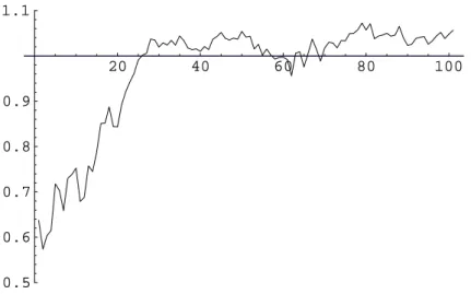
2.1 Estimated values for µ1 from MCEM 29

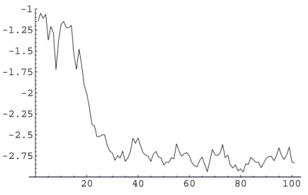
2.2 Estimated values for m from MCEM 30

2.3 Estimated values for M from MCEM 30

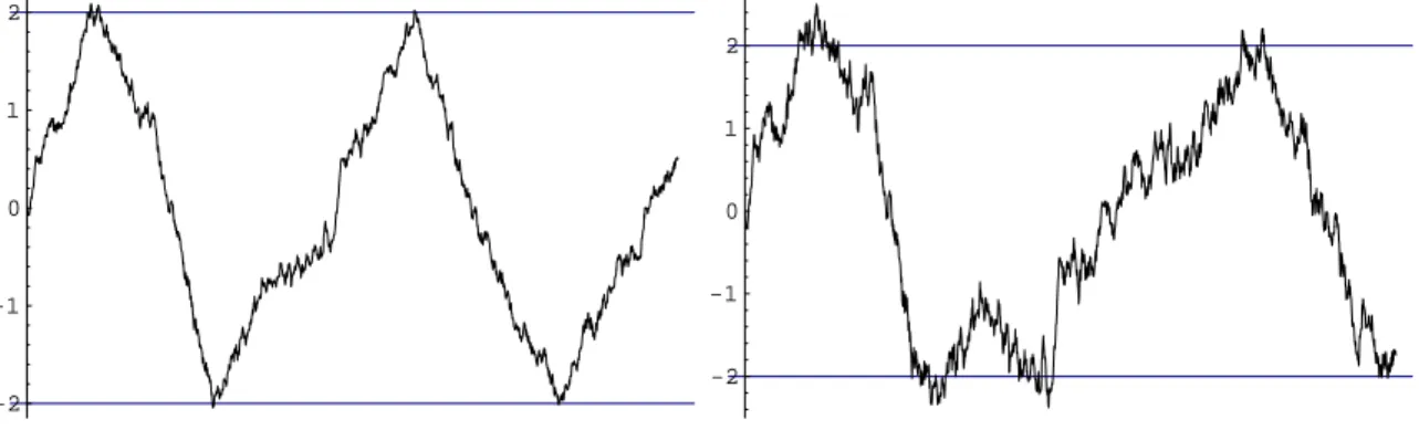
3.1 Two trajectories for the BMD threshold process 45

3.2 Trajectory for the BMD threshold process 47

3.3 Trajectory for the GBM threshold process 50

3.4 Trajectory for the OU threshold process 51

3.5 2004 daily prices from European Sustainable Equities-R fund 54

3.6 2004 daily prices from Parvest Europe Dynamic Growth fund 54

3.7 2005 daily prices from Converging Europe Bond fund 55

(14)

(15)

List of Tables

2.1 Mean and standard deviation for the estimates from MCEM 30

3.1 Estimates from BMD process with fixed ∆ in the [0,100_⌉ observation interval 45

3.2 Estimates from BMD process with fixed ∆ in the [0,500_⌉ observation interval 46

3.3 Estimates from BMD process with decreasing ∆ and fixed observation interval 46

3.4 Estimates from BMD process with decreasing ∆ and increasing observation

interval 47

3.5 Estimates from GBM process with decreasing ∆ and fixed observation interval 50

3.6 Estimates from GBM process with decreasing ∆ and increasing observation

interval 51

3.7 Estimates from O.U. process with decreasing ∆ and fixed observation interval 52

3.8 Estimates from OU process with decreasing ∆ and increasing observation interval 53

3.9 Threshold estimates from PF-European Sustainable Equities-R 54

3.10 Threshold estimates from Parvest Europe Dynamic Growth 55

3.11 Threshold estimates from Converging Europe Bond 55

(16)

(17)

Preface

The past decades have witnessed major developments in the field of statistical

infer-ence for diffusion processes and time series analysis. In the time series the assumptions

of linearity and stationarity have been abandoned and the study of nonlinear models

is increasing. One class of nonlinear models, called threshold models can be found in

[Tong, 1990], in this class the most popular is the threshold autoregressive model (T AR),

or T AR(m, p), where the process is divided into m regimes following in each regime an

AR model. Our goal is to extend the notion of threshold processes to continuous time

processes and obtain estimation methods for this kind of processes. A diffusion which

experiences a regime change upon crossing upper (M) and lower (m) levels will be our

generic model for the stochastic process. We want to study diffusions where changes in

the drift parameter have a consequence on the trend of the process, that is, we want to

consider diffusions with positive trend for some drift parameterµ1and with negative trend

for drift parameter µ2. For instance, the Brownian motion with drift is a diffusion of the

suggested type and the thresholds are introduced, in the model, in the following way. Let

us consider two thresholds, m and M, and suppose that we start with the process with

positive trend (driven byµ1) and the process continues in this first regime until it hits the

upper threshold M, at that time a change occurs and the process follows with negative

trend (driven byµ2) and continues in this second regime until it hits the lower threshold m, starting all over again in the first regime. We call the resulting process a continuous

time threshold model. Simple diffusion processes are often used for stochastic modelling

in many areas as physics, biology or economics. In many applications a continuous time

threshold model can be more useful than simple diffusion model, for instance in some

cool-ing (or heatcool-ing) system controlled by a thermostat we can observe this kind of behavior

in the temperature evolution see [Molina & et al., 2004], in a biological system where

the animal population increase until hits a threshold value that makes the population

dynamics to change (for instance the lack of food) and the population decreases until it

hits a lower threshold where the dynamics change (when the food is enough to support

a small population) and the population increases once again or in a financial context we

(18)

xviii PREFACE

can expect the price of some asset to have an increasing or decreasing dynamic between

two thresholds. All these models involve unknown parameters which need to be

esti-mated from observations of the processes. Different methods of estimation as maximum

likelihood, least squares or martingale estimating functions are well studied for diffusion

models. However, for thresholds diffusions models there are not (as to our knowledge)

(19)

CHAPTER 1

Overview on threshold model

1.1. Introduction

In the time series context the assumptions of linearity and stationarity have been

abandoned and the study of nonlinear models is increasing. One class of nonlinear models,

called threshold models can be found in [Tong, 1990], in this class the most popular is

the threshold autoregressive model (T AR), or T AR(m, p), where the process is divided

intomregimes following in each regime an ARmodel. This model can be represented by

the following equation:

(1.1) Yt=

m

X

i=1

(ai,0+ai,1Yt−1 +· · ·+ai,pYt−p+εi,t)I{ri−1≤Zt−1<ri},

where for each regimeithe nonlinear model is just ordinaryAR(p) process. The thresholds

are real numbers _−∞ =r0 < r1 < . . . < rm−1 < rm = +∞ and Zt−1 =Z(Y1, ..., Yt−1) is

the threshold variable that specifies the change in regime.

We want to study diffusions where changes in the drift parameter have a consequence

on the trend of the process, that is, we want to consider diffusions with positive trend

for some drift parameterµ1 and with negative trend for drift parameter µ2. Considering

two thresholds, m and M, and suppose that we start with the process with positive

trend (driven byµ1) and the process continues in this first regime until it hits the upper

threshold M, at that time a change occurs and the process follows with negative trend

(driven by µ2) and continues in this second regime until it hits the lower threshold m,

starting all over again in the first regime. This model can be specified by the following

equation:

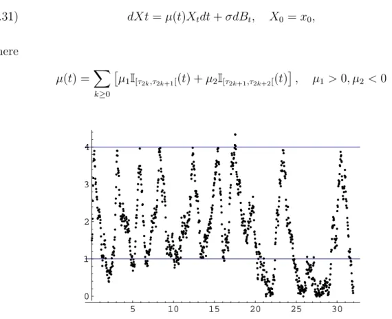
(1.2) dXt =a(µ(t), Xt)dt+b(σ, Xt)dBt,

with

µ(t) =X

k≥0

£

µ1I[τ2k,τ2k+1[(t) +µ2I[τ2k+1,τ2k+2[(t)

¤

,

where τ0 < τ1 < . . . < τj < . . . are the threshold hitting times, that is, τ2k+1 = inf{t > τ2k;Xt=M} and τ2k+2 = inf{t > τ2k+1;Xt =m} fork ≥0 and τ0 = 0.

(20)

2 1. OVERVIEW ON THRESHOLD MODEL

This thesis is mainly concerned with the estimation of the threshold parameters, m

and M, in the threshold diffusion process. The original contributions of this thesis are

contained in the next chapters. The thesis is organized as follows. The present chapter

continues with a review on the estimating procedures for the threshold models in the time

series context and in the diffusion context. Chapter 2 starts with an overview and some

results on hitting times for some diffusion processes and follows with the introduction of a

Monte Carlo Expectation Maximization type algorithm to estimate the parameters of the

Brownian motion with drift threshold model, from discrete observations of the process,

finishing with an implementation of the algorithm. In chapter 3, we start

implement-ing a conditional least squares estimation procedure for the Brownian motion with drift

threshold model, with decreasing step ∆n and knowing the regime for each observation,

after that we implement the procedure with unknown regimes. Finally, we generalize the

estimation procedure to more general threshold models as the ones built, for example,

from the Ornstein-Uhlenbeck and the geometric Brownian motion processes. For all the

estimating procedures presented, simulation studies are carried out and the results are

presented. In the end the procedure is also implemented with real data. Overall

con-clusions are presented in the end, along with some general comments on the estimation

methods and suggestions for possible extensions and future research.

1.2. Overview on TAR models

The objective of this overview is to look at some estimating procedures and relevant

questions in time-series threshold models. The threshold autoregressive model (1.1) can

be written as,

Yt=

            

a1,0+a1,1Yt−1+· · ·+a1,pYt−p+ε1,t, if Zt< r1 a2,0+a2,1Yt−1+· · ·+a2,pYt−p+ε2,t, if r1 ≤Zt< r2

· · ·

am,0+am,1Yt−1+· · ·+am,pYt−p+εm,t, if rm−1 ≤Zt

with p the order of the autoregression and m the number of regimes. One particular

well known case is the self-exciting threshold autoregressive model (SET AR), where the

threshold variable Zt is replaced by some lagged value of Yt that is Zt = Yt−d and d is

called the delay. For the threshold model, with Ai = (ai,0, ai,1, ..., ai,p), for i = 1, ..., m, r = (r1, ..., rm−1) and θ = (A1, ..., Am, r), the usual estimation procedure is conditional

(21)

1.2. OVERVIEW ON TAR MODELS 3

minimizes the conditional sum of squared errors,

LN(θ) = N

X

t=p

(Yt−Eθ[Yt|Ft−1])2,

with (F_t_{) the natural filtration and} _N _{the number of observations.} The minimization is done in two steps.

(1) For fixed r, we can get by ordinary least squares (OLS) values for ˆAi,N(r), i =

1, ..., mand write

SN(r) = m

X

i=1

Si,N( ˆAi,N, r)

whereSi,N( ˆAi,N, r) =PN_t=p

³

(Yt−Aˆi,N|Y)2I{ri−1≤Zt<ri}

´

,._|.stands for inner prod-uct andY = (1, Yt−1, ..., Yt−p).

(2) Then we choose ˆrN that minimizes SN(r), that is

(1.3) ˆrN = arg min

r SN(r)

and finally we put

ˆ

Ai,N = ˆAi,N(ˆrN), i= 1, ..., m.

Usually, it is assumed thatr_∈R with R bounded set, and in the SET ARcase the delay parameterdis introduced and a double grid (overdand r) is introduced in (1.3). For the

case of SET AR model with m= 2,

(1.4) Yt =

  

a1,0+a1,1Yt−1 +· · ·+a1,pYt−p+ε1,t, if Yt−d ≤r a2,0+a2,1Yt−1 +· · ·+a2,pYt−p+ε2,t, if Yt−d > r

where εi,t =ciεt with εt i.i.d. zero mean and unity variance, using the same estimation

procedure (CLS), fixing r and d and performing a grid search Chan, in [Chan, 1993],

showed that when the autoregressive function is discontinuous, that is, when _∃W∗ ₌

(1, wp−1, wp−2, ..., w0), with wp−d = r, such that (A1−A2)|W∗ 6= 0, the CLS estimator

ˆ

θN of θ is consistent. Moreover, in the same paper, the author shows that ˆrN is N

consistent andN(ˆrN −r) converges in distribution toM−, where [M−, M+[ is the unique

random interval over which a compound Poisson process attains its global minimum.

Furthermore,N(ˆrN −r) is asymptotically independent of

√

N( ˆA1−A1,Aˆ2−A2) and the

latter is asymptotically normal with the same distribution as that for the case when r is

known. Still in the SET AR(2, p) case, when the autoregressive function is continuous,

(22)

equivalent way, a1,i =a2,i for 1 ≤i 6=d≤ p and a1,0 +ra1,d =a2,0+ra2,d, that is, when

(1.4) can be written as

Yt =a0+ p

X

j=1,6=d

ajYt−j+

 



a1,d(Yt−d−r) +ε1,t if Yt−d ≤r a2,d(Yt−d−r) +ε2,t if Yt−d > r

where a0 = a1,0 +ra1,d and aj = a1,j = a2,j for j 6= d, Chan and Tsay, in the paper

[Chan & Tsay, 1998], show that theCLSestimator, ˆθN ofθ, is yet consistent. However,

ˆ

rN is now

√

N consistent and

√

N(ˆθN −θ) is asymptotically N(0, U−1V U),

where U =E[HtHtT] and V =E[e2tHtHtT]. With et(θ) = Yt−Eθ[Yt|Ft−1] and Ht(θ) =(−1,−Yt−1, ...,−Yt−d+1,−(Yt−d−r)−,−(Yt−d−r)+, ...,−Yt−p,

a1,dI{Yt−d≤r} +a2,dI{Yt−d>r})

T

the partial derivatives of et(θ) with respect to θ, where (y)− = min(y,0) and (y)+ =

max(y,0).

Hansen in a sequence of papers involving threshold models, studies several models. For

instance, in [Hansen, 2000] the author develops asymptotic theory for the distribution

of the regression estimates from the regression model, whenm = 2,

Yt=

  

AT

1Xt+εt, Zt≤r AT

2Xt+εt, Zt > r ,

with Xt = (1, X1,t, X2,t, ..., Xp,t), and when the regression errors form a martingale

dif-ference sequence. The estimation procedure is the same (CLS) and the fundamental

difference between the assumptions in [Hansen, 2000] and the other authors is that he

makes the assumption that

A2−A1 =cN−α,

that is, a decreasing threshold effect, with c₆= 0 and 0< α <1/2. Getting,

N1−2α(ˆrN −r)→d ωT

where

ω= c

T_{V c}

(cT_Dc₎2_f and T = arg max_s_∈R

·

−1₂|s_|+W(s)

¸

(23)

With, D=D(r) when D(s) =E[XtXtT|Zt=s],V =V(r) when V(s) = E[XtXtTε2t|Zt= s],f =f(r) when f(z) is the density of Zt and

W(s) =

         W1

−s, s <0

0, s = 0

W2

s, s >0 ,

whereW1

u and Wu2 are independent standard Brownian motion. The distribution forT is

known and given by,

P[T _≤x] = 1 +

r

x

2πexp

³

−x₈´+3

2exp(x)φ

µ −3 √ x 3 ¶ − µ

x+ 5 2 ¶ φ µ − √ x 2 ¶

whenx_≥0 and φcumulative standard normal distribution function. For x <0, P[T _≤ x] = 1₋P[T _{≤ −}x].

In [Hansen, 2000], the author also builds likelihood ratio tests to test the hypothesis

H0 :r =r0 under the assumption that εt are i.i.d. N(0, σ2). For the drift parameters in

the regression, he shows that, with ˆθ= ( ˆAT

1,AˆT2)T and θ = (AT1, AT2)T,

√

N(ˆθ₋θ)_→d N(0, Vθ),

whereVθ is the standard asymptotic covariance matrix as if r were fixed and known.

Earlier, in [Hansen, 1997] the author proved similar results about the asymptotic

distribution of the threshold and the likelihood ratio test for the T AR(2, p) model, he

also reviews the test for linearity suggested in [Hansen, 1996] to test the linear model

against the threshold model and the same kind of test is studied in [Hansen, 1999].

In the paper [Hansen & Seo, 2002] the authors provide an estimation procedure

for threshold co-integration in vector error-correction models with two regimes,

∆Yt =

  

AT

1Xt−1(β) +εt, wt−1(β)≤r AT

2Xt−1(β) +εt, wt−1(β)> r .

Where Yt is p-dimensional time series, I(1) (that is, each of the series is non-stationary

with unit root), which is co-integrated with cointegration vector β (so βTYt is stationary

orI(0)). Where wt(β) =βTYt,A is k×pmatrix and

Xt−1(β) = (1, wt−1(β),∆Yt−1, ...,∆Yt−l).

The errorsεt are assumed to form a martingale difference sequence with finite covariance

(24)

authors implement maximum likelihood estimation (M LE) of the threshold model. The

Gaussian likelihood is

L_N₍_A₁_{, A}₂_,_Σ_{, β, r}_{) =}₋N

2 log|Σ| − 1 2

N

X

t=1

εt(A1, A2,Σ, β, r)TΣ−1εt(A1, A2,Σ, β, r),

where

εt(A1, A2,Σ, β, r) = ∆Yt−AT1Xt−1(β)I{wt−1(β)≤r}−A T

2Xt−1(β)I{wt−1(β)>r}.

The M LE ( ˆA1,Aˆ2,Σˆ,β,ˆ rˆ) are the values that maximize LN(A1, A2,Σ, β, r), and the

proposed estimation procedure is the following:

(1) Form a grid forβ and r.

(2) For each value ofβ and r in the grid, calculate ˆA1(β, r), ˆA2(β, r) and ˆΣ(β, r) as

the constrained M LE for (A1, A2,Σ) (it coincides with OLS estimation).

(3) Find ( ˆβ,rˆ) as the values of (β, r) which yield the lowest value of

log_|Σ(ˆ β, r)_|

this is because the likelihood function is

L_N₍_{β, r}_{) =}L_N_{( ˆ}_A₁₍_{β, r}₎_,_Aˆ₂₍_{β, r}₎_,_Σ(ˆ _{β, r}₎_{, β, r}_{) =} ₋N

2 log|Σ(ˆ β, r)| −

N p

2 .

(4) Finally, set

ˆ

Σ = ˆΣ( ˆβ,rˆ), Aˆ1 = Â1( ˆβ,rˆ) and Â2 = Â2( ˆβ,rˆ).

Another process is studied by Tsay, in [Tsay, 1998], where the author considers a

multivariate (open-loop) threshold regression model,

(1.5) yt=cj +

p

X

i=1

φj_iyt−i+ q

X

i=1

β_ijxt−i+εjt, if rj−1 < zt−d ≤rj

withj = 1, ..., s,cj constant vectors,yand xare kand v dimensional, respectively. Given

observations _{yt, xt, zt}, t = 1, ..., N the author provides a test to detect the threshold

nonlinearity of yt. Writing the linear model in a regression framework,

y_tT =X_tTφ+εT_t, t =h+ 1, ..., N,

whereXt = (1, ytT−1, ..., ytT−p, xtT−1, ..., xTt−q)T,φis the parameter matrix andh= max(p, q, d).

The threshold variable takes values inS =_{zh+1−d, ..., zn−d}, denotingz(i) the i-th

(25)

based in the increasing order of the threshold variablezt−d is

(1.6) y_t(i)+dT =X_t(i)+dT φ+εT_t(i)+d, i= 1, ..., N ₋h.

To built the test the author uses predictive residuals. The idea is simply, ifytis linear then

the recursive LS estimator of (1.6) is consistent and the predictive residuals approach

white noise and are uncorrelated with the regressor Xt(i)+d. On the other hand, if yt

follows a threshold model, the predictive residuals will no longer be white noise because

the recursive LSE is biased and would be correlated with the regressor. The author

also generalizes in a similar way the results of [Chan, 1993] and [Hansen, 2000] about

the consistency of the CLS estimator of the parameters in model (1.5), and deduces the

asymptotic normal distribution for the slope parameters.

The estimation of threshold parameters and confidence intervals when the model

is SET AR(m, p) with discontinuous autoregressive function, is considered in the paper

[Kapetanios, 2003]. Using a different approach, the author proposes the use of

general-ized method of moments (GM M), specially in small samples. Using moment conditions

of the form

E[zj,t(r)εt] =E[ztI{rj−1≤Yt−d<rj}εt] = 0

wherezt are variables that provides extraneous information about the threshold

parame-ters. The author considers the loss function,

(1.7) Loss(Y;r) = ¯m(y;r)Tm¯(y;r)

where

¯

m(y, r)j =

1

N

X

i∈Γj(r)

zj,t(r)ˆεt(r),

r = (r1, ..., rm−1)T and Γj(r) denotes the set of observations for which the j-th moment

condition is specified to hold and ˆεt are the regression residuals. The author proves that

the estimator, ˆr, of the threshold parameter defined by the minimization of Loss(Y;r)

is consistent. The author also suggests the use of bootstrap (and sub-sampling) for

con-struction of standard errors and confidence intervals for the threshold parameter.

The model SET AR(2, p), is considered in [Gonzalo & Wolf, 2005] and the

pro-posed solution for inference about the threshold parameter is sub-sampling when the

estimation procedure for the model parameters is, once more, CLS. The basis of

(26)

sampling distribution of ˆrN, properly normalized. With

JN(u) =P[Nβ(ˆrN −r)≤u]

for some positive β, the sub-sampling approximation to JN(u) is defined by

LN,b(u) =

1

N ₋b+ 1

N_X−b+1

a=1

I_{_bβ_(ˆ_r

b,a−ˆrN)≤u},

where the integer 1< b < N is the block size and ˆrb,a= ˆr(Ya, ..., Ya+b−1) is the estimator

of r computed in the sub-sample Ya, ..., Ya+b−1, that is, CLS estimation applied to the

sub-sample.

In the paper [Gonzalo & Pitarakis, 2002] the model of interest is the threshold

regression model, and the authors give conditions under which the threshold parameters

converge to the true value when the CLS procedure is used in the sequential estimation

of the parameters. Computer burden becomes substantial when m > 2 and to overcome

this problem the authors propose a sequential estimation procedure for the threshold

parameters. The authors consider at each step of the procedure a threshold regression

model with two regimes, and follow the CLS estimation with a slight difference. Instead

of estimating ˆrN as in (1.3), that is, ˆrN = arg minrSN(r) the authors define

(1.8) JN(r) =SN −SN(r)

whereSN is the sum of the square of the residuals when the model is supposed linear and

estimate ˆrN has

ˆ

rN = arg max

r JN(r).

The authors deduce the (non-stochastic) limit J_∞(r) of JN(r) and give conditions for the

convergence

ˆ

rN p

→r(1)

where r(1) ∈ {r1, ..., rm−1} is the threshold parameter that dominates all the others in

terms of their contribution for the maximization of J_∞(r). Writing ˆr_N(1) for this first estimate, the sequential procedure continues, a second threshold estimate, ˆr_N(2), is given by

ˆ

r(2)_N = arg max

r JN(r|rˆ (1) N )

with

JN(r|rˆ_N(1)) =J1,N(r|rˆ(1)_N )In_r<ˆ_r(1)

N

o₊_J_2,N₍_r_|_r_ˆ(1)

(27)

The objective functions J1,N and J2,N are of the same kind of (1.8) but are built when is

adjusted a threshold regression model with two regimes at each sub-sample, and where

the sub-samples are selected using the condition, on the threshold variable Z, Zt < ˆrN(1)

and Zt>ˆr(1)N , respectively. Then,

ˆ

r(2)_N _→p r(2)

and the procedure follows until all the thresholds are estimated. In this paper, the

au-thors also discuss the small sample behavior of the estimators, and provide an estimating

procedure for the number of regimes.

The Bayesian theory is also used for inference in T AR models as in the paper of

[Stramer & Lin, 2002]. The authors consider a SET AR(2, p1, p2), that is, they

con-sider a two regime SET AR model but where the autoregressive order is p1 in the first

regime andp2 in the second regime, that is,

Yt=

  

a1,0+a1,1Yt−1+· · ·+a1,pYt−p1 +c1εt, if Yt−d≤r a2,0+a2,1Yt−1+· · ·+a2,pYt−p2 +c2εt, if Yt−d> r

where εt is standard white noise. The authors consider the following prior distribution

for the parameters,

(i) Ap_i are independentN(0, v−_i 1Ii), i= 1,2 withIithe identity matrix andvi positive

scalar.

(ii) c2

i are independentIG(α, β) where IGdenotes the inverse gamma distribution.

(iii) r follows a U[a, b] (uniform distribution) where a and b are the 25% and 75%

empirical quantiles of the data.

(iv) d followsU(1, ..., D), a discrete uniform distribution for some positive integer D.

(v) pi are independent U(0, .., Ki) for some positive integer Ki, i= 1,2.

The authors then propose a reversible jump Markov-Chain-Monte-Carlo algorithm to

jump between models with differentp′_{s and for dealing with models with different values}

of d.

Some authors use wavelets for inference in threshold models as the case in the

pa-pers [Li & Xie, 1999] and [Ip, Wong, Li & Xie, 1999]. In the first paper the authors

assume theSET AR(m, p) model,

Yt= m

X

i=1

(28)

with _−∞< a < r1 <· · ·< rm−1 < b <∞, and introduce the function,

T(y1, ..., yp) = m

X

i=1

(ai,0+ai,1y1+· · ·+ai,pyp)I{ri−1≤yd<ri}.

They built pempirical wavelet coefficients for the functionT(.) and use its properties for

the estimation of the delayd, the number of regimesm and the threshold coefficients. For

instance, checking the ones that have large absolute values the d parameter is estimated.

By further checking the empirical wavelets corresponding to the time delay across the fine

scale levels, the thresholds and their levels are identified. Finally the authors show the

consistency of the estimators.

In the second paper, [Ip, Wong, Li & Xie, 1999], the estimators are built in the

same way, but the process considered is the open-loop threshold autoregressive model

(T ARSO)

Yt = m

X

i=1

(ai,0+ai,1Yt−1+· · ·+ai,pYt−p+bi,0Xt+· · ·+bi,qXt−q+εi,t)I{ri−1≤Xt−d<ri}.

Then, they define the function T for this process as

T(z) =

m

X

i=1

(ai,0+ai,1y1+· · ·+ai,pyp+bi,0xt+bi,1xt−1+· · ·+bi,qxt−q)I{ri−1≤xd<ri}

with z = (y1, ..., yp, x1, ..., xq), and proceed as in the case of the SET AR model.

One fundamental question considered in several papers, [Caner & Hansen, 2001],

[Bec, Guay & Guerre, 2008], [Gonzalo & Montesinos, 2004], [Hansen, 1996],

[Hansen, 1999], [Hansen & Seo, 2002], [Tsay, 1998], [Wong & Li, 2000], is the

question of testing for linearity, that is, the question of testing the linear model against

some kind of threshold model.

1.3. Overview on diffusion threshold models

As to our knowledge the only paper where a threshold diffusion process is considered,

is in [Freidlin & Pfeiffer, 1998]. In this paper the authors consider Brownian motion

with a drift that changes from positive (b1) to negative (b0) and use it to build a threshold

model where the upper threshold (x1) is not known and the lower threshold is zero. The

regimes in the threshold model are driven by the positive and negative drifts, the process

is supposed to be continuously observed and the estimation procedure relies on maximum

(29)

1.3. OVERVIEW ON DIFFUSION THRESHOLD MODELS 11

defined as the continuous solution of the equation

dXt=bi(t)dt+σdBt, X0 =x <0,

where

i(t) =

  

1, τ2k ≤t < τ2k+1

0, τ2k+1 ≤t < τ2k+2

when τ2k+1 = min{t > τ2k : Xt = x1} and τ2k+2 = min{t > τ2k+1 : Xt = 0}. The

authors define a cycle for the level 0 < h < x1 as the time interval [τ2k∗ , τ2k+2∗ [ with τ∗

2k+1 = min{t > τ2k∗ :Xt =h}, τ2k+2∗ = min{t > τ2k+1∗ :Xt= 0}, that is, the time interval

between two successive intersections of the trajectory Xt with the level x = 0 separated

by crossing of the levelh and defineNT,h as the total number of cycles for the trajectory

of Xt in [0, T]. Next, for each cycle k they observe Xk = maxτ∗

2k<t<τ2∗k+2Xt and define,

withX(i)the ith-order statistic of theNT,h cycle maxima, the estimator ofx1 as the value X(l(NT ,h)) that satisfies,

X(l(NT ,h))(NT,h−l(NT,h)) = max

1≤i≤NT ,h

X(i)(NT,h−i).

(30)

(31)

CHAPTER 2

MCEM-algorithm

In this chapter we start with a first section dedicated to hitting times for some diffusion

processes and the chapter follows with a second section where we use the information on

hitting times to build an Expectation-Maximization type algorithm to estimate the model

parameters in the Brownian motion with drift threshold model.

2.1. Hitting times distribution

In this section we start with hitting times for the Brownian motion and the Brownian

motion with drift processes. The results being known will be stated and the proofs will

be written in order to allow the generalization for some other processes, namely the

geometric Brownian motion process. Given a stochastic process X with right-continuous

paths, which is adapted to a filtration (F_t₎_t_≥₀ _{and considering a subset Γ} _∈ B₍R) of the state space of the process, the hitting time (in Γ) is defined as,

TΓ(ω) = inf{t ≥0;Xt(ω)∈Γ}.

In the following the hitting times of interest will be in some predefined level or threshold.

2.1.1. Standard Brownian motion. Let B = (Bt)t≥0 be standard Brownian

mo-tion andTb = inf{t≥0 :Bt =b}, b∈Rthe first hitting time of the level b by the process B. We want to study the distribution ofTb.

Definition 2.1. Define the running maximum, or the maximum to the date, Mt, of

the Brownian motion by: _∀t >0, Mt = sup0≤s≤tBs

First we suppose b >0, from the following proposition is easy to deduce the density

function forTb.

Proposition 2.2 ([Hida, 1980] or [Revuz & York, 1991]). The following

equal-ities hold for b_≥0 and t >0:

P[Tb ≤t] =P[Mt ≥b] = 2P[Bt ≥b]

(32)

14 2. MCEM-ALGORITHM

We obtain the distribution functionFTb,

FTb(t) = P[Tb ≤t] =P[Mt ≥b] = 2 √

2πt

Z +∞

b

e−y 2 2tdy=

= _√2 2πt

Z +∞

b

√

t

e−x22√tdx.

doing the substitution x= √y

t. By differentiation the density of Tb is obtained,

fTb(t) = b √

2πt3e

−b22t, t≥0, b >0.

In the case b <0, we need the following definition.

Definition 2.3. Define the running minimum, or the minimum to the date, mt, of

the Brownian motion by: _∀t >0, mt= inf0≤s≤tBs.

Corollary 2.4. The following equalities hold for b_≤0 and t >0:

P[Tb ≤t] =P[mt≤b] = 2P[Bt≥ −b].

Proof. If b <0 we have _{Tb ≤t}={mt ≤b}, but

{mt ≤b}=

½

inf

0≤s≤tBs ≤b

¾

=

½

− sup

0≤s≤t

(₋Bs)≤b

¾

=

½

sup

0≤s≤t

Bs ≥ −b

¾

,

because (₋Bt)t≥0 is also a Brownian motion starting at the origin, and by proposition 2.2

we have

P[mt≤b] =P[Mt≥ −b] = 2P[Bt≥ −b].

¤

For b <0 we have_{Tb ≤ t} ={mt ≤b}= 2P[Bt ≥ −b] then in this case the density

of Tb is given by

fTb(t) = −b √

2πt3e

−b2

2t, t≥0, b <0,

and so we can finally write the density forTb, b ∈R,

fTb(t) = |b_| √

2πt3e

−b2

2t, t ≥0.

The moment generating function for Tb is known and can be written as

ϕTb(α) =

Z +∞

0

|b_|e−αt

2πt3 e

−b2

2tdt =

Z +∞

0

|b_|

2πt3e

−b2+2αt2

2t dt=e−|b|

√

(33)

2.1. HITTING TIMES DISTRIBUTION 15

2.1.2. Brownian motion with drift µ. In this section we want to study the

hit-ting times for the Brownian motion with drift process and we follow the construction in

[Karatzas & Shreve, 1991]. Let us consider the Ito process given by,

dB˜t=dBt−µdt, t≤T, B˜0 = 0

for T _∈[0,+_∞[ andBt standard Brownian motion. We continue with, Tb = inf{t ≥ 0 : Bt=b}. Let,

Mt= exp

µZ t

0

µdBs−

1 2

Z t

0 µ2ds

¶

=eµBt−1₂µ2t_,

then by the Girsanov theorem ([Øksendal, 1998] or [Karatzas & Shreve, 1991]) we

define the measure Pµ _{in (Ω}_,_F T) by,

dPµ₌_M

TdP= exp

µ

µBT −

1 2µ

2_T

¶

dP

and w.r.t. Pµ_{, the process ˜}_B

t, t≤T is a Brownian motion. Then we say that, under Pµ, Bt=µt+ ˜Bt is a Brownian motion with driftµ.

Remark 2.5. We have that,

(1) (Mt)₀_≤_t_≤_T is a martingale w.r.t. (Ft)t≤T and P, ([Øksendal, 1998](Ex. 4.4)),

and so MTdP=MtdP inFt.

(2) Pµ_[_A_{] =}_E_[_I

AMt],∀A∈Ft because Pµ[A] =

R

ΩIAdP µ ₌R

ΩIAMtdP=E[IAMt].

With t fixed, on the set _{Tb ≤ t} ∈ Ft∩FTb = Ft∧Tb we have Mt∧Tb =MTb and the Optional Sampling theorem ([Karatzas & Shreve, 1991] or [Revuz & York, 1991])

with the remark imply

Pµ_[_T

b ≤t] =E

£

I_{_T_b_≤_t_}Mt

¤

=E£E[I_{_T_b_≤_t_}Mt|Ft∧Tb]

¤

=E£I_{_T_b_≤_t_}E[Mt|Ft∧Tb]

¤

=E£I_{Tb≤t}Mt∧Tb

¤

=E£I_{Tb≤t}MTb

¤

=E

·

I_{Tb≤t}exp

µ

µBTb − 1 2µ 2_T b ¶¸ =E ·

I_{_T_b_≤_t_}exp

µ

µb₋1

2µ 2_T b ¶¸ = Z t 0

eµb−12µ2sP[T_b ∈ds]

=

Z t

0

eµb−12µ2s√|b|

2πs3e

−b2

2sds=

Z t

0

|b_| √

2πs3e

−(b−2µss)2ds. (2.1)

SoTb has the density, under Pµ,

Pµ_[_T

b ∈dt] = | b_| √

2πt3e

(34)

Because, under Pµ_, _B

t =µt+ ˜Bt is a Brownian motion with drift µ, we can say that the

density of T_bµ is

fT_bµ(t) = | b_| √

2πt3e

−(b−2µtt)2, t >0,

with T_bµ= inf_{t:µt+Wt =b} wereWt is the standard Brownian motion. We will write B_tµ forµt+Bt and we get the moment generating function for Tbµ,

ϕT_bµ(α) =E[e−αT

µ b] =

Z +∞

0

e−αtfT_bµ(t)dt=eµb−|b|

√

µ2_+2α

, α >0.

If we consider a Brownian motion with driftµ but starting ata instead of 0, represented

as B_t,aµ , and because T_b,aµ = inf_{t : Bµ_t,a = b_} = inf_{t : B_tµ = b₋a_} = T_bµ₋_a we get the density

fTb,aµ (t) =

|b₋a_| √

2πt3e

−(b−a2−tµt)2, t >0,

and the moment generating function,

ϕT_b,aµ (α) = eµ(b−a)−|b−a|

√

µ2_+2α

, α >0.

2.1.3. Brownian motion with drift µ and diffusion coefficient σ. Let us

con-sider the Brownian motion with drift µand diffusion coefficient σ,

Btµ,σ =µt+σBt

with Bt the standard Brownian motion. Starting with

Bµ/σ_t = µ

σt+Bt,

then we have

Btµ,σ =σB µ/σ t .

But

T_bµ,σ = inf_{t:Btµ,σ =b}= inf

n

t :σBµ/σt =b

o

= inf

½

t :Btµ/σ = b σ

¾

=Tµ/σb σ

,

and because of what we have done in the last section, we obtain the density when B0µ,σ = a_⇔B₀µ/σ =a/σ

fT_b,aµ,σ(t) = | b₋a_| √

2πσ2_t3 e

−(b−₂a_σ−2µtt)2, t >0,

and, the moment generating function,

ϕT_b,aµ,σ(α) =e

µ(b−a)−|b−a|√µ2+2ασ2

(35)

2.1.4. Transformation of the Brownian motion with drift. Let us consider the

Brownian motion with drift, B_tµ,σ, we know the density for the first hitting time, T_b,aµ,σ. Define a new process by

Yt=g(Btµ,σ), Y0 =a,

for an invertible monotonous function g. Because

T_b,aY = inf_{t_≥0 :Yt=b}= inf{t≥0 :g(Btµ,σ) = b}

= inf©t_≥0 :B_tµ,σ =g−1(b)ª=T_gµ,σ−1_(b),g−1_(a),

we have the density for TY

b,a given by:

(2.2) f_TY

b,a(t) =

|g−1₍_b₎₋_g−1₍_a₎_|

√

2πσ2_t3 e

−(g

−₁₍b)−g−1(a)−µt)2

2σ2t , t >0,

and the moment generating function

ϕTY

b,a(α) = e

µ(g−1(b)−g−1(a))−|g−1(b)−g−1(a)|√µ2+2ασ2

σ2 , α >0.

Remark 2.6. When we consider the process Yt = g(Btµ,σ) by the Ito’s formula, we

get

(2.3) dYt=

·

g′¡g−1(Yt)

¢

µ+σ

2

2 g

′′¡_g−1₍_Y t)

¢¸

dt+σg′¡g−1(Yt)

¢

dBt,

and the results can be applied to the processes solution of this kind of s.d.e.

2.1.5. Geometric Brownian motion. If we consider the geometric Brownian

mo-tion, a positive process satisfying,

dXt=µXtdt+σXtdBt, X0 =a.

We know that the solution of the last s.d.e. is given by,

Xt=a e ³

µ−σ2

2 ´

t+σBt ,

we can then write

Xt=g

µ

Bµ−σ 2 2 ,σ t

¶

with

g(z) = aez, g−1(x) = ln³x

a

´

.

Then we can write, using (2.2), the density for the first hitting time of the geometric

Brownian motion,

fTX b,a(t) =

|ln(b)₋ln(a)_| √

2πσ2_t3 e

−

µ

ln(b)−ln(a)− µ

µ−σ₂2 ¶

t

¶2

(36)

and, the moment generating function,

ϕ_TX

b,a(α) = e

1 2 ·

ln(a)−ln(b)+2µ(ln(b)−ln(a))−|ln(b)−ln(a)|

√

8ασ2+(σ2−2µ)2

σ2

¸

, α >0.

2.1.6. Simple generalization. More generally, instead of starting with a Brownian

motion, we can think in the process solution of the SDE

dXt=α(t)dBt, X0 = 0,

that is,

Xt =

Z t

0

α(s)dBs,

where α(t) is a deterministic regular function. Our goal is to obtain the density for the

hitting times of such a process. We know that Xt is a time changed Brownian motion

Xt=BhXit with hXit=

Z t

0

α(s)2ds,

and we need a reflection principle for this kind of processes.

Proposition 2.7. Let Xt=

Rt

0 α(s)dBs, X0 = 0, α(s) continuous function and ∀t >

0, _hX_it≥t. With MtX = sup0≤s≤tXs and TbX = inf{t≥0;Xt =b} we have for b≥0

P[T_bX _≤t] =P[M_tX _≥b] = 2P[Xt≥b].

Proof. First observe that _{TX

b ≤t}={MtX ≥b} because Bt has continuous

trajec-tories and α is continuous. On the other hand we have

P[M_tX _≥b] =P[M_tX _≥b, Xt ≥b] +P[MtX ≥b, Xt< b]

because _{Xt≥b} ⊆ {MtX ≥b} we get

P[M_tX _≥b, Xt ≥b] =P[Xt≥b].

Because XTX

b =b we can write

P[M_tX _≥b, Xt< b] =P[TbX ≤t, Xt < b] =P[TbX ≤t, XTX

b +(t−TbX)−XTbX <0] and with s=t₋TX

b

XTX

b +s−XTbX =BhXi(T X b +s)−

B_hXiT X b

.

Taking into account that _hX_it is increasing and in {TbX ≤t}we have s >0, so

hX_i_TX

(37)

and with B Brownian motion and the hypotheses made we get

B_hXi₍T X b +s) −

B_hXiT X b ⊥

F_h_X_i T X b ⊇ F TX b . Then

XTX

b +s−XTbX ⊥ F_TX

b

and

P[M_tX _≥b, Xt< b] =P[TbX ≤t]P[XTX

b +s−XT X

b <0] = 1 2P[T

X b ≤t],

because X_TX

b +s−XT X

b has Normal distribution with zero mean. Finally,

P[MX

t ≥b] = 2P[Xt ≥b].

¤

In the same way as earlier we can get the distribution for TX

b = inf{t ≥ 0 : Xt = b_}, b_≥0, once B_hXit ∼N(0,hXit),

FTX

b (t) = P[M

X

t ≥b] = 2P[BhXit ≥b] = 2

p

2π_hX_it

Z +∞

b

e− y 2 2hXitdy =

= p 2

2π_hX_it

Z +∞

b

√

hXit

e−x22phXi_tdx,

doing the substitution

x= py

hX_it .

By differentiation we obtain the density of TX b ,

fTX b (t) =

b_hX_i′t

p

2π_hX_i3 t

e− b 2

2hXit, t≥0, b >0.

Forb <0 we have the following analogous result.

Corollary 2.8. With the same assumptions of the last proposition, and mX t =

inf0≤s≤tXs and TbX = inf{t≥0;Xt =b} we have for b <0 P[T_bX _≤t] =P[m_tX _≤b] = 2P[Xt ≥ −b].

Proof. It is enough to see,

{T_bX _≤t_}=_{mX_t _≤b_}=_{ inf

0≤s≤tXs ≤b}={₀sup_≤_s_≤_t(−Xs)≥ −b}

=_{sup

0≤s≤t

B_h−Xis ≥ −b}={sup

0≤s≤t

B_hXis ≥ −b}={M

X

t ≥ −b}.

By proposition 2.7,

(38)

¤

Becoming

(2.4) f_TX

b (t) =

|b_|hX_i′

t

p

2π_hX_i3 t

e− b 2

2hXit, t≥0, b∈R.

Remark 2.9. If we consider α(t)_≡1 thenXt=Bt, hXit=t and the last density is

just what we have computed in a previous section.

In order to generalize this result to a drifted process, let Yt be the solution of

dYt=−µα(t)dt+dBt, t ≤T, Y0 = 0

with α(t) as in proposition 2.7, Bt a Brownian motion. Then by Girsanov’s with

Mt = exp

µZ t

0

µα(s)dBs−

1 2

Z t

0

µ2α2(s)ds

¶

, t _≤T

we define the measure Q in (Ω,F_T_{) by,}

dQ=MTdP,

with respect to which

Yt =−µ

Z t

0

α(s)ds+Bt

is a Brownian motion, for t_≤T. Let

Xt=

Z t

0

α(s)dBs, X0 = 0, TbX = inf{t ≥0;Xt=b},

similarly to the case of the Brownian motion with drift, remark 2.5 and equation (2.1),

because Xt∈Ft, {TbX ≤t} ∈Ft and TbX ∈FTX b .

Q[T_bX _≤t] =EP

"

I_{_TX

b ≤t}exp

Ã

µ

Z TX b

0

α(s)dBs−

1 2µ

2Z T

X b

0

α2(s)ds

!#

=EP

·

I_{_TX

b ≤t}exp

µ

µX_TX b −

µ2

2 hXiTbX

¶¸

=

Z t

0 eµb−µ

2

2 hXisP[TX b ∈ds]

=

Z t

0 eµb−µ

2

2 hXis |b|hXi

′

s

p

2π_hX_i3 s

e− b 2 2hXisds =

Z t

0

|b_|hX_i′

s

p

2π_hX_i3 s

e−(b−2µhhXXiiss)2ds.

So the density w.r.t. Q of TX

b is given by,

fTX b (t) =

|b_|hX_i′

t

p

2π_hX_i3 t

e−(

b−µhXit)2

2hXit .

We can write,

Xt=

Z t

0

α(s)dBs =

Z t

0

α(s)dYs+µ

Z t

0

(39)

2.2. MCEM-ALGORITHM IN THE THRESHOLD MODEL 21

also w.r.t. Q, Yt is Brownian motion, and we can conclude that for the process solution

of the SDE

dXt=µα2(t)dt+α(t)dBt,

with Bt Brownian motion, we have

fTX b (t) =

|b_|γ′₍_t₎

p

2πγ3₍_t₎e

−(b−2µγγ((tt)))2_, _γ₍_t_{) =}

Z t

0

α2(s)ds.

Remark 2.10. Once more, writing α(t)_≡1 then Xt is just a Brownian motion with

driftµ,γ(t) =t and

fTX b (t) =

|b_| √

2πt3e

−(b−2µtt)2,

just as earlier for the Brownian motion with drift.

2.2. MCEM-algorithm in the threshold model

In this section we consider the Brownian motion with drift in order to built a threshold

model. Given two thresholds, m and M, and supposing that the change occurs only in

the drift coefficient we built a threshold model. Starting the process with a positive

trend (driven by µ1 >0), the process continues in this first regime until it hits the upper

threshold M, at that time a change occurs and the process follows with negative trend

(driven by µ2 < 0) and continues in this second regime until it hits the lower threshold m, starting all over again in the first regime. To estimate the thresholds m and M

and the drift parameters we use an Expectation-Maximization (EM) type algorithm for

incomplete data because we will work with observed data from the process but this data

do not include observations of the threshold hitting times.

Let us consider the following model:

dXt=µ(t)dt+σdBt, X0 =x0 ∈[m, M[,

where

µ(t) =X

k≥0

£

µ1I[τ2k,τ2k+1[(t) +µ2I[τ2k+1,τ2k+2[(t)

¤

, µ1 >0, µ2 <0

where 0 =τ0 < τ1 < . . . < τk < . . . are the threshold hitting times. That is, giving two

thresholds m and M, τ1 is the time needed for the Brownian motion with drift µ1 to go

fromx0 toM,τ2−τ1 is the time needed for the process with driftµ2 go fromM tomand,

more generally,τi−τi−1 is the time needed for the process to go from one threshold to the

other. We supposeσ is known and we want to estimate θ= (µ1, µ2, m, M). Suppose that

(40)

with ∆ =tj−tj−1 andtj =j∆ forj = 1, ..., n. In both regimes the Brownian motion with

drift is used to build the threshold model as explained before, however the resulting process

is not a Brownian motion with drift in each of the regimes. Notice that, in the Brownian

motion with drift process we have Xj+1−Xj ∼ N(µ∆, σ2∆) but in the corresponding

threshold process this is not true, even if we know that is no change in regime between

the observation times. The transition densities are not known for the threshold process

and for that reason we use what we think that is a natural approximation, the transition

densities of the Brownian motion with drift process. In the next chapter we will return

again to the problem of the threshold process not being Brownian motion with drift in

each regime. If we consider Brownian motion with drift µ1 in the first regime of the

process and Brownian motion with drift µ2 in the second regime, then p1 and p2, the

transition densities in regime 1 and 2, are

p1(∆, xi, xi+1;µ1) =

1 √

2πσ2_∆exp

µ

−(xi+1−xi−µ1∆)

2

2σ2_∆

¶

p2(∆, xi, xi+1;µ2) =

1 √

2πσ2_∆exp

µ

−(xi+1−xi−µ2∆)

2

2σ2_∆

¶

.

The hitting times τ1, ..., τk are not observed and their number in the time interval [0, T] is

given by some random variableK. The densities for the difference between two consecutive

hitting times τ1, ..., τk are known (subsection 2.1.3), and given by:

fT1(τ1;µ1, M) =

M ₋x0

p

2πσ2_τ3 1

exp

µ

−(M −x0−µ1τ1)

2

2σ2_τ 1

¶

,

for i= 2,4,6, ...,

fTi−Ti−1(τi−τi−1;θ) =

M₋m

p

2πσ2₍_τ

i−τi−1)3

exp

µ

−(m−M −µ2(τi−τi−1))

2

2σ2₍_τ

i−τi−1)

¶

,

and for i= 3,5,7, ...,

fTi−Ti−1(τi−τi−1;θ) =

M₋m

p

2πσ2₍_τ

i−τi−1)3

exp

µ

−(M−m−µ1(τi−τi−1))

2

2σ2₍_τ

i−τi−1)

¶

.

Because the hitting times process is Markov, we can write the joint density for k hitting

times as,

fT1,...,Tk(τ1, ..., τk;θ) =

M ₋x0

p

2πσ2_τ3 1

exp

µ

−(M −x0−µ1τ1)

2

2σ2_τ 1

¶_Yk

i=2

M ₋m

p

2πσ2₍_τ

i−τi−1)3

×

[(k−1)/2]

Y

i=1

exp

µ

−(M −m−µ1(τ2i+1−τ2i))

2

2σ2₍_τ

2i+1−τ2i)

¶[k/2]

Y

i=1

exp

µ

−(m−M −µ2(τ2i−τ2i−1))

2

2σ2₍_τ

2i−τ2i−1)

¶

(41)

where [v] = maxl∈N{l ≤v}. To get estimators for the drift and the threshold parameters we will use a Monte Carlo EM algorithm, because the hitting times are not observed and

we will use Monte Carlo simulation in the expectation step.

To implement the algorithm, we will augment the data X1, ..., Xn by considering the

hitting timesT1, ..., TK in order to write the complete likelihood function,

LKc (ω) = +∞

X

k=1

Lc(x1, ..., xn, τ1, ..., τk;θ)I{K=k}(ω)

with K the random variable that represents the number of hitting times in the interval

[0, T] (we don’t consider the term were K = 0 because in that case there is no change

in regime in [0, T]). Conditionally on the hitting times the process Xt is Markov and we

have

Lc(x1, ..., xn, τ1, ..., τk;θ) = fX1,...,Xn,T1,...,Tk(x1, ..., xn, τ1, ..., τk;θ) =fX1,...,,Xn|T1,...,Tk(x1, ..., xn|τ1, ..., τk)fT1,...,Tk(τ1, ..., τk;θ)

=

j1−1

Y

i=0

p1(∆, xi, xi+1)p1(τ1−tj1, xj1, M)p2(tj1+1−τ1, M, xj1+1) j2−1

Y

i=j1+1

p2(∆, xi, xi+1)

×p2(τ2−tj2, xj2, m)p1(tj2+1−τ2, m, xj2+1)· · ·p[1+mod(k+1,2)](τk−tjk, xjk, ⋆)

×p[1+mod(k,2)](tjk+1−τk, ⋆, xjk+1)

n−1

Y

i=jk+1

p[1+mod(k,2)](∆i, xi, xi+1)

× pM −x0

2πσ2_τ3 1

exp

µ

−(M −x0−µτ1)

2

2σ2_τ 1

¶_Yk

i=2

M₋m

p

2πσ2₍_τ

i −τi−1)3

×

[(k−1)/2]

Y

i=1

exp

µ

−(M −m−µ1(τ2i+1−τ2i))

2

2σ2₍_τ

2i+1−τ2i)

¶[k/2]

Y

i=1

exp

µ

−(m−M −µ2(τ2i−τ2i−1))

2

2σ2₍_τ

2i−τ2i−1)

¶

,

where for alli= 1, ..., k, ji ∈ {1, ..., n−1} is, such thatτi ∈]tji, tji+1[ andj1 < j2 <· · ·< jk. With ⋆=m×mod(k+ 1,2) +M ×mod(k,2) and mod(a, b) is the remainder of the

integer division of a byb. Then we define the complete log-likelihood in a similar way,

log(LK_c )(ω) =

+∞

X

k=1

(42)

with

log(Lc(x1, ..., xn, τ1, ..., τk;θ)) =

=₋

Ã_j1₋₁ X

i=0

(xi+1−xi−µ1∆)2

2σ2_∆ +

j2_X−1 i=j1+1

(xi+1−xi−µ2∆)2

2σ2_∆ +· · ·

+

n−1

X

i=jk−1

(xi+1−xi−µ[1+mod(k,2)]∆)2

2σ2_∆ +

[(k+1)/2]

X

i=1

(M ₋xj2i−1 −µ1(τ2i−1−tj2i−1)) 2

2σ2₍_τ

2i−1−tj2i−1)

+

[(k+1)/2]

X

i=1

(xj2i−1+1−M −µ2(tj2i−1+1−τ2i−1))

2

2σ2₍_t

j2i−1+1−τ2i−1)

+

[k/2]

X

i=1

(m₋xj2i −µ2(τ2i−tj2i))

2

2σ2₍_τ

2i −tj2i)

+

[k/2]

X

i=1

(xj2i+1−m−µ1(tj2i+1−τ2i))

2

2σ2₍_t

j2i+1−τ2i)

 + log

Ã

M ₋x0

p

2πσ2_τ3 1

!

− (M −x0−µ1τ1)

2

2σ2_τ 1 + k X i=2 log Ã

M ₋m

p

2πσ2₍_τ

i−τi−1)3

!

−

[(k−1)/2]

X

i=1

(M₋m₋µ1(τ2i+1−τ2i))2

2σ2₍_τ

2i+1−τ2i) − [k/2]

X

i=1

(m₋M ₋µ2(τ2i−τ2i−1))2

2σ2₍_τ

2i−τ2i−1)

,

apart from a term not involving θ.

2.2.1. E-step. Using the EM algorithm we need in the p-iteration of the E-step to

compute the expectation of the log-likelihood of the augmented data given the observed

data and current value θp = (µ1,p, µ2,p, mp, Mp), that is

Q(θ, θp) =Eθp

£

log¡LK_c (X1, ..., Xn, T1, ..., TK)

¢

|X1, ..., Xn

¤

.

We will approximate this expectation conditionally on the observed data through Monte

Carlo.

Concretely, we simulate replicates τl

1, ..., τkll, l = 1, ..., L, of T1, ..., TK and weight the replicates using importance sampling. Notice that, for each l _{∈ {}1, ..., L_} we draw the sequence τl

1, ..., τkll from

fT1,...,T_kl(τ1, ..., τkl;θp) =fT1(τ1;µ1,p, Mp)fT2−T1(τ2−τ1;θp)fT_kl−T_kl−1(τkl−τkl−1;θp)

in a sequential way. That is, we drawsl

1 fromfT1 taking τ1l =sl1 then drawsl2 fromfT2−T1

taking τl

2 = τ1l +sl2 and so on (while we are in the [0, T] interval). In this way we are

(43)

Finally, we can approximate the conditional expectation of the log-likelihood of the

augmented data writing,

(2.5) E_θ_p£log¡LK_c ¢_|X1, ..., Xn

¤

≈ _L1

L

X

l=1

log¡Lkl

c (X1, ..., Xn, τ1l, ..., τkll)

¢

×wl,

where the weightwl _{is such that,}

wl _∝fX1,...,Xn|T1,...,T_kl(x1, ..., xn|τ

l

1, ..., τkll)fT1,...,Tkl(τ

l

1, ..., τkll).

2.2.2. M-step. In the M-step of the algorithm we want to maximize Q(θ, θp) with

respect to θ. Because of what we have done so far, this is just get the value of θ that

maximizes,

QL(θ, θp) =

1

L L

X

l=1

log¡Lkl

c (X1, ..., Xn, τ1l, ..., τkll)

¢

×wl.

We start by differentiating QL(θ, θp) with respect to θ and solving,

dQL(θ, θp)

dθ = 0⇔

      

∂QL(θ,θp)

∂µ1 ∂QL(θ,θp)

∂µ2 ∂QL(θ,θp)

∂m ∂QL ∂M        =        0 0 0 0       

Forµ1,

∂QL(θ, θp) ∂µ1 = 1 L L X l=1 "

∂log¡Lkl

c (x1, ..., xn, τ1l, ..., τkll;θ)

¢

∂µ1

wl

#

Equating to zero we get,

(2.6) µ1

Ã _L

X

l=1

£

a1,lwl

¤! − L X l=1 £

b1,lwl

¤

= 0,

with

a1,l = ∆



j₁l +

[(kl_X−1)/2]

i=1

(j_2i+1l ₋j_2il ₋1) + (n₋j_kl_l₋1)mod(kl+ 1,2)



+ 2τ₁l

+ 2

[(kl_X−1)/2]

i=1

(τ_2i+1l ₋τ_2il ) +τ_kl_lmod(kl+ 1,2) + [k_Xl/2]

i=1

(t_jl

2i+1−tj2li−1)−tj_kll mod(kl,2), b1,l =xnmod(kl+ 1,2)−2x0+M(2[(kl+ 1)/2])−m(kl−1),

and using the fact that tj =j∆. For µ2 we get,

(2.7) µ2

Ã _L

X

l=1

£

a2,lwl

¤! − L X l=1 £

b2,lwl

¤

(44)

with

a2,l = ∆

 

[k_Xl/2]

i=1

(j_2il ₋j_2il₋₁₋1) + (n₋j_kl_l₋1)mod(kl,2)



+ 2

[k_Xl/2]

i=1

(τ_2il ₋τ_2il₋₁)

−τ_kl_lmod(kl,2) +tjl

1+1+

[(kl−1)/2]

X

i=1

(t_jl

2i+1+1−tj2li)−tj_kll mod(kl+ 1,2), b2,l =xnmod(kl,2) +m(2[kl/2])−M kl.

Form we get the equation,

m2

Ã _L

X

l=1

h

(U_ml _p+Wl)wli

! +m Ã _L X l=1 h

(₋M(U_ml _p+ 2Wl)₋V_ml_p +µ1(kl−1)−µ2(2[kl/2]))wl

i! + Ã _L X l=1 h

(M(V_ml_p₋µ1(kl−1) +µ2(2[kl/2]))−σ2(kl−1) +M2Wl)wl

i!

= 0.

(2.8)

With

Ul mp =

[k_Xl/2]

i=1

∆ (τl

2i−tjl

2i)(tj2li+1−τ

l 2i) V_ml_p =

[kl/2]

X

i=1 xjl

2i(tj2li+1−τ

l

2i) +xjl

2i+1(τ

l 2i−tjl

2i) (τl

2i−tjl

2i)(tj2li+1−τ

l 2i) Wl =

kl

X

i=2

1

τl i −τil−1

.

Doing the same with respect to M we get,

M3

Ã _L

X

l=1

·µ

−UMl p−W

l

−_τ1l 1

¶

wl

¸!

+M2

Ã _L

X

l=1

h³

(x0+m)UMl p+V

l Mp

+µ1(2[(kl+ 1)/2])−µ2kl+

2x0+m τl

1

+ (x0+ 2m)Wl

¶ wl ¸¶ +M Ã _L X l=1 ·µ

−x0mUMl p−(x0+m)(V

l

Mp+µ1(2[(kl+ 1)/2])−µ2kl) +σ

2_k l−

x2

0+ 2mx0 τl

1

−(m2+ 2x0m)Wl

¢

wl¤¢+

Ã _L

X

l=1

h³

x0m(VMlp+µ1(2[(kl+ 1)/2])−µ2kl

+x0

τl 1

+mWl)₋σ2(m+ (kl−1)x0)

¶

wl

¸¶

= 0,

(45)

with,

Ul Mp =

[(kl_X+1)/2]

i=1

∆ (τl

2i−1−tjl

2i−1)(tjl2i−1+1−τ l 2i−1)

;

V_Ml_p =

[(kl+1)/2]

X

i=1 xjl

2i−1(tjl2i−1+1−τ l

2i−1) +xjl

2i−1+1(τ l

2i−1−tjl

2i−1)

(τl

2i−1−tjl

2i−1)(tj2li−1+1−τ l 2i−1)

.

Finally, we only need to solve the equations to getθp+1 and start the (p+ 1)-iteration of

the algorithm. If we consider the special case µ1 = −µ2 = µ, then the equations are as

following. Forµ

µ

Ã _L

X

l=1

£¡

n∆ +τ_kl_l¢wl¤

!

−

L

X

l=1

[((2kl−2)(M −m) + 2(M −x0)

+(M₋xn)mod(kl,2) + (xn−m)mod(kl+ 1,2))wl

¤

= 0,

(2.10)

form,

m2

Ã _L

X

l=1

h

(U_ml _p+Wl)wli

! +m Ã _L X l=1 h

(₋M(U_ml _p+ 2Wl)₋V_ml_p +µ[2[kl/2] +kl−1])wl

i! + Ã _L X l=1 h

(M(V_ml_p₋µ[2[kl/2] +kl−1])−σ2(kl−1) +M2Wl)wl

i!

= 0,

(2.11)

and for M we get,

M3

Ã _L

X

l=1

·µ

−UMl p−W

l

−_τ1l 1

¶

wl

¸!

+M2

Ã _L

X

l=1

h³

(x0+m)UMl p+V

l Mp

+µ(2[(kl+ 1)/2] +kl) +

2x0+m τl

1

+ (x0+ 2m)Wl

¶ wl ¸¶ +M Ã _L X l=1 ·µ

−x0mUMl p−(x0+m)(V

l

Mp+µ(2[(kl+ 1)/2] +kl)) +σ

2_k l−

x2

0+ 2mx0 τl

1

−(m2+ 2x0m)Wl

¢

wl¤¢+

Ã _L

X

l=1

h³

x0m(VMlp +µ(2[(kl+ 1)/2] +kl)

+x0

τl 1

+mWl)₋σ2(m+ (kl−1)x0)

¶

wl

¸¶

= 0.

(2.12)

Remark 2.11. To start the algorithm we need initial values for µ1, µ2, m and M.

Brownian Motion with Drift Threshold Model

Pedro Jos´

e dos Santos Palhinhas Mota