Productive performance and economic evaluation of tilapia stocked in
different times of the year
Jesaias Ismael da Costa1*, Omar Jorge Sabbag2, Luiz Marques da Silva Ayroza3, Maria Inez Espagnoli Geraldo Martins1
1 Universidade Estadual Paulista “Júlio de Mesquita Filho”, Centro de Aquicultura, Jaboticabal, SP, Brazil. 2 Universidade Estadual Paulista “Júlio de Mesquita Filho”, Ilha Solteira, SP, Brazil.
3 Agência Paulista de Tecnologia dos Agronegócios, Instituto de Pesca, São Paulo, SP, Brazil.
ABSTRACT - This study aimed to determine production cycles based on the stocking period and the influence of the cycles on productive performance indices, production costs, and profitability. The present study was carried out on a fish farm located in Palmital - SP, Brazil, which consists of 2706 m3 of net cages with an annual production of 400 tons of tilapia and regular harvests throughout the year. Production data, investment and expenditures were obtained by using a semi-structured questionnaire to calculate the total operational costs and profit indices. All monetary values of invested items have been corrected by the General Price Index (GPI) for December 2014. Three rearing phases were identified and characterized as the nursery, pre-finishing, and finishing phases. The production cycle is between 195 and 270 days and the profitability index is between 15.08 to 26.09%, in which the best production scenario is found when carrying out all of the rearing stages (nursery, pre-finishing, and finishing) in high temperatures. The stocking fish in low temperatures increases the production time by 38.46%. The extend production time allow the producer to regularly offer the product and have more flexibility on the decisions of the production
Key Words: fish farm, production costs, profitability, temperature
© 2017 Sociedade Brasileira de Zootecnia ISSN 1806-9290
www.sbz.org.br
R. Bras. Zootec., 46(7):553-559, 2017
Received: July 24, 2015
Accepted: March 23, 2017
*Corresponding author: [email protected] http://dx.doi.org/10.1590/S1806-92902017000700001
How to cite: Costa, J. I.; Sabbag, O. J.; Ayroza, L. M. S. and Martins, M. I. E. G. 2017. Productive performance and economic evaluation of tilapia stocked in different times of the year. Revista Brasileira de Zootecnia 46(7):553-559.
Copyright © 2017 Sociedade Brasileira de Zootecnia. This is an Open Access article distributed under the terms of the Creative Commons Attribution License (http://creativecommons.org/licenses/by/4.0/), which permits unrestricted use, distribution, and reproduction in any medium, provided the original work is properly cited.
Introduction
The tilapia is a species with characteristics favorable to production, such as rapid growth, tolerance to wide fluctuations in temperature, tolerance to salinity, rapid sexual maturation (three to six months), high fertility, and acceptance to formulated feeds (Nogueira and Rodrigues, 2007; Oliveira et al., 2007). Due to these characteristics being combined with adequate environmental and rearing conditions in Brazil, the tilapia is currently the most produced species in the country (IBGE, 2014). Tilapia production is primarily performed in cages, which show high production indices, but the tilapias are dependent exclusively on environmental conditions, food supply, and proper management (Nogueira and Rodrigues, 2007). In relation to the environmental conditions, seasonal temperature variation has been shown to compromise the
productive performance (Marengoni, 2008; Graeff and Amaral Junior, 2005; Mainardes Pinto et al., 1989). Tilapia farming carried out in regions where the temperature exceeds thermal comfort range (27 to 32 °C) causes distinct production cycles depending on the stocking period, affecting the productive performance, costs, and profitability (Mainardes Pinto et al., 1989; Graeff and Amaral Junior, 2005).
For the Brazilian producer to establish and remain in the market to consistently offer the product, even during unfavorable periods (e.g. inadequate temperatures), sufficient planning and management become necessary (Castellani and Barrela, 2005; Pereira and Gameiro, 2007; Bukenya and Ssebisubi, 2014). The production period in unfavorable situations, combined with the destination of the final product, may impact costs and profitability. These factors contribute to variable costs and yield on different production cycles throughout the year. Thus, the present study aimed to determine production cycles based on different stocking periods and their influence on productive performance and feasibility.
Material and Methods
Palmital - SP, Brazil (22°56′41.47″S, 50°10′39.06″W). The fish farm is granted by the Brazilian Government for the use of 1.2 ha of water and features 2706 m3 of net cages,
regularly producing 400 tons of tilapia Supreme® per
year, all year round. Through the use of a semi-structured questionnaire, rearing phases, production cycles, adopted managements, and trade channels were identified, while collecting productive, investment, and expenditure data. Final biomass, survival, and feed conversion were analyzed for the productive performance indices.
The production stage and the period of the year (high and low temperature) were identified for each phase. The data of production performance, price of the factors, and product were used to calculate the cost of production and profitability indices. Costs were based on the structure of total operating cost of production (TOC) proposed by Matsunaga et al. (1976).
The TOC was determined by the sum of the effective operating cost (EOC) to the depreciation and family labor. The EOC was obtained by adding the costs of fingerlings, feed, labor, maintenance of fixed capital, energy, fuel, road maintenance, and access to the rental area. Depreciation of the infrastructure, equipment, and utensils were calculated by the linear method. Initially, the cost (EOC and depreciation, except feed and fingerlings) was determined in US$.year−1
and then converted to US$.phase.m−3 by first converting
to US$.day.m−3, considering the total number of days of
production (350 days.year−1) and the total useful volume of
cages used (2,706 m3). Thus, TOC at each phase was obtained
in US$.day.m−3 using the number of days for each phase.
The economic indicators considered were the TOC, average cost (ratio of the cost for production), gross revenue (GR = price × production), operational profit (OP, in which OP = GR − TOC), and profitability index (PI = OP GR−1).
To determine the revenue, profit, and profitability index, the proportions of fish destined to each trade channel and the costs of the process were considered, which varied according to the destination of the fish. Market values were corrected by the General Price Index for December 2014, similar to other values used in this study. The exchange rate of the dollar was considered as US$1.00 = R$2.538 (exchange rate for December 2014).
Results
The nursery, pre-finishing, and finishing phases of production were identified and characterized, which permitted the productive performance analyses and the determination of the economic indicators. Depending on the stocking period, low temperatures (in winter, last month of spring, and first month of autumn) and high temperatures (in summer, spring, and autumn) led to longer and shorter production cycles, respectively (Figure 1), thus influencing productive performance and costs.
The animals were subjected to different feeding strategies due to their weight and the season of the year (low and high temperatures). During periods of low temperature, dietary rates were reduced by 30% compared with the period of high temperatures, but an increase in the feed conversion was observed.
Dashed rectangles represent low temperature periods and solid ones represent high temperatures.
Nursery (0.5 to 30 g); pre-finishing (30 to 250 g); finishing (250 to 850 g); the number after stage identification represents total rearing time.
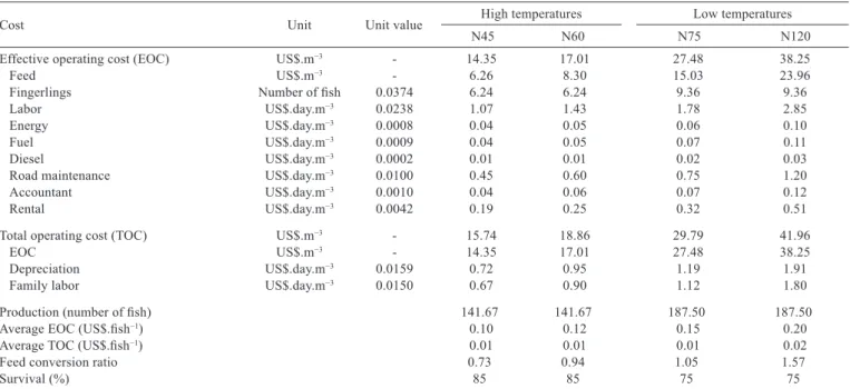
At the nursery stage, the fish were stocked with an average weight of 0.5 g and reared until 30 g (Table 1). Variations in the length of the cycles were verified (Figure 1) according to the stocking season and four distinct cycles were identified (45 and 60 days in high temperatures and 75 and 120 days in low temperatures). To compensate for lower performances during low-temperature periods, the fish farmer used higher densities (increasing from 167 fish.m−3
up to 250 fish.m−3). This method was insufficient to reduce
average costs because of the increase in the length of the cycle (Table 2). On the other hand, if the producer had chosen not to increase the stocking density, the production would have been smaller and the average cost would have increased. The feed was the most representative item on production cost (39.8 to 57.1%) depending on the cycle length. The acquisition of fingerlings was the second most representative cost, ranging from 22.3 to 39.6% (Table 2).
In the pre-finishing phase, the fish started with an average of 30 g and left the phase with 250 g. The length of the cycle varied from 60 to 120 days depending on the temperature. Considering the origin of these fish (nursery stage), however, there is a chance that the same product (250 g juvenile) can be produced with different costs as observed from four different cycles that resulted in distinct production costs, depending on the combination of its origin (nursery) and the cycle it would enter (Table 3). At this stage, regardless of the cycle length, an equal stocking density was used (200 fish.m−3).
To take extraneous variables into account as related to the TOC that may occur in 60 or 120 rearing days, the number of juveniles were increased and the participation of the feed was decreased. However, feed remained as the most representative item (49.6 to 69.4%), as the costs of the fry acquisition represented 22.1 to 46.0% (Table 3). Similar to the nursery stage, average costs increased with longer cycles.
Stage Crude protein (%) Weight (g) Pellet size (mm) DFF FR (%LW)
High temperatures Low temperatures
0.5 to 3.0 1 10 12 8
45 3.0 to 5.0 1.5 10 10 7
Nursery 5.0 to 10.0 1.7 10 10 7
40 10.0 to 30.0 2 10 9 6
Pre-finishing
32 30.0 to 250 4 to 6 3 6 to 4 4 to 3
Finishing 250 to 1000 6 to 8 3 4 to 1.5 3 to 1
Table 1 - Feeding management adopted for tilapia farming, according to weight and time of year
DFF - daily feeding frequency (meals day−1); FR - feeding rate in function of live weight (LW).
Cost Unit Unit value High temperatures Low temperatures
N45 N60 N75 N120
Effective operating cost (EOC) US$.m−3 - 14.35 17.01 27.48 38.25
Feed US$.m−3 - 6.26 8.30 15.03 23.96
Fingerlings Number of fish 0.0374 6.24 6.24 9.36 9.36
Labor US$.day.m−3 0.0238 1.07 1.43 1.78 2.85
Energy US$.day.m−3 0.0008 0.04 0.05 0.06 0.10
Fuel US$.day.m−3 0.0009 0.04 0.05 0.07 0.11
Diesel US$.day.m−3 0.0002 0.01 0.01 0.02 0.03
Road maintenance US$.day.m−3 0.0100 0.45 0.60 0.75 1.20
Accountant US$.day.m−3 0.0010 0.04 0.06 0.07 0.12
Rental US$.day.m−3 0.0042 0.19 0.25 0.32 0.51
Total operating cost (TOC) US$.m−3 - 15.74 18.86 29.79 41.96
EOC US$.m−3 - 14.35 17.01 27.48 38.25
Depreciation US$.day.m−3 0.0159 0.72 0.95 1.19 1.91
Family labor US$.day.m−3 0.0150 0.67 0.90 1.12 1.80
Production (number of fish) 141.67 141.67 187.50 187.50
Average EOC (US$.fish−1) 0.10 0.12 0.15 0.20
Average TOC (US$.fish−1) 0.01 0.01 0.01 0.02
Feed conversion ratio 0.73 0.94 1.05 1.57
Survival (%) 85 85 75 75
Table 2 - Total operating cost and productive performance obtained from different nursery production cycles in US$.m−3
To observe an average growth of 750 g (from 250 g to the final weight of 1000 g), production cycles lasted for 90 (high temperatures) or 150 days (low temperatures). Similar to the pre-finishing stage as related to the combination between the origin of the fish (pre-finishing possibilities) and the cycle it would enter (Figure 1), the final product (1000 g fish) may demonstrate up to eight different costs (Table 4). In both the nursery and the pre-finishing stages, the feed costs were the most representative in TOC (51.8 to 61.9%). The production cost of juveniles (250 g) was the second most representative item in TOC, representing 29.7 to 41.5%.
To compensate for lower performances during the low-temperature period in the nursery stage, the producer increased the stocking densities (Table 4). The average costs were increased, however, due to longer production cycles and even with greater production. Longer cycles (270 days) occurred when one of the three stages was performed in low temperatures, being amid higher average production costs. Among these, the ones with the lower average costs were the nursery phase at low temperatures, as well as the pre-finishing and finishing phases at high temperatures. Conversely, if such practice was adopted in the pre-finishing stage, the average cost of the fish would become the most representative variable among all studied cases.
The final product (1000 g tilapia) obtained in this study was destined for three distinct sales channels: 30%
to CEAGESP, 60% to processing, and 10% directly to the market. Depending on the destination of the product, an increased cost related to transport was added as US$0.007.kg−1
for the market, US$0.010.kg−1 for CEAGESP, or US$0.041.kg−1
for processing, which was included in the average TOC, since the quantity of fish transported is different (larger amounts require additional labor). To determine the average final cost, a weighted mean was obtained with trade costs in regard to the proportions of the product given to the destination, obtaining an average general cost (CEAGESP, processing, and market) from a sale of US$0.039.kg−1.
Gross income was constant when considering the cycles of 90 and 150 days separately. Profit was reduced with the increased production cycle and, consequently, the profitability index presented the same behavior, ranging from 16.58 to 26.26%. As sales prices were the same in all studied cases, the highest profitability rate was demonstrated for N45PF60T90, which means that all stages were performed in high temperatures. The longest cycles (270 days) occurred when one of the three stages was performed in low temperatures and were also among the lower profitability indices found.
Discussion
Tilapia farming in three distinct phases helped the producer to obtain better growth indices, shorter cycles, and greater control over production. At the end of each cycle,
Cost Unit Unit value PF60N45 PF60N60 PF60N75 PF60N120 PF120N45 PF120N60
Effective operating cost (EOC) US$.m−3 72.90 77.31 82.47 95.44 97.03 101.44
Feed US$.m−3 48.22 48.22 48.22 48.22 69.88 69.88
Juvenile I1 Number of fish 22.21 26.62 31.78 44.75 22.21 26.62
Labor US$.day.m−3 0.0238 1.43 1.43 1.43 1.43 2.85 2.85
Energy US$.m−3 0.05 0.05 0.05 0.05 0.10 0.10
Fuel US$.day.m−3 0.0008 0.05 0.05 0.05 0.05 0.11 0.11
Diesel US$.day.m−3 0.0009 0.01 0.01 0.01 0.01 0.03 0.03
Road maintenance US$.day.m−3 0.0100 0.60 0.60 0.60 0.60 1.20 1.20
Accountant US$.day.m−3 0.0010 0.06 0.06 0.06 0.06 0.12 0.12
Rental US$.day.m−3 0.0042 0.25 0.25 0.25 0.25 0.51 0.51
Total operating cost (TOC) US$.m−3 74.75 79.16 97.29 97.29 100.74 105.15
EOC US$.m−3 72.90 77.31 82.47 95.44 97.03 101.44
Depreciation US$.day.m−3 0.0159 0.95 0.95 0.95 0.95 1.91 1.91
Family labor US$.day.m−3 0.0150 0.90 0.90 0.90 0.90 1.80 1.80
Average EOC (US$.fish−1) 0.39 0.42 0.48 0.49 0.54 0.39
Average TOC (US$.fish−1) 0.40 0.43 0.49 0.51 0.56 0.40
Feed conversion ratio 1.16 1.18 1.20 1.26 1.56 1.59
Survival (%) 99 99 99 99 99 99
Table 3 - Total operating cost (TOC) and productive performance obtained from different cycles at pre-finishing in US$.m−3 for a production
of 200 fish.m−3
N - nursery (0.5 to 30 g); PF - pre-finishing (30 to 250 g); the number after stage identification represents total rearing time. Dollar exchange: US$1.00 = R$2.538.
the fish were separated by size to improve batch uniformity, which is highly desired among buyers. Carvalho et al. (2010) observed similar results such as a greater apparent feed conversion, daily average weight gain, and better homogeneity on farms where this sorting was performed. The same authors observed that fish presented almost twice the size reared without this separation. Nonetheless, Garcia et al. (2013) found that if fish are stocked at low densities at the beginning of the production cycle, sorting is not necessary and is discouraged due to high mortality rates shortly after handling, attributed to elevated stress.
The broad range of the cycle lengths relates to the time of the year and the water temperature, affirming the results found by Mainardes Pinto et al. (1989), who observed a one-month reduction in cycle length when starting during the spring (September) as compared with the fall (March). This is probably related to the effect of temperature on growth during the finishing stage, which is lower than initial stages. A decrease was observed in the growth performance for the animals during the winter, however, as reported by Scorvo Filho et al. (2008) and Graeff and Amaral Junior (2005). These authors recommended fish farmers to carry out the production cycles during spring and autumn (October to April), when the water temperatures are above 22 °C. Garcia et al. (2014) also reported greater
likelihood of disease during winter due to lower water renewal and higher organic matter accumulation, which may compromise production.
The practice of increasing densities to compensate low growth performances may not be the most appropriate strategy. Garcia et al. (2013) tested different stocking densities for tilapia and observed that higher densities lead to greater production costs and longer cycles, associated with low feed efficiency and limited growth due to tank volume. Garcia et al. (2014) found that fish subjected to high densities (before size separation and end of the cycle) present higher incidence of disease.
In general, there was an increase in production costs with size of the production cycle, which results from the use of production factors (e.g. land, capital, and labor) for longer periods and in higher volumes; thus, the extended stocking period is followed by an additional management cost both in fixed capital and fish. This corroborates with the results found by Garcia et al. (2013), who observed increased production costs along with the cycle length, due to lower growth rates in high densities. However, there is no clear trend of increasing the production cycle and increasing production costs, because in F90PF120N45 with a production cycle of 255 days, the average production cost (US$1.35 kg−1 ) was
higher than in F90PF60N120 (US$1.33 kg−1), which had a
Cost Unit Unit value PF60F90
N45
F90 PF60
N60
F90 PF60
N75
F90 PF60 N120
F90 PF120
N45
F90 PF120
N60
F150 PF60 N45
F150 PF60 N60 Effective operating cost (EOC) US$.m−3 116.47 118.70 121.30 127.85 129.59 134.79 165.58 168.47
Feed US$.m−3 71.28 71.28 71.28 71.28 71.28 71.28 105.48 105.48
Juvenile II1 number of fish 37.75 39.98 42.59 49.14 50.88 56.08 49.08 51.98
Labor US$.day.m−3 0.0238 2.14 2.14 2.14 2.14 2.14 2.14 3.57 3.57
Commercialization US$.m−3 3.75 3.75 3.75 3.75 3.75 3.75 4.87 4.87
Energy US$.day.m−3 0.0008 0.07 0.07 0.07 0.07 0.07 0.07 0.12 0.12
Fuel US$.day.m−3 0.0009 0.10 0.10 0.10 0.10 0.10 0.10 0.17 0.17
Road maintenance US$.day.m−3 0.0100 0.90 0.90 0.90 0.90 0.90 0.90 1.50 1.50
Accountant US$.day.m−3 0.0010 0.09 0.09 0.09 0.09 0.09 0.09 0.15 0.15
Rental US$.day.m−3 0.0042 0.38 0.38 0.38 0.38 0.38 0.38 0.64 0.64
Total operating cost (TOC) US$.m−3 119.25 121.47 124.08 130.63 132.37 137.57 170.21 173.10
EOC US$.m−3 116.47 118.70 121.30 127.85 129.59 134.79 165.58 168.47
Depreciation US$.day.m−3 0.0159 1.43 1.43 1.43 1.43 1.43 1.43 2.38 2.38
Family labor US$.day.m−3 0.0150 1.35 1.35 1.35 1.35 1.35 1.35 2.25 2.25
Average TOC (US$.kg−1) 1.22 1.24 1.27 1.33 1.35 1.40 1.34 1.36
Total production cycle (days) 195 210 225 270 255 270 255 270
Production (kg.m−3) 98.00 98.00 98.00 98.00 98.00 98.00 127.40 127.40
Revenue (US$.m−3) 166.42 166.42 166.42 166.42 166.42 166.42 216.35 216.35
Operating profit (US$.m−3) 43.41 41.19 38.58 32.03 30.29 25.09 41.24 38.35
Profitability index (%) 26.09 24.75 23.18 19.25 18.20 15.08 19.06 17.73
Feed conversion ratio 1.44 1.44 1.45 1.46 1.54 1.54 1.56 1.56
Survival (%) 98 98 98 98 98 98 98 98
Table 4 - Total operating cost, profitability indicators, and productive performance obtained from different cycles in the finishing stage
N - nursery (0.5 to 30 g); PF - pre-finishing (30 to 250 g); F - finishing (250 to 850 g); the number after stage identification represents total rearing time. Dollar exchange in US$1.00 = R$2.538.
production cycle of 270 days. The main factor to obtain higher production costs was the realization of the pre finishing in a low temperature.
Feed was the most expensive item in TOC, with increased importance during longer cycles; however, we must consider that growth and grow-out diet costs are embedded in the value of the juveniles (30 to 250 g) so that the share of this item is superior to these values when considering production as a whole (nursery, pre-finishing, and finishing). Marengoni (2008) noted that high feed supplies may lead to financial losses, especially when final biomass is low. Marques et al. (2003) reported that providing adequate quantities of feed reduce competition among fish, resulting in better batch uniformity and productive performance. The authors also observed that low efficiencies in the use of feeds and limited growth in high densities increase costs. Andrade et al. (2005) found a share of 52.3% of feed on total production cost. These authors also observed that feed price fluctuation, influenced by its input costs, makes it the most expensive item and drives variations in the production costs.
The present study identified more than one marketing channel, which gives the producers more flexibility on making decisions about the production and assuring the sale of the products, in which the processing industry is responsible for the purchase of 60% of the produced fish. Nevertheless, the security in selling production reduces the risk generated by the increased cost due to the low temperatures, resulting in a variation in profitability indices. Andrade et al. (2005) and Castellani and Barrela (2005) observed a variable profit driven by cost variation similar to what was observed in the present study, which showed a decreased profit and profitability index in longer cycles, demonstrating greater economic paybacks from lower production costs due to better production management. This is also corroborated by Garcia et al. (2013), who observed that shorter production cycles of fish reared in low densities received a 60% higher profit when compared with high densities.
Conclusions
The best production scenario is found when carrying out all of the rearing stages (nursery, pre-finishing and finishing) in high temperatures. Considering production as a whole, stocking fish in low temperatures demonstrates negative impacts on the total cycle length, increasing the production time by 38.46%. Even with longer cycles and greater production costs, no financial injury is found if one stage is performed in low temperatures, which allows the producer to offer the product regularly. In addition, a
greater flexibility exists in making management decisions of the production when associated to three marketing channels.
Acknowledgments
The authors acknowledge the financial support of the Conselho Nacional de Desenvolvimento Científico e Tecnológico (CNPq/140551/2013-1) and Agência Paulista de Tecnologia dos Agronegócios, Polo Regional Médio Paranapanema – Assis.
References
Andrade, R. L. B.; Wagner, R. L.; Mahl, I. and Martins, R. S. 2005. Custos de produção de tilápias (Oreochromis niloticus) em um modelo de propriedade da região oeste do Estado do Paraná, Brasil. Ciência Rural 35:198-203.
Bukenya, J. O. and Ssebisubi, M. 2014. Price integration in the farmed and wild fish markets in Uganda. Fisheries Science 80:1347-1358.
Carvalho, E. D.; Camargo, A. L. S. and Zanatta, A. S. 2010. Productive development of Nile tilapia raised in net cages at a public reservoir: brief analysis of the empirical model of classification. Ciência Rural 40:1616-1622.
Castellani, D. and Barrella, W. 2005. Caracterização da piscicultura na região do Vale da Ribeira - SP. Ciência e Agrotecnologia 29:168-176.
Garcia, F.; Romera, D. M. and Gozi, K. S. 2014. Enfermidades de tilápias do Nilo em tanques-rede. Pesquisa & Tecnologia 11. Garcia, F.; Romera, D. M.; Gozi, K. S.; Onaka, E. M.; Fonseca, F. S.;
Schalch, S. H. C.; Candeira, P. G.; Guerra, L. O. M.; Carmo, F. J.; Carneiro, D. J.; Martins, M. I. E. G. and Portella, M. C. 2013. Stocking density of Nile tilapia in cages placed in a hydroelectric reservoir. Aquaculture 410:51-56.
Graeff, A. and Amaral Junior, H. 2005. Engorda final de tilápias (Oreochromis niloticus) no meio-oeste catarinense no período de verão com alevinos nascidos no outono-inverno oriundos do litoral de Santa Catarina (Brasil). Archivos Latinoamericanos de Producción Animal 13:87-91.
IBGE - Instituto Brasileiro de Geografia e Estatística. 2014. Produção da Pecuária Municipal 2014. In: Ministério da Agricultura (ed.) No. 1., Rio de Janeiro.
Mainardes Pinto, C. S. R.; Verani, J. R.; Antoniutti, D. M. and Stempniewski, H. L. 1989. Estudo comparativo do crescimento de machos de Oreochromis niloticus em diferentes períodos de cultivo. Boletim do Instituto de Pesca 16:19-27.
Marengoni, N. G. 2008. Production of the Nile tilapia Oreochromis niloticus (Chitralada strain) reared in cages with different stocking densities. Archivos de Zootecnia 55:127-138.
Marques, N. R.; Hayashi, C.; Soares, C. M. and Soares, T. 2003. Níveis diários de arraçoamento para alevinos de tilápia do nilo (Oreochromis niloticus, L.) cultivados em baixas temperaturas. Semina: Ciências Biológicas e da Saúde 24:97-104.
Martins, C. V. B.; Oliveira, D. P.; Martins, R. S.; Hermes, C. A.; Oliveira, L. G.; Vaz, S. K.; Minozzo, M.G.; Cunha, M. and Zacarkina, C. E. 2001. Avaliação da piscicultura na região oeste do estado do Paraná. Boletim do Instituto de Pesca 27:77-84. Matsunaga, M.; Bemelmans, P. F.; Toledo, P. E. N.; Dulley, R. D.;
produção utilizado pelo IEA. Agricultura em São Paulo 23:123-139.
Nogueira A. C. and Rodrigues, T. 2007. Criação de tilápias em tanques-rede. Sebrae Bahia, Salvador.
Oliveira, E.; Santos, F. S.; Pereira, A. and Lima, C. 2007. Produção de tilápia: mercado, espécie, biologia e recria. Circular Técnica, 45. Embrapa Meio-Norte, Teresina.
Pereira, E. P. and Gameiro, A. H. 2007. Análise da tilapicultura brasileira com ênfase no comércio internacional. In: Congresso da Sociedade Brasileira de Economia, Administração e Sociologia Rural, Londrina. 14p.
Sabbag, O. J.; Rozales, R. R.; Tarsitano, M. A. A. and Silveira, A. N. 2007. Análise econômica da produção de tilápias (Oreochromis niloticus) em um modelo de propriedade associativista em Ilha Solteira/SP. Custos e @gronegócio on line 3:86-100.
Scorvo Filho, J. D.; Mainardes-Pinto, C. S. R.; Paiva, P. D.; Verani, J. R. and Silva, A. L. 2008. Custo operacional de produção da criação de tilápias tailandesas em tanques-rede, de pequeno volume, instalados em viveiros povoados e não povoados. Custos e @gronegócio on line 4:98-116.