A Reinforcement Learning Environment for Cooperative Multi-Agent Games: Enhancing Negotiation Skills

(1)

F

ACULDADE DE

E

NGENHARIA DA

U

NIVERSIDADE DO

P

ORTO

A Reinforcement Learning

Environment for Cooperative

Multi-Agent Games: Enhancing

Negotiation Skills

José Aleixo Peralta da Cruz

Mestrado Integrado em Engenharia Informática e Computação Supervisor: Prof. Henrique Lopes Cardoso

(2)

(3)

A Reinforcement Learning Environment for Cooperative

Multi-Agent Games: Enhancing Negotiation Skills

José Aleixo Peralta da Cruz

Mestrado Integrado em Engenharia Informática e Computação

Approved in oral examination by the committee:

Chair: Prof. Jorge Manuel Gomes Barbosa

External Examiner: Prof. Brígida Mónica Faria Supervisor: Prof. Henrique Lopes Cardoso

(4)

(5)

Abstract

In artificial intelligence, an agent is an autonomous program that interacts with its environment over time and decides its actions according to a given objective function. In a multi-agent system (MAS), multiple agents interact with each other. A MAS is decentralized, meaning that no agent controls other agents. Certain scenarios are inherently decentralized because the entities that in-habit it may need to act independently, with different or conflicting goals and information. Such situations can be naturally modeled as a MAS.

There are situations where an agent must cooperate with another agent in the same environ-ment to achieve its objective. However, there are cases where alternating between cooperative and adversarial behavior is the only way to achieve the final goal. Diplomacy is a multi-player board game, where the central aim of a player is to conquer Europe. To do so, a player must negotiate alliances and coordinate strategies with other players. The catch is that these agreements may either be public or private, and they are non-binding. No player has full information regarding its opponents’ intentions, and any player may break its established agreements. Creating a computer player (bot) capable of taking these factors into account is a difficult task because of the huge amount of possible plays and outcomes, and because it is challenging to measure the true strength of a player’s position.

The solution we propose is a custom Diplomacy environment that enables reinforcement learn-ing agents to submit agreements to other players. Agents can use this environment to learn how to negotiate using reinforcement learning methods. We created three different scenarios based on the same environment, which were designed to focus on different aspects of negotiation in Diplomacy. We tested each case with state-of-the-art reinforcement learning methods.

We analyzed the success of our approach by comparing agents trained in our environment with other bots built for the Diplomacy game. Because Diplomacy is a game heavily reliable on negotiation tactics, a bot that has a strong negotiation capability is more likely to win the game. However, there are few implemented Diplomacy bots that take advantage of being able to make agreements. From the existing bots, we compare our solution to bots that simplify the game’s rules by assuming that the deals made are binding, eliminating the problem of trust.

We found that while our environment is functional, and allows an agent to learn to act in Diplo-macy scenarios with a reduced scope of action, the learning process for more complex situations is extremely slow, even with an adjusted negotiation scope. Software and hardware limitations translate into a prohibitively long time for the training process in our environment, which allied to the extensive observation and action spaces results in an agent that is not proficient in playing Diplomacy. However, with the environment we developed, we hope to enable further research in this game and its particular challenges.

Continuing to tackle problems that have a social aspect using reinforcement learning tech-niques, and improving current solutions, could lead to systems capable of making better decisions in scenarios where negotiating and compromising is necessary. These systems could be used to

(6)

study situations with real-life applications in areas such as social science, politics, and economics, helping humans make better decisions in complicated conditions.

(7)

Resumo

Em inteligência artificial, um agente é um programa autónomo que interage com o ambiente ao longo do tempo e decide as suas ações de acordo com uma função objetivo. Num sistema multi-agente (SMA), vários multi-agentes interagem uns com os outros. Um SMA é descentralizado, isto é, nenhum agente controla os outros agentes. Certos cenários são inerentemente descentralizados porque as entidades que lhes pertencem agem de forma independente, com informação e objetivos diferentes ou conflituosos. Tais situações podem ser modeladas como um SMA.

Há situações em que um agente tem de cooperar com outro agente no mesmo ambiente para atingir a sua meta. No entanto, há casos onde alternar entre comportamento cooperativo e compet-itivo é a única forma de atingir o objetivo final. O Diplomacy é um jogo de tabuleiro multi-jogador, cujo principal objetivo é conquistar a Europa. Para tal, um jogador deve negociar alianças e co-ordenar estratégias com outros jogadores. A peculiaridade do jogo é que estes acordos podem ser públicos ou privados, e não-vinculativos. Nenhum jogador conhece as intenções do seu oponente e qualquer jogador pode quebrar qualquer acordo. Criar um jogador virtual (bot) capaz de ter em conta estes fatores é uma tarefa complexa, devido ao elevado número de jogadas e resultados possíveis, e porque é muito difícil um jogador avaliar a sua verdadeira posição e força no jogo.

A solução que propomos é um ambiente de Diplomacy personalizado, que permite que agentes que usem reinforcement learning possam submeter acordos aos outros jogadores. Criámos três cenários diferentes baseados no mesmo ambiente, que foram desenhados para se focarem em diferentes aspetos da negociação no Diplomacy. Testámos cada caso com métodos do estado da arte de reinforcement learning.

Analizámos o sucesso da nossa abordagem comparando os agentes treinados no nosso ambi-ente com outros bots construídos para o Diplomacy. Como o Diplomacy é um jogo que depende bastante da tática de negociação, um bot que saiba negociar bem tem mais hipóteses de ganhar o jogo. No entanto, há poucos bots de Diplomacy que tirem vantagem de poderem fazer acor-dos. Daqueles que existem, comparamos a nossa solução a bots que simplificam as regras do jogo, assumindo que os acordos feitos não podem ser quebrados, eliminando assim o problema da confiança.

Concluímos que apesar de o nosso ambiente ser funcional e permitir que um agente aprenda a agir em cenários do Diplomacy com um âmbito de ação reduzido, o processo de aprendizagem para situações mais complexas é extremamente lento, mesmo com um âmbito de negociação ajustado. Limitações de software e hardware traduzem-se num ciclo de aprendizagem muito demoroso, que aliado ao extenso espaço de observação e ação resulta num agente que não é proficiente no jogo de Diplomacy. Ainda assim, com o ambiente que desenvolvemos, esperamos facilitar pesquisas futuras sobre jogo e os seus desafios.

Continuar a resolver problemas que têm um aspeto social usando reinforcement learning e continuar a melhorar soluções atuais poderá levar a sistemas capazes de tomar melhores decisões em cenários onde negociação e compromisso sejam necessários. Estes sistemas podem ser usados

(8)

para estudar situações com aplicações na vida real, em áreas como a ciência social, a política e a economia, ajudando humanos a tomar melhores decisões em situações complicadas.

(9)

Acknowledgements

I would like to thank my supervisor Professor Henrique Lopes Cardoso for the guidance and support. I would also like to thank my family for always being encouraging and making it possible for me to do what I enjoy the most.

(10)

(11)

“A man provided with paper, pencil, and rubber, and subject to strict discipline, is in effect a universal machine.”

(12)

(13)

List of Figures

2.1 Agent-environment interface [SB18] . . . 6 2.2 Reinforcement learning with policy represented via a deep neural network [MAMK16]. 10 2.3 The actor-critic method architecture. [Yoo19] . . . 13 2.4 Comparison of several algorithms on different OpenAI Gym (Section3.2.3)

Mu-JoCo environments, training for one million time steps [SWD+17] (CEM stands for “cross-entropy method” [RK13]). . . 15 2.5 Interactions between agents in a multi-agent system. . . 15 2.6 Figure depicting a standard board for a Diplomacy game. The circles represent

supply centers. [Add01] . . . 17 3.1 Schematic illustration of the convolutional neural network used to learn to play

Atari games. . . 21 3.2 An example of the target map in Multiple Tank Defence. . . 23 5.1 Conceptual model of the Open AI Gym Diplomacy environment and agent. . . . 34 5.2 Sequential diagram of the Open AI Gym Diplomacy components, with the agent

as the actor. . . 38 6.1 Average rewards per episode (game) of an agent learning with ACKTR in the

negotiation environment from scratch (average of 3 executions over 46 episodes). The values have been smoothed using a window size of 3 episodes. Each game has a variable number of steps. A valid deal gives a positive reward+5, each invalid deal gives_−5. . . . 43 6.2 Rewards per episode (game) of an agent learning with PPO in scenario 2. The

values have been smoothed using a window size of 10 episodes. . . 46 6.3 Rewards per episode (game) of an agent learning with PPO in scenario 3. The

(16)

(17)

List of Tables

3.1 Feature comparison between the environments introduced in Sections3.2and3.3. 26 6.1 Victories and supply centers conquered by the the models trained in scenario 2

(forethought) and scenario 3 (no forethought) in 80 games played against six D-Brane bots with negotiation. . . 48 6.2 Number of games played as each power and average number of supply centers

(18)

(19)

Abbreviations

A2C Advantage Actor-Critic

A3C Asynchronous Advantage Actor-Critic

ACKTR Actor Critic using Kronecker-Factored Trust Region AI Artificial Intelligence

ANAC Automated Negotiating Agents Competition CNN Convolutional Neural Network

DRL Deep Reinforcement Learning MAS Multi-Agent System

MDP Markov Decision Process ML Machine Learning NN Neural Network

PPO Proximal Policy Optimization RL Reinforcement Learning RPC Remote Procedure Call

(20)

(21)

Chapter 1

Introduction

Artificial intelligence (AI) has become one of the most prominent fields of computer science dur-ing the past decade. The evolution of electronic components allowed computers to process vast amounts of information quickly and cheaply, which in turn revamped the interest of the commu-nity in machine learning (ML). The ability to learn from experience used to be associated uniquely with humans, however, modern software is also able to produce knowledge. Reinforcement learn-ing gives a software agent the capability of adaptation by trainlearn-ing. While computers are gettlearn-ing better at overcoming obstacles, they still have great difficulty with acting and adjusting to highly complex scenarios.

Humans live in society, meaning that we must often negotiate and cooperate with other people to achieve our goals. We make decisions on our daily interactions based on previous experience and intuition. For example, our trust in a person depends on past interactions and affects the way we communicate and act with that individual. AI is generally employed to help humans make decisions regarding a particular problem. However, current AI programs are not capable of deciding on socially complicated scenarios, where negotiation and cooperation are very intricate, as well as humans.

Games have always been an essential test-bed for AI research. There has been extensive re-search aimed mostly at adversarial games. However, games where negotiation and cooperation are encouraged or necessary have not been the target of such a thorough investigation. Experimenting with this type of games is important because they mimic the actual interactions that occur in a society. Negotiating, reaching an agreement and deciding whether or not to respect that agreement is all part of a person’s daily life.

The work presented in this document focuses on the cooperation aspects of games. Instead of taking strategy into account, we will try to improve a software agent’s performance on a decision-making scenario by negotiating with other agents.

In the remaining of this chapter, we expose the motivations, objectives, and structure of this dissertation.

(22)

Introduction

1.1 Motivation

Stochastic scenarios are everywhere in the natural world. Decision-making in these circumstances is not as straightforward as in deterministic situations. Even humans struggle to make choices when faced with uncertainty. Game theory models have come to facilitate this task, allowing one solution or strategy to be used for multiple problems of the same type. These models arise from tests conducted across a diversity of games.

Researchers have focused mostly on adversarial games with one opponent, such as Chess [Dro93] and Go [SHM+16]. However, in many real-life situations, different entities can be cooperative, instead of strictly competitive. Such scenarios can be naturally modeled using a multi-agent sys-tem (MAS), where independent entities interact with each other. To address this type of situations, some attention has slowly shifted to cooperative games ([NNN18] and [Ope18]). In cooperative games, different players cooperate with each other to surpass a certain obstacle or reach a deter-mined goal. Still, few MAS-related works include the social aspect of cooperation.

Diplomacy [Cal00] is a board game which is incredibly complex. It involves adversarial as well as cooperative decisions. Players can communicate with each other and reach agreements or create alliances. But the deals they make are not binding and the players may betray allies. The social aspect of Diplomacy makes it a perfect test-bed for cooperation strategies in adversarial environments.

Because the search-tree of Diplomacy is very large, achieving the best performance in the game using a deterministic method is very complicated. Instead, we will explore the usage of reinforcement learning methods, which have been very successful in making an agent learn to play a game. However, the time and storage requirements of tabular methods are prohibitive. As such, approximate RL methods must be employed.

1.2 Objectives

The objective of this work is to design and implement an architecture for a single agent capable of learning how to incorporate social aspects on its decision-making process. This capability is crucial to winning a game of Diplomacy. This aspiration encompasses smaller goals, such as modeling a reinforcement learning approach to cooperative negotiation games, implementing the model and then training it.

In the end, we will evaluate the model in experimental scenarios and try to answer the follow-ing research questions:

1. How to create an environment with negotiation for reinforcement learning agents?

2. Is a reinforcement learning model appropriate for negotiation scenarios with a large search space?

3. How should a reinforcement learning model be structured to learn how to negotiate in games with cooperation and competition?

(23)

Introduction

With the answers to these questions, we wish to understand if a program could adapt itself to both known and unknown situations where social aspects influence the final outcome. Associat-ing cooperative and adversarial tactics is extremely useful in numerous real-world game theory scenarios, such as in politics and economics.

1.3 Document Structure

The current document comprises six more chapters. In Chapter2, we provide an overview of es-sential concepts related to machine learning and reinforcement learning, as well as state-of-the-art deep reinforcement learning techniques, to provide background for what we mention in the sub-sequent chapters. We also give information about multi-agent systems and negotiation games and introduce the game of Diplomacy. Chapter3 exhibits relevant work in reinforcement learning, current environments aimed at testing deep reinforcement learning methods and negotiation tech-niques, and the analysis of the gap between the scope of the current work and other approaches. Chapter4contains the framing of Diplomacy in game theory and the formalization of the problem we propose to solve. Specifically, we formalize negotiation in Diplomacy as a Markov decision process. Chapter5 addresses the implementation of our proposal, namely the system structure, the tools utilized, and the implementation details. Chapter6 includes the details about the per-formed experiments, respective results, and discussion. Chapter7presents the conclusions of the current project, which include an overview of all the work done, the answers to our initial research questions, and eventual improvements to our solution.

(24)

(25)

Chapter 2

Background

In this chapter we present an overview of concepts that provide the basis for the rest of the doc-ument. We will include notions related to machine learning, reinforcement learning and deep reinforcement learning. These notions are essential to understanding how and why approaches differ from one to another. We base ourselves in established definitions and current literature and try to present all terms with a consistent interpretation. In particular, we gather information from a survey by Li [Li17] and a book by Sutton [SB18] and complement it with papers about the latest state of the art.

2.1 Machine Learning

Machine learning is the study of computer algorithms that learn from data and improve their performance in making predictions and decisions. It is a subarea of artificial intelligence. Its prin-ciples are based on probability theory, statistics, and optimization. A machine learning algorithm has an input data-set, a loss function, and a model. The input data-set contains the information that the model should use to generate its output. The loss function is the penalty for a bad output. The model tries to compute a result to get the lowest loss possible. In mathematical terms, it tries to minimize the loss function. This process of optimization is called learning or training.

There are three big branches of machine learning: supervised learning, unsupervised learning and reinforcement learning. In supervised learning, the input data is labeled, which means that an example - a particular piece of data - contains the values of the features and of one or more labels. A feature is an independent variable and a label is a dependent variable whose value is influenced by a set of features. A supervised learning model tries to predict the label value from the given set of feature values. Because the training data-set is labeled, the feedback is explicit, that is, the model knows whether it got the output correctly or not by comparing it to the values of the labels. In unsupervised learning, the input data contains features but is not labeled. No feedback is given, so the model tries to find patterns in the data on its own. In reinforcement learning, there

(26)

Background

Figure 2.1: Agent-environment interface [SB18]

is evaluative, not explicit, feedback. The feedback tells the model how well it is doing, but not if it has actually done its task properly or not. It is important to understand that reinforcement learning is not a subset of unsupervised learning as there is feedback. It is not supervised learning either because the feedback is not explicit.

2.2 Reinforcement Learning

An intelligent agent is a program that perceives the environment through sensors and acts upon it using actuators. In reinforcement learning, an agent interacts with its surroundings over time, which we call the environment. At each time step t, the agent perceives a set of environmental conditions, which make up a state st, and selects an action at to take. Depending on the resulting

state st+1, the agent gets a reward rt+1. This interaction is illustrated in Figure2.1.

For instance, if an agent is learning how to drive a car according to traffic laws, the reward it receives should depend on whether or not it obeys the law. If it accelerates when the traffic light is red, it should get a low reward. If it stops on red lights, it should get a high reward. Eventually, the agent will learn that the best thing to do is stopping on red lights, which is how you respect the law. The objective of a reinforcement learning agent is to maximize the reward functionR. Previously, we referred that a machine learning algorithm has a loss or cost function that it should minimize. In RL, the cost function is the inverse ofR.

According to Sutton [SB18], reinforcement learning algorithms have the following elements: • a policy π, which defines the learning agent’s way of behaving at a given time;

• a reward function R, which defines the goal of a reinforcement learning problem;

• a value function V , which defines the amount of reward an agent may accumulate over time from a given state.

If the transitions of the environment are known, there may be an additional element that is the model of the environment, which is used to plan actions, by predicting their consequences before actually committing to them.

(27)

Background

To better understand each element, we should formalize a reinforcement learning problem. We can describe one as a Markov Decision Process (MDP), where:

• S is a finite set of states; • A is a finite set of actions;

• Pa(st, st+1) is the probability that an action a on state st at a given time t will lead to state

st+1at time t+ 1;

• Ra(st, st+1) is the immediate reward rt+1 of transitioning from state st to state st+1 after

taking action a.

In a MDP, the probability of each possible value for st+1 and rt+1 depends only on the

im-mediately preceding state and action - it does not depend on the history of previous states and actions. Because of this, a state in a MDP must include all information about the past inter-actions that makes a difference in future decisions. In mathematical terms, this translates to P(st+1|st) = P(st+1|s1, s2, ..., st). A state st that obeys this constraint possesses the Markov

prop-erty. Pa(st, st+1) is the transition function, which represents the environment’s dynamics. If the

transition function is well defined, we may create a model of the environment. Model-based rein-forcement learning methods simulate interactions with the environment using the created model, as opposed to model-free methods that learn by interacting directly with the environment. For the remaining of this document, we will only be considering model-free methods, as most studied scenarios are too complex to be adequately used with model-based approaches.

A policy is a probability distribution that defines the likelihood of an agent choosing a certain action given the state of the environment. In a MDP, a policy is a mapping from S to probabilities of selecting each element of A. If an agent is following a policy π at time step t, then π(a_{|s) is the} probability of at = a if st = s. For example, a greedy policy would make the agent always choose

the action that gives the best reward. That is, if a is the action that leads to the highest reward in state s, then π(a_{|s) = 1, while all other actions would have an associated probability equal to 0.} However, this would mean that no action besides the best one was tried by the agent. Executing an action with the best immediate reward may not lead to the best total reward, meaning the agent would get stuck in a local minimum. Effectively, one of the greatest challenges in reinforcement learning is maintaining a balance between exploitation and exploration.

Exploitinginvolves using what an agent already knows to make a decision. Exploring involves learning new things. A simple example of a policy that allows an agent to explore is the ε-greedy policy, where the agent chooses greedily most of the time but, with probability ε, it selects among all the actions with equal likelihood. This allows the agent to explore new options and get closer to the global optimum solution.

The reward function defines the values of the rewards for each possible transition in a MDP, that is, the values of Ra(st, st+1) for every a∈ A and (st, st+1)∈ S × S. A reinforcement learning

agent will maximize the reward function by selecting the set of actions that triggers the transitions that provide the highest combined reward.

(28)

Background

The value function is an element that helps the agent to achieve the best global solution, by allowing it to estimate how promising a certain state (or a state-action pair) is. For instance, an agent may choose an action with lower immediate reward in favor for a state that is more promising, so that it receives more reward in the long-run. At a certain time step t, we can define the expected return or expected reward of a state, denoted Gt, as Equation2.1,

Gt =. T

∑

k=t+1

γk−t−1Rk (2.1)

where γ is a discount factor with value equal or less than 1. The number of time steps T is set depending on whether the task is episodic or continuous. In an episodic task, the number of time steps T is finite and all future rewards may or may not have the same weight in the final result. In a continuous task, the number of time steps is infinite, therefore, in order to avoid an infinite sum and ensure convergence, the condition γ< 1 has to be true.

The value function of a state s under a policy π, denoted vπ(s), can then be defined as the

expected return when starting in s and following π (Equation2.2).

vπ(s) . = Eπ[Gt | St= s] = Eπ[ ∞

∑

k=0 γkRt+k+1| St = s], for all s∈ S (2.2)

The vπ function is the state-value function for policy π. From Equation 2.2, we may define

the value of taking action a in state s under a policy π as the expected return when starting from s, taking the action a and from that time forward following policy π as Equation2.3.

qπ(s, a) . = Eπ[Gt| St = s, At= a] = Eπ[ ∞

∑

k=0 γkRt+k+1| St = s, At = t] (2.3)

The qπ function is the action-value function for policy π. We can also write the state-value

function in terms of the action-value function, as shown in Equation 2.4, which is the weighted sum of the action-value for every action a available in state s, where the weight is the probability of the action a being chosen according to policy π.

v_π(s) =

_∑

a

π(a_|s)qπ(s, a) (2.4)

However, the agent does not know the true values of either of these two functions. If it did, the problem would be easily solvable. So the agent estimates these values.

One of the most common methods for estimating action-value, which is often called the Q-value, is doing the average of n observed rewards for a given action a in a state s (Equation2.5). With each new observation, a new value must be stored in memory, representing the reward of taking the action on a given time step.

Qn=.

R₁+ R2+ ... + Rn−1

(29)

Background

The memory requirements grow linearly with this method of value update. However, there is another way of calculating the average keeping the memory requirements constant, described in Equation2.6. This update rule is the basis of most reinforcement learning methods. The general form is described in Equation2.7.

Qn+1=. 1 n n

∑

i=1 Ri= Qn+ 1 n[Rn− Qn] (2.6)

NewEstimate_{← OldEstimate + StepSize[Target − OldEstimate]} (2.7) The expression[Target− OldEstimate] is an error or loss in the estimate. It is reduced by taking a step toward the target. The target is presumed to indicate a desirable direction in which to "move", though it may be noisy. Therefore the main objective of a RL algorithm is to reduce the difference between the old estimates and the target value, until the current estimate converges. The StepSize parameter determines how much weight the newly found information has on the old value update. The impact of the target value shows how important it is to define a suitable reward function for a problem.

2.2.1 Q-Learning

Q-learning [WD92] is a tabular solution reinforcement learning method. In tabular solution meth-ods, the state and action spaces are small enough for the value functions to be represented as arrays or tables. In Q-learning, the value function takes a pair state-action and is updated with the rule in Equation2.8.

Q(St, At)← Q(St, At) + α[Rt+1+ γ max

a [Q(St+1, a)]− Q(St, At)] (2.8)

Q-learning is called an off-policy method because it does not follow the current policy π to choose the action a from the next state St+1 in order to update the current state value. Instead,

it chooses the greedy (i.e. max reward) action for the update (maxa[Q(St+1, a)]). In other words,

Q-learning assumes that it is always following a greedy policy when it updates its estimates, even if the current policy π is not greedy. An advantage of this separation is that the estimation policy, used to update Q-values, is independent of the behaviour policy, used to choose which states and actions should be updated. It has been proven that Q-learning, provided infinite computation time and a partly-random policy, can always identify an optimal policy for a finite Markov decision process [Mel01].

However, in problems where the search space is too large, tabular methods such as Q-Learning are not appropriate, because of hardware limitations and costs. Instead, we choose to use approx-imate solution methods. In these methods, the agent makes decisions on states it has not seen before based on previous encounters with different states. The key issue becomes generalization. Neural networks are models capable of doing good function approximations and helping on the

(30)

Background

task of generalization. This naturally led to the use of deep learning to regress functions for use in reinforcement learning agents, which is called deep reinforcement learning.

2.3 Deep Reinforcement Learning

In deep reinforcement learning (DRL), deep neural networks are used to approximate the value function or find the optimal policy. In tabular methods, all values in tables are stored in memory. However, large search trees make storing and evaluating all these values unfeasible. By using a neural network, we can avoid the space and time problem, and calculate values for new and unfamiliar states. Neural networks are used as a function approximator, vastly reducing memory requirements, as shown in Figure2.2. Most DRL techniques are relatively recent, since they are enabled by the vast power of modern computer processors.

Figure 2.2: Reinforcement learning with policy represented via a deep neural net-work [MAMK16].

2.3.1 Value-Based Methods

Value-based deep reinforcement learning methods use a value network. A value network is a neural network that assigns a value to every state s of the environment by calculating the expected cumulative reward for that state. Every state the agent observes goes through the value network. The states which lead to higher rewards obviously get higher values in the network. Instead of states, the network may assign scores to state-action pairs (s, a), which is the case of the Deep Q-Network.

2.3.1.1 Deep Q-Network

The Deep Q-Network (DQN) method [MKS+13] is a deep reinforcement model that uses a variant of Q-learning. While the traditional Q-learning method requires storing the value function Q for each state-action pair, the DQN approximates Q(s, a). In this approach, the Q-value function is generalized, instead of “remembered” by the agent.

(31)

Background

Using a deep neural network allows generalization, but carries some challenges. If we take the target[Rt+1+ γ maxa[Q(St+1, a)] of the Q-learning method, we observe that it depends on Q itself.

When a function approximator such as a neural network is used to represent Q, the target may become unstable, which provokes the neural network to diverge or never stabilize. This instability is due to a couple of causes: the possible correlations in sequential observations and the correlation between action-values and target values.

When employing neural networks, it is important to make sure that samples are independent of each other and follow similar data distributions. To address this, instead of feeding the DQN with a mini-batch of sequential observations, such as the last 100 observations, a mechanism called experience replay is used. To perform experience replay, we store a considerable number of observations in a buffer and, instead of feeding them sequentially to the neural network, we extract a mini-batch randomly. This reduces the correlation between observations, because we are using both recent as well as old observations, so they are more independent of each other and the agent doesn’t “forget” what it had previously learned.

Because the Q-function is updated with values of itself, changing a Q-value for a single state-action pair also alters the value for other pairs. This leads to a moving target that the neural network keeps chasing, never converging. The solution applied by DQN is to create two neural networks: a Q-network, with a parameter vector θ , and a target-network, with a parameter vector (θ−). The Q-network is updated as it would normally be, while the target-network is only updated and synchronized periodically with the Q-network. To calculate the target we use the more stable value of the target-network, therefore the target will be less correlated with the Q-value. The loss function for the update rule on time step t effectively becomes what is described in Equation2.9, which is the function the neural network tries to minimize.

Li(θi) = E(s,a,r,s0₎[(r + γ max

a [Q(s 0_{, a, θ}−

t )]− Q(s,a,θt))2] (2.9) 2.3.2 Policy Gradient Methods

In policy gradient or policy-based methods a policy depends on a vector of parameters θ , in contrast to value-based methods such as DQN, which depend on value functions. In a policy-based method, the policy is defined as π(a_{|s,θ), expressing that choosing an action a depends not} only on the current state s, but also on the values of the θ vector. To determine how good a policy with parameters θ is, we use a performance measure, which is a function J(θ ) that takes these parameters and determines their benefit. The learning process tries to maximize the performance measure, which means the updates made to the values of the parameters approximate gradient ascent in J (Equation2.10).

θt+1= θt+ α \∆J(θt) (2.10)

The performance measure is calculated differently for episodic and continuous cases. For the sake of relevancy, we will only refer to the episodic cases performance. In these cases, the

(32)

Background

performance measure is the expected reward of following the policy π with parameters θ starting on the initial state s0(Equation2.11).

J(θ )= v. πθ(s0) . =

_∑

a

πθ(a|s0)qπθ(s0, a) (2.11) The gradient of the performance measure is then calculated as shown in Equation 2.12, ac-cording to the Policy Gradient theorem, where µπθ(s) is the probability of being at state s when following policy πθ and ∝ means proportional to.

∇θJ(θ ) = ∇θvπθ(s0) ∝

∑

s_∈S µπθ(s)

∑

a_∈A q_π_θ(s, a)∇θπθ(a|s) =

_∑

s_∈S µπθ(s)

∑

a_∈A πθ(a|s)qπθπ(s, a) ∇θπθ(a|s) πθ(a|s) = Eπθ[qπθ(s, a)∇θln πθ(a|s)] (2.12)

A policy’s parameters can be chosen arbitrarily, as long as π(a_{|s,θ) is differentiable with} respect to its parameters. One common way of defining θ is as the vector of all the weights of a deep neural network that tries to choose the best action for a given state. Then, a numerical preference h(s, a, θ ) is associated to each state-action pair. Actions with higher h value have higher probabilities of being selected.

One of the advantages of policy-based methods over value-based methods is that the policy may be a simpler function to approximate than the value function. For extensive spaces, the number of state-action values to learn can be quite large. Policy-based methods avoid this because they only need to learn a number of parameters that is far less than the space count. Another advantage is that policy-based methods can learn stochastic policies, while action-value methods have no natural way of finding stochastic policies, as they converge to a deterministic policy. In scenarios that require selecting actions with arbitrary probabilities, a stochastic policy leads to the best outcome. For instance, when playing a game of Rock-Paper-Scissors against an opponent, having a deterministic policy allows the adversary to counter every move we do. Hence, the best solution is to select an action with a certain probability.

A major problem with the “vanilla” policy gradient loss referred in Equation2.12is that the diversity of the set of states visited in an episode (also called trajectory), can result in a high discrepancy between the cumulative reward values of different episodes. Consequently, gener-ated gradients are too noisy and the variance is too high. One way of reducing the variance and increasing learning stability is to subtract the cumulative reward by a baseline b(st).

For example, let’s say the values of ∇θln πθ(a|s) are [0.5,0.3,0.2] and the values of qπθ(s, a) are [1000, 1001, 1002] for three different trajectories. The variance of the product of the values (which originates from Equation2.12) is equal to Var(0.5_{∗1000,0.3∗1001,0.2∗1002) = 232700.} By using a simple constant baseline b(st) = 1000, the variance then becomes Var(0.5∗ 0,0.3 ∗

(33)

Background

2.3.2.1 Advantage Actor-Critic (A2C)

Some methods explore the incorporation of a baseline in order to stabilize gradients and accelerate learning. Actor-critic methods are policy-based methods that also learn to approximate a value function. These are considered hybrid methods, as they combine approaches used in value-based methods and policy-based methods. The purpose of learning the value function is precisely to use it as a baseline during the learning process and assist on the policy update.

An actor-critic method has a learning model split in two components, depicted in Figure2.3. One component, labeled the actor, determines the action to take on a given state. The actor is a reference to the learned policy, which dictates how the agent acts. The other component is called the critic and evaluates the impact of that action, which is a reference to the value function. TD error (temporal-difference error) is the difference between the estimates of a value at different time steps (Equation 2.7). The actor will update its values, and therefore the choices it makes, according to the TD-error calculated by the critic. The critic will also make adjustments to its values based on the TD-error.

Figure 2.3: The actor-critic method architecture. [Yoo19]

Another common baseline to use when learning a policy is the advantage of taking an action aon a state s, given by A(s, a) = Q(s, a)_{−V (s). The advantage function captures how good an} action is compared to other actions that may be taken in the same state.

The Advantage Actor-Critic (A2C) [WML+17] method combines both notions in its name. In A2C, the critic learns the advantage function, instead of the Q-values, thus reducing the high

(34)

Background

variance of policy networks and stabilizing the model. It is based on the Asynchronous Advan-tage Actor-Critic (A3C) [MBM+16]. In A3C, different workers run parallel environments and asynchronously update a global network. However, experimental results determined that there was no gain with the asynchronous feature of A3C and removing it simplified implementations, resulting in the A2C.

An algorithm that improves on the concept of A2C is the Actor Critic using Kronecker-factored Trust Region (ACKTR) [WML+17]. ACKTR uses distributed Kronecker factoriza-tion [MG15] to optimize the calculation of the gradient update. This update can be 25% more expensive than A2C, but it leads to better results.

2.3.2.2 Proximal Policy Optimization (PPO)

Policy-gradient methods are generally too sensitive to the choice of the StepSize parameter (Equa-tion2.7). If the steps are too small, the learning progression is extremely slow. If the steps are too large, the model may overshoot an optimal region and end up with a noisy learning signal.

The Trust Region Policy Optimization (TRPO) [SLM+15] tries to fix this issue by setting a constraint (Equation2.13) on how much a new policy can differ from the old one, using the Kull-back–Leibler divergence (KL) [KL51], which measures the difference between two probability distributions. maximize θ E t[ πθ(at|st) πθold(at|st) A(st, at)] subject to Et[KL[πθold(·|st), πθ(·|st)]]≤ δ (2.13)

With this constraint, the policy is kept in a trust region, so that it avoids taking larger steps than recommended.

The Proximal Policy Optimization (PPO) [SWD+17] improves on TRPO by embedding the constraint on the objective function. This facilitates and speeds up calculations while maintain-ing the policy in a trust region. Let rt(θ ) denote the probability ratio rt(θ ) = _ππθ(at|st)

θold(at|st), so that rt(θold) = 1 and ε is a hyper-parameter. Then the objective function of PPO is given by

Equa-tion2.14.

maximize

θ E

t[min(rt(θ )A(st, at), clip(rt(θ ), 1− ε,1 + ε)A(st, at)] (2.14)

The first term of the objective function is the objective function of TRPO. The second term clips the ratio between the old and new probability distributions of the policy, removing the incen-tive for changing the policy beyond[1_{− ε,1 + ε]. The minimum term is used so the final objective} is a lower (pessimistic) bound of the unclipped objective. The performance improvement of PPO over A2C and TRPO for the same environments can be visualized in Figure2.4.

(35)

Background 0 1000000 500 0 500 1000 1500 2000 HalfCheetah-v1 0 1000000 0 500 1000 1500 2000 2500 Hopper-v1 0 1000000 0 2000 4000 6000 8000 InvertedDoublePendulum-v1 0 1000000 0 200 400 600 800 1000 InvertedPendulum-v1 0 1000000 120 100 80 60 40 20 Reacher-v1 0 1000000 0 20 40 60 80 100 120 Swimmer-v1 0 1000000 0 1000 2000 3000 Walker2d-v1 A2C

A2C + Trust Region CEM PPO (Clip) Vanilla PG, Adaptive TRPO

Figure 2.4: Comparison of several algorithms on different OpenAI Gym (Section3.2.3) MuJoCo environments, training for one million time steps [SWD+17] (CEM stands for “cross-entropy method” [RK13]).

2.4 Multi-Agent Systems and Negotiation Games

In a multi-agent system, two or more agents exist and interact in the environment (Figure 2.5). Each agent is autonomous in their decision making and independent from the others. The system is decentralized because no agent determines the decisions of other agents. If the agents are not in the same physical location, but still share information by communicating with each other, then the system is also distributed. Some scenarios are inherently decentralized and may be naturally modeled as a multi-agent system. For example, if different people or organizations have different goals and conflicting information, a MAS is useful to manage their interactions [SV00]. Some other problems have characteristics that are solved more easily with a multi-agent system model. A task that may be divided into independent sub-tasks that can be handled by different agents could benefit from the parallelism that a MAS provides as a distributed system.

(36)

Background

Games have always been a target of research to experiment problem-solving methods that could be applied in real-life scenarios. However, most research has been aimed towards adversarial games. According to Nash [Nas51], non-cooperative (or competitive) games involve competition with individual opponents, where alliances may be created but are only self-enforced. This means that there is no external authority obliging players to maintain their agreements. The alliance is kept while the players deem it convenient. By contrast, cooperative games have coalitions (groups of individual players) competing against each other. These coalitions are enforced by a third party, effectively prohibiting players from breaking an arrangement.

If there is no communication between players, then the coalitions are formed due to Nash equilibrium [N+50] or to explicit action constraints [GGR88], in competitive and cooperative scenarios, respectively. In a Nash equilibrium, if players have nothing to gain by competing against each other, they will form a self-enforced coalition. With constraints, a player is bound not take any action that may harm other players. However, if there is communication between players, then they may coordinate with each other to reach agreements, whether they are binding (cooperative games) or not (non-cooperative games). Games with communication may be modeled under game theory as bargaining or negotiation games [OR94].

Negotiation serves as a conflict solver between entities. For instance, people negotiate between themselves to achieve an agreement. Whether it is setting the time for a meeting or purchasing a house, negotiation is much present in the real-word. In a multi-agent system, each agent has its own set of goals and utility functions. Sometimes, it is beneficial for agents to cooperate with each other, but issues or conflicts may arise. Therefore agents also need to negotiate with each other. We will use negotiation games to test the efficacy of deep reinforcement learning in negotiation, more specifically a game called Diplomacy.

2.4.1 Diplomacy: the Game

Diplomacy [Cal00] is a board game with 20th century Europe as a setting. The game is best played by seven players. Each player represents one of the seven great powers: England, France, Austria, Germany, Italy, Turkey, and Russia. The objective of a great power (or country) is to conquer Europe.

A Diplomacy board (Figure2.6) has 34 provinces. There are three types of provinces: inland, water and coastal. Some provinces have a supply center. Each great power possesses two types of units: armies and fleets. Only armies move on inland provinces and only fleets move on water provinces. Both types of units may occupy a coastal province.

At the start of a game, each power controls three supply centers, with the exception of Russia, which controls four. The remaining 12 supply centers are not occupied at the start of the game. The number of units a power controls at the beginning of the game is the same as the number of supply centers it owns.

In Diplomacy, a turn represents six months of time. The first turn is called the Spring turn and the next the Fall turn. In each turn, players may give units orders to hold (stay in the same province), move (attack adjacent provinces) or support (support the orders of units from the same

(37)

Background

Figure 2.6: Figure depicting a standard board for a Diplomacy game. The circles represent supply centers. [Add01]

or other players). Because all units have the same strength, the only way to win conflicts (standoffs) is to support other units’ orders. Each supporting unit adds one unit of strength to the order it is supporting.

The characteristic that makes Diplomacy appropriate for the study of cooperation and nego-tiation is the Diplomatic Phase that occurs at the beginning of every turn. In this phase, players meet together one-to-one or in small groups. They may create alliances publicly or secretly and coordinate unit orders with each other. However, the agreements that the players make are not binding. A player may disrespect an understanding or an alliance. To survive, a player needs to cooperate with others. To win, a player must eventually stand alone.

After the Diplomatic Phase, the players write down the orders they will give to each of their units. The plans are all revealed at once and are not reversible. The conflicts that emerge from the orders given are solved and the players settle the ownership of the provinces according to the conflicts’ outcomes. A power gains or loses units in accordance with the number of supply centers it controls. If one power controls 18 or more supply centers at the end of a Fall turn, that player is declared the winner and the game ends.

(38)

(39)

Chapter 3

Related Work

In this chapter, we provide an overview of relevant breakthroughs in reinforcement learning, the current state of the art of deep reinforcement learning applied to games, and related work regarding negotiation in Diplomacy. We also evaluate the gap between the scope of the current project and other endeavors.

3.1 Reinforcement Learning Applied to Games

Donald Michie created one of the first systems to use reinforcement learning in 1961 [Mic61]. It consisted of a set of simple matchboxes that allowed an operator to play Tic-Tac-Toe (Noughts and Crosses) against a human. Michie eventually developed his idea by modeling problems into sub-games and solving them with a program called BOXES [MC68] which was capable of balancing a simulated pole in a cart. BOXES obtained knowledge through trial and error. Each "box" would contain information about what action to take and how many times it worked well towards the final objective, considering the actions taken before-hand.

In 1992, Christopher Watkins formalized the Q-Learning technique (presented in Section2.2.1). The introduction of the off-policy Q-value function vastly improved the practicability and feasibil-ity of reinforcement learning and boosted its interest in the scientific communfeasibil-ity.

A few years later, Gerald Tesauro created a neural network capable of learning how to play backgammon by playing against itself [Tes94]. The network, called TD-Gammon, achieved a staggering level of performance by closely matching world-class human players. It also surpassed the performance of a previous supervised learning approach of Tesauro [Tes89], trained with the data of actual human games, revealing the great potential behind reinforcement learning.

In 2013, DeepMind researchers combined deep neural networks with reinforcement learning to play more than one game of Atari, using only the frames of the game as an input (see Sec-tion3.2.1). It was one of the first works using neural networks to approximate value functions for reinforcement learning and of generalizing the representation of the environment enough for the

(40)

Related Work

agent to learn multiple games. DeepMind’s research boosted the interest in deep reinforcement learning, showing that agents can learn how to execute complex tasks with performance equal or higher than humans.

3.2 Deep Reinforcement Learning Environments

Much of the recent research accomplished in deep reinforcement learning involves creating or mimicking an environment and then applying novel methods to solve the problem imposed by that environment. In this section, we explore some modern DRL research environments applied to games.

3.2.1 Atari Games

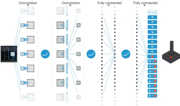
One meaningful challenge that deep reinforcement learning agents face is coming up with a mean-ingful representation of the input information they receive. The difficulty of this challenge in-creases with the dimension of the state representation. A video game, for instance, is constantly transmitting complex information to a human player. Mnih et al. [MKS+13,MKS+15] approached this challenge by creating an agent capable of playing Atari games, having the frames of the game as the only state representation. The frame’s pixels are pre-processed and then fed to a Deep Q-Network with experience replay (see Section2.3.1.1). The first layers of the DQN network are convolutional while the remaining are fully connected (Figure3.1). For a frame of input, the neu-ral network outputs the Q-values for the different actions that can be taken on that state. These actions map to the same controls a human has when playing the game. This approach achieved super-human performance in several Atari games, revealing the power of convolutional neural networks to generate representations of a complex environment.

3.2.2 Go

In 2016, DeepMind researchers created AlphaGo [SHM+16], a program capable of playing the Go board game. Go is a game of perfect information. However, the number of different sequences of moves is approximately 250150, which makes exhaustive tree search infeasible. AlphaGo became a landmark when it defeated the number one ranked player in the world in a series of Go games.

AlphaGo uses convolution neural networks (CNN) to construct a representation of the game environment from the image of the board, similarly to the approach to Atari games (described in Section3.2.1). This representation is passed to neural networks which reduce the breadth and depth of the action search tree. The depth of the search tree is reduced by replacing the sub-tree of each state s by its predicted value (which the probability of winning the game from that state), using an approximate value function v(s). The breadth of the search is diminished by sampling the actions from a policy π(s, a), which results in only considering a small set of actions rather than all possible actions. The neural network that approximates the value function is the value network and the neural network that determines the policy is the policy network. The policy

(41)

Related Work

Figure 3.1: Schematic illustration of the convolutional neural network used to learn to play Atari games.

network is initially trained using supervised learning, with data from samples of games between Go professionals. After the initial training, the policy network is trained through policy gradient reinforcement learning.

The policy is improved through self-play. A modified Monte Carlo method called Monte Carlo Tree Search (MCTS) algorithm is implemented to take into account the policy values and explores moves with a lookahead search, expanding the most promising states and eventually selecting what considers to be the best move.

An improved version of AlphaGo called AlphaGo Zero [SSS+17] learned how to play Go without any human input or feedback. While the original AlphaGo was trained using data from ac-tual human games, AlphaGo Zero learned how to play from scratch and only from playing against itself. AlphaGo Zero’s performance surpassed the original program’s, becoming the world’s best Go player in just 40 days [SH17].

3.2.3 OpenAI Gym

OpenAI Gym [BCP+16] is a Python toolkit for executing reinforcement learning agents that op-erate on given environments. The great advantage that Gym carries is that it defines an interface to which all the agents and environments must obey. Therefore, the implementation of an agent is independent of the environment and vice-versa. An agent just needs little (if any) adaptation to act on different environment, as the uniform interface will make sure the structure of the informa-tion the agent receives is almost the same for each environment. This consistency promotes the

(42)

Related Work

performance comparison of one agent in different conditions, and of different agents in the same conditions. Two of the methods defined by the Gym interface are:

• reset: A function that resets the environment to a new initial state and returns its initial observation. It is used to initiate a new episode after the previous is done.

• step: A function that receives an action as an argument and returns the consequent obser-vation(the state of the environment) and reward (the value of the state-action pair), whether the episode has ended (done) and additional information that the environment can provide (info).

Each environment must also define the following fields:

• action space: The object that sets the space used to generate an action.

• observation space: The object that sets the space used to generate the state of the environment.

• reward range: A tuple used to set the minimum and maximum possible rewards for a step. Default is[_−∞,∞].

This specification represents an abstraction that encompasses most reinforcement learning problems. Given that RL algorithms are very general and can be applied to a multitude of sit-uations, being able to reuse a solution in different scenarios is very beneficial, as it adds to its usefulness. While Gym is directed to reinforcement learning, since it is built on Python, it is eas-ier to connect existing Python machine learning libraries with Gym agents and make use of the deep reinforcement learning techniques that those frameworks provide.

3.2.4 Multiple Tank Defence

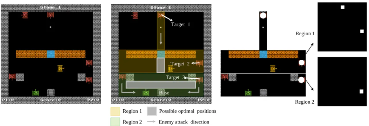
Multiple Tank Defence is a custom multi-agent environment where either one or two tanks must defend their base together from enemy tanks. The defending tanks must avoid getting hit by the enemies while eliminating them. The terrain of the game is customizable, which ensures that the agents will be challenged with new environment conditions.

Each agent receives a reward of 10 for killing an enemy tank. The necessity for such a simple reward function comes from the fact that agents become easily suck in local minimum solutions due to insufficient exploration in environment with sparse rewards. However, when training with-out human guidance, the tanks acquired an attacking stance, where they would try to kill as many enemy tanks as possible. To solve this problem, the agents were each given a target map. This map details which sections of the environment a tank can “see” (Figure3.2). Therefore, it defines the area of action of each agent. The target maps are defined by a human, but have led the agents to take a more defensive and cooperative stance to defend the base. This indicates that providing human strategies leads agents to easily attain an expected solution in a short training time, without needing human feedback during that phase.

(43)

Related Work

Region 1 Region 2

Possible optimal positions Enemy attack direction

Region 1 Region 2 Target 1 Target 2 Target 3 Base

Figure 3.2: An example of the target map in Multiple Tank Defence.

3.2.5 OpenAI Five

Dota 2 is a real time multiplayer strategy game, consisting of two teams of five players. To win, a team must destroy the enemy’s base. OpenAI have developed a team of neural networks called OpenAI Five [Ope18] to tackle the problem that Dota 2 presents. The tremendous complexity of Dota 2 poses great challenges to an AI. These challenges include: its long time horizon, where most actions have minor impact individually but others affect the game strategically, with conse-quences that can play out over an entire game; its partially-observed state as each team only knows what is around each player and base; and its high-dimensional observation and action space (up to 170,000 possible actions per player in a given time step).

OpenAI Five uses a dedicated system to run PPO (an algorithm described in Section2.3.2.2) with an immense computational power. Several copies of the game are created with independent agents. The agents then sync their experience to a common optimizer. This results in a system capable of learning 900 years-worth of experience in a single day. OpenAI Five improved its performance over the course of two years, starting by beating individual players and eventually dethroning the world-champions of Dota 2. It demonstrated the strength of PPO and parallel learning.

3.3 Multi-Agent Negotiation Environments

Many real-life scenarios can be modeled as games where players benefit from communicating and compromising. One of the challenges of negotiation is determining the utility value of an agreement when it is not explicitly given or when the environment has complex rules. De Jonge & Zhang [DJZ17] developed an adapted Monte Carlo Tree Search agent to calculate the utility value of a negotiation in a perfect information game. Having full information about the opponents negotiations, the agent was able to accurately determine the opponent’s utility function. However, realistically not all information is known when negotiating.

(44)

Related Work

3.3.1 Diplomacy Environments

Diplomacy encompasses the challenge of negotiating without knowing the true strength of either player’s position, as agreements are made in private. The challenge that Diplomacy poses is an intriguing test for software agents. Some environments have been developed to facilitate the implementation of computer Diplomacy players. In this section, we expose some of them.

DAIDE[RNW07] (Diplomacy Artificial Intelligence Development Environment) is a frame-work that defines a communication model, protocol, and syntax for an environment where mul-tiple Diplomacy agents can compete with each other. The suggested model is a client-server design, where each Diplomacy player and observer are clients that connect to a single server over an IP network. This server handles all game logic. Each player is an independent process, that may communicate with other players through the game server. Parlance [RNW09] is a platform-independent Python application that follows the DAIDE specification. It materializes the game server, allowing clients to connect through sockets. Once a player connects to the server, it re-mains connected during the whole game, listening to the messages the server sends about the state of the game. Upon handling such communications, it decides whether or not it should send information back to the server, depending on the type of message.

DipGame[FSN] is a Java framework for developing bots (computer players) for DAIDE-based servers, such as Parlance. It includes a game manager, which allows to easily select which players should participate in a game and observe the output of a game in real time. It also includes a negotiation server, separate from the game server, which mediates all negotiation between players, obeying to the DAIDE syntax.

BANDANA [JS17] is an extension of DipGame, with a simplified negotiation server and lan-guage. It facilitates the creation of bots, control of game settings, and analysis of logs and re-sults and it is implemented in Java. The Diplomacy league of the Automated Negotiating Agents Competition (ANAC) [dJBA+19] asks for participants to conceive their submissions using the BANDANA framework.

Two types of Diplomacy players can be created using BANDANA – a player that only makes tactical decisions or a player that also negotiates with its opponents. Tactical choices concern the orders to be given to each unit controlled by the player. Negotiations involve making agreements with other players about future tactical decisions. In the original Diplomacy game, these nego-tiations are non-binding, meaning that a player may not respect a deal it has previously reached. However, in BANDANA deals are binding: a player may not disobey an agreement it has estab-lished during the game. The removal of the trust issue that non-binding agreements bear simplifies the action space of mediation. Tactical orders and negotiations are handled by two different mod-ules in a BANDANA player. They may communicate with each other, but that is not mandatory. A complete BANDANA player consists of these two modules, that should obey to a defined inter-face.

(45)

Related Work

3.3.2 Negotiating Diplomacy Bots

The current work is inspired by previous endeavors to create an AI that can master the Diplomacy game. While none used approximate reinforcement learning methods, each approach showed a distinct negotiation procedure.

Webb et al. [WCW+08] used the DAIDE environment to develop the Diplominator. The Diplominator has a custom tactical and negotiation module. At the beginning of the game, the bot tries to propose peace to all other players. Being in peace means that the Diplominator will be less probable to attack units of the power that makes part of the agreement. However, if the allied power is hindering the conquest of a supply center, it is treated as an enemy. If an allied power starts getting too strong, the Diplominator will “back-stab” it. The moment for the back-stab is decided according to how many supply centers it stands to gain by attacking the ally at a given time. If the Diplominator is put in a less favorable position after the back-stab, it will give up on it and re-request friendship.

Ferreira et al. [FLCR15] created a Diplomacy bot called DipBlue using the DipGame frame-work. DipBlue utilizes a trust ratio to adjust the likelihood of opponents fulfilling agreements. It changes the trust ratio according to the actions taken by opponents, such as attacks or betrayals. It then combines this trust ratio with a value for opponent strength. DipBlue tries to create alliances with the stronger players and attack the weaker ones, with the objective of surviving as long as possible.

Marinheiro and Lopes Cardoso [MLC17] suggested a generic architecture called Alpha for agents that act on games with a mix of cooperation and competition, including Diplomacy. Alpha contains different modules with different functions. They communicate between themselves, ana-lyzing the various aspects of the game. For instance, the Foreign Office is the module responsible for negotiating and the Intelligence Office is in charge of predicting opponents moves. While each agent has its own individual goal, cooperating with other players is encouraged as it results in a better outcome for each actor. Some of the challenges noted are related to accurately evaluating moves and player positions, given the social context of the game. Also, the possibility of betrayals due to non-binding agreement adds a new problem related to trust.

In the 2018 edition of the Automated Negotiating Agents Competition (ANAC), four bots applied for the Diplomacy competition [dJBA+19]. However, there was no winner because no bot was capable of passing the minimum requisites to triumph. The competition was divided into two rounds with the objective of testing both strategies for deal proposal and deal acceptance. The two most notorious submissions to the competition were the bots named CoalitionBot and Gunma. CoalitionBot’s play-style is described as passive. It proposes deals to achieve peace and it always accepts incoming deals. Because of this, it is exposed to the opponents’ strategies and it does not exploit the weaknesses of adversaries. Gunma, on the other hand, is a greedy player. It only proposes deals that would benefit itself and does not take into consideration its allies. However, it is less selfish when accepting deals, given that it will accept deals that do not cause it to lose anything, even if it gains nothing from it.

(46)

Related Work

3.4 Gap Analysis

The environments presented in this chapter focus on different challenges. Therefore, the features that each one of them offers are distinct, as shown in Table3.1.

Table 3.1: Feature comparison between the environments introduced in Sections3.2and3.3. Environment DRL Multi-Agent Negotiation

Atari X

Go X

OpenAI Gym X

Multiple Tank Defence X X

OpenAI Five X X

BANDANA X X

On the one hand, negotiation in a multi-agent system is relatively unexplored in current RL works. On the other hand, recent Diplomacy negotiation bots do not employ any RL mechanism, and the available environments do not enable easy integration with deep reinforcement learning frameworks in particular. With the current work, we are attempting to model an approach that uti-lizes deep reinforcement learning to play cooperative negotiation games, using Diplomacy as our testbed. More specifically, we intend to contribute to the scientific community by creating an envi-ronment that allows the study of negotiation strategies in a multi-agent system using reinforcement learning techniques.

(47)

Chapter 4

Negotiation in Diplomacy

This chapter contains the details and formalization of the problem we are trying to solve according to the notions given in Chapter2. More specifically, we frame Diplomacy (Section2.4.1) in game theory and explain how it serves as a test-bed for our approach. Furthermore, we formalize it as a Markov Decision Process (MDP) and expose our assumptions and constraints.

4.1 Diplomacy in Game Theory

We can classify Diplomacy under game theory [OR94]. It belongs to the following types:

• deterministic. No game event is random. Every outcome depends only on the actions taken by the players, therefore for a given state, the same set of actions will always lead to the same result.

• non-cooperative. There is no external authority to enforce cooperation. Players will only cooperate while it benefits them.

• symmetric. The payoffs for playing a particular strategy depend only on the other strategies employed, not on who is executing them. For example, no player loses by gaining control of a supply center. The objective is the same for every player.

• zero-sum. For a player to win control over a supply center another one has to lose it. How-ever, if we only consider a subset of players, such as two allies, there are some situations that can be considered non-zero-sum. For example, when an alliance conquers supply centers, the aggregate gain for the players in that alliance is superior to zero. Still, for a subset of players to win, another subset of players must lose. Therefore the scenario which includes all players is zero-sum.

• simultaneous. The orders of the players are all revealed at the same time, so no player can take advantage from knowing what the other players will do.

A Reinforcement Learning Environment for Cooperative Multi-Agent Games: Enhancing Negotiation Skills

F

E

U

P

A Reinforcement Learning

Environment for Cooperative

Multi-Agent Games: Enhancing

Negotiation Skills

José Aleixo Peralta da Cruz

A Reinforcement Learning Environment for Cooperative

Multi-Agent Games: Enhancing Negotiation Skills

José Aleixo Peralta da Cruz

Mestrado Integrado em Engenharia Informática e Computação

Approved in oral examination by the committee:

Abstract

Resumo

Acknowledgements

Contents

List of Figures

List of Tables

Abbreviations

Chapter 1

Introduction

1.1

Motivation

1.2

Objectives

1.3

Document Structure

Chapter 2

Background

2.1

Machine Learning

2.2

Reinforcement Learning

∑

∑

∑

∑

∑

2.3

Deep Reinforcement Learning

∑

∑

∑

∑

∑

2.4

Multi-Agent Systems and Negotiation Games

Chapter 3

Related Work

3.1

Reinforcement Learning Applied to Games

3.2

Deep Reinforcement Learning Environments

3.3

Multi-Agent Negotiation Environments

3.4

Gap Analysis

Chapter 4

Negotiation in Diplomacy

4.1

Diplomacy in Game Theory

_∑

_∑

_∑