Dynamic programming for aligning sketch maps

i

Dynamic Programming for

Aligning Sketch Maps

Dissertation submitted in partial fulfillment of the requirements for the Degree of Master of Science in Geospatial Technologies

February 24, 2020

_______________________________________

Violeta Ana Luz Sosa León

vsosaleo@uni-muenster.com https://github.com/violetasdev

Supervised by:

Prof. Dr. Angela Schwering Institute for Geoinformatics

University of Münster

Co-supervised by:

Dr. Malumbo Chipofya Institute for Geoinformatics

University of Münster

and

Prof. Dr. Marco Painho

Nova Information Management School Universidade Nova de Lisboa __________________________________

ii

Declaration of Academic Integrity

I hereby confirm that this thesis on Dynamic Programming for Aligning Sketch Maps is solely my own work and that I have used no sources or aids other than the ones stated. All passages in my thesis for which other sources, including electronic media, have been used, be it direct quotes or content references, have been acknowledged as such and the sources cited.

February 24, 2020

___________________________________

I agree to have my thesis checked in order to rule out potential similarities with other works and to have my thesis stored in a database for this purpose.

February 24, 2020

iii

Acknowledgments

I am grateful to the joint program coordinated by Dr. Christoph Brox at the University of Muenster, Prof. Dr. Joaquín Huerta at Jaume I University, and my also supervisor, Prof. Dr. Marco Painho at the University Nova de Lisboa for this opportunity to have one of the most significant experiences in my academic, social, and professional aspects. I hope you can continue helping more students in the future with the program from which I have been part.

A special thanks to my supervisors, Prof. Dr. Angela Schwering and Dr. Malumbo Chipofya, from whom I have learned in a range of different topics from theoretical to technical, in how to engage research and to manage myself to improve continually. Your kind support and knowledge have made possible this thesis to flourish and be an essential step in my future academic and professional life. I am inspired and motivated to be more involved in the Spatial Intelligence research field and continuing exploring the interdisciplinarity approaches between spatial cognition and computer science.

Finally, I would like to acknowledge my family, professors, and friends in Mexico, Colombia, and Japan, and my new friends all over the world. Thanks for your overwhelming care and support in this adventure, pushing me out of my comfort zone to learn from every experience and giving me love, courage, and advice when I most needed it.

iv

TABLE OF CONTENTS

Chapter 1 INTRODUCTION ... 1.2 1.1 Related work and motivation... 1.2 1.2 Research questions and objectives ... 1.3 1.3 General methodology ... 1.4 1.4 Thesis outline ... 1.5 Chapter 2 BACKGROUND ... 2.6 2.1 Sketch Maps ... 2.6 2.2 The graph matching problem ... 2.7 2.3 Qualitative Spatial Representation ... 2.9 2.3.1 Qualitative Spatial Calculi ... 2.10 2.3.2 Qualitative Constraint Networks ... 2.11 2.3.3 Local Compatibility Matrix ... 2.12 2.4 Link analysis ... 2.13 2.5 Reinforcement Learning Algorithms ... 2.13 Chapter 3 METHODOLOGY ... 3.16 3.1 Implementation workflow ... 3.16 3.2 System setup ... 3.18 3.2.1 Python ... 3.18 3.2.2 SmartSkeMa framework ... 3.19 3.2.3 Metric map generation ... 3.21 3.2.4 Execution environment ... 3.21 3.3 Input Datasets ... 3.21 3.3.1 Artificial dataset ... 3.23 3.3.2 El Remanso... 3.23 3.3.3 Mailua Ranch ... 3.25

v 3.4 Qualitative Analysis ... 3.26 3.5 Score system... 3.27 3.5.1 Page Rank ... 3.27 3.5.2 Spectral Solution Technique ... 3.30 3.5.3 Heuristic scores from LCM ... 3.31 3.6 Searching Algorithms ... 3.33 3.6.1 Tabu Search ... 3.33 3.6.2 SARSA ... 3.37 3.7 Evaluation ... 3.41 Chapter 4 RESULTS AND DISCUSSION ... 4.43 4.1 Performance ... 4.46 4.1.1 Execution time ... 4.46 4.1.2 Precision and Recall ... 4.48 4.2 Alignment Results... 4.51 4.3 Discussion ... 4.53 4.4 Limitations ... 4.56 Chapter 5 CONCLUSIONS ... 5.58 5.1 Future Work ... 5.60 Chapter 6 REFERENCES ... 6.61

vi

List of Tables

Table 1 Spatial Calculi for Qualitative Representations ... 2.10 Table 2 SmartSkeMa feature types ... 3.22 Table 3 Artificial dataset features ... 3.23 Table 4 El Remanso dataset features ... 3.25 Table 5 Mailua Ranch dataset features ... 3.26 Table 6 Confusion Matrix ... 3.41 Table 7 Mailua Ranch Marsh feature attributes ... 4.44 Table 8 Link Analysis sample results ... 4.45 Table 9 LCM(H1) score sample ... 4.46 Table 10 Artificial SVG: Precision and Recall Results ... 4.49 Table 11 El Remanso: Precision and Recall Results (H2) ... 4.49 Table 12 El Remanso: Precision and Recall Results (H1) ... 4.50 Table 13 Mailua Ranch: Precision and recall results ... 4.50 Table 14 Artificial SVG: Alignment result sample ... 4.51 Table 15 El Remanso: alignment result sample ... 4.52 Table 16 Mailua Ranch: alignment result sample ... 4.52

vii

List of Figures

Figure 1 Thesis challenges outline ... 1.4 Figure 2 Methodology overview ... 1.5 Figure 3 Graph: nodes, edges, and labels (M. Chipofya et al., 2017) .. 2.8 Figure 4 Graph Matching techniques (Conte et al., 2016) ... 2.8 Figure 5 Graph labels and nodes (color) (M. Chipofya et al., 2017) . 2.12 Figure 6 Framework implementation workflow ... 3.17 Figure 7 Thesis implementation workflow ... 3.18 Figure 8 SmartSkeMa interface ... 3.19 Figure 9 SmartSkeMa vectorization ... 3.20 Figure 10 SmartSkeMa Geometry Editor user interface ... 3.20 Figure 11 Artificial dataset SVG ... 3.23 Figure 12 El Remanso neighborhood (Google Maps view) ... 3.24 Figure 13 El Remanso: sketch (left) and metric (right) maps ... 3.24 Figure 14 Mailua Ranch: sketch (left) and metric (right) maps ... 3.25 Figure 15 Transition probabilities for a graph G (Ceri et al., 2013) .. 3.28 Figure 16 Link Analysis evaluation diagram ... 3.29 Figure 17 Diagram for the Spectral Solution Technique algorithm .. 3.31 Figure 18 Heuristic scores calculation workflow ... 3.33 Figure 19 Tabu Search workflow diagram ... 3.34 Figure 20 SARSA dynamic ... 3.37 Figure 21 Mailua Ranch vectorized sketch map ... 4.43 Figure 22 Qualitative representation input maps ... 4.44

viii Figure 23 Artificial SVG execution time ... 4.47 Figure 24 El Remanso execution time ... 4.47 Figure 25 Mailua ranch execution time ... 4.48 Figure 26 Tabu clustering alignment ... 4.54 Figure 27 SARSA(H2) clustering alignment ... 4.55 Figure 28 SARSA(H2) compared to SARSA(H1) alignment ... 4.55

ix

List of Algorithms

Algorithm 1. Tabu Search ... 3.35

Algorithm 2 SARSA Main ... 3.40

x

List of Acronyms

DPSM Dynamic Programming Sketch Maps Implementation

FP False Positive

FN False Negative

GIS Geographic Information System

LA Link Analysis

LCM Local Compatibility Matrix

LCM(H1) First heuristic score from the LCM

LCM(H2) Second heuristic score from the LCM

QMC Qualitative Constraint Map

QCN Qualitative Constraint Network

SST Spectral Solution Technique

TP True Positive

1.1

Abstract

Sketch maps play an important role in communicating spatial knowledge, particularly in applications interested in identifying correspondences to metric maps for land tenure in rural communities. The interpretation of a sketch map is linked to the users’ spatial reasoning and the number of features included. Additionally, in order to make use of the information provided by sketch maps, the integration with information systems is needed but is convoluted. The process of identifying which element in the base map is being represented in the sketch map involves the use of correct descriptors and structures to manage them. In the past years, different methods to give a solution to the sketch matching problem employs iterative methods using static scores to create a subset of correspondences. In this thesis, we propose an implementation for the automatic aligning of the sketch to metric maps, based on dynamic programming techniques from reinforcement learning. Our solution is distinctive from other approaches as it searches for pair equivalences by exploring the environment of the search space and learning from positive rewards derived from a custom scoring system. Scores are used to evaluate the likeliness of a candidate pair to belong to the final solution, and the results are back up in a state-value function to recover the best subset states and recovering the highest scored combinations. Reinforcement learning algorithms are dynamic and robust solutions for finding the best solution in an ample search space. The proposed workflow improves the outcoming spatial configuration for the aligned features compared to previous approaches, specifically the Tabu Search.

Keywords: sketch map, metric map, dynamic programming, tabu search, learning algorithm, link analysis, alignment.

1.2

CHAPTER 1 INTRODUCTION

1.1 RELATED WORK AND MOTIVATION

As humans, we communicate our perception of the elements surrounding us by using different tools: book descriptions, paintings, and more elaborated representations like maps in different types, including sketch maps. Sketch maps contain a set of items displaying the author’s conception of the space, providing spatial information useful for studying and understanding the environment in which she lives (Malumbo Chipofya, Wang, & Schwering, 2011). To be able to unveil the meaning behind a sketch map without the author’s feedback, it is necessary to compare every structure to a more structured representation of geographical elements, such as metric maps (Klaus Broelemann, Jiang, & Schwering, 2016). By having them side-by-side, it is possible to identify the abstraction created in the sketched map and relate it to a specific item in the metric map. As the elements increase in the input map, the association’s complexity with the metric map also grows, and therefore the relationships included, requiring automatizing the aligning process.

The difficulties in this task include the definition of appropriate representations of the problem space in order to structure the search for correspondences (Wallgrün, Wolter, & Richter, 2010). Graphs are robust information structures with gained popularity to represent formal structures for displaying relations of different types such as spatial, geometrical, or conceptual (Bunke, 2000). They are often used to examine the relationships correspondence and consistency of the data structure implemented with an exhaustive analysis of their distribution defined as a case of graph matching problems, with different approaches according to the category in which the graph representation belongs (Foggia, Percannella, & Vento, 2014). Diverse techniques to solve the matching problem include the measure of distances, composite graph similarities, string-based methods, and statistical graph matching (Emmert-Streib, Dehmer, & Shi, 2016). One of the current implementations for the sketch to the metric alignment problem, translated as a graph matching problem with the implementation of Qualitative Constraint

1.3 Networks, analyzes specialized local structures to evaluate candidate pairs while searching for correspondences (Malumbo Chipofya, Schwering, & Binor, 2013). The correspondence problem using LCM has arisen solutions with exponential time complexity, which may not be a feasible solution for significant scale problems (Malumbo Chipofya, 2018). In the recent years, the artificial intelligence field has developed different techniques for giving solutions to large scale tasks involved with graph nature problems in computer vision, integrating algorithms that rely on patterns and deductions from the accessible information (Foggia et al., 2014). By exploiting the capabilities of Local Compatibility Matrices, newer algorithms for significant scale problems, and other similarities measures studied for matching tasks in other fields, how to improve the pair selection process by taking advantage of past exploration in local compatibility matrices?

1.2 RESEARCH QUESTIONS AND OBJECTIVES

This research aims to implement and compare two searching algorithms to identify the next optimal pair selection during the matching process between a sketch and a metric map.The following research questions are defined:

• How can the pair selection algorithm be modified to increase the number of correctly matching objects for alignment between sketch and metric maps? • How can the exploration in the pair selection algorithm be used to recover

critical information for the matching process between sketch and metric maps? • Does the new pair selection algorithm improve the alignment solution?

In order to answer the previous research questions, the following objectives are defined:

• Calculate a new selection score system for the matching process

• Retain feedback for future decision processes during the exploration in the search algorithm

• Evaluate the matching results comparing the search algorithms implemented to measure changes in performance

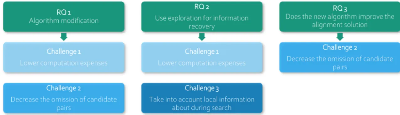
1.4 The open challenges identified from the sketch to metric map alignment process are addressed with the stated research questions as displayed in Figure 1:

1.3 GENERAL METHODOLOGY

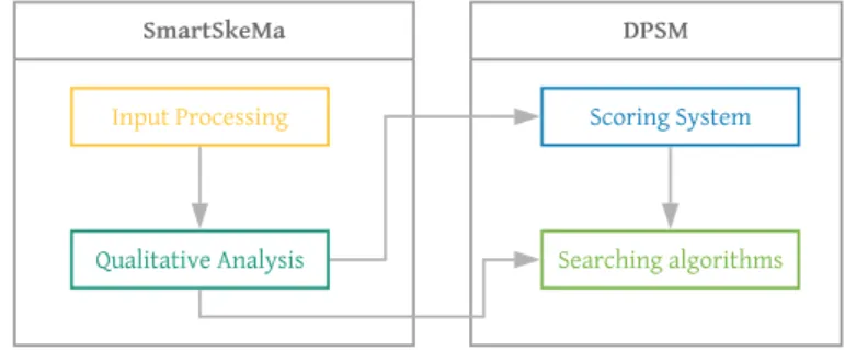
The sketch to metric map alignment process workflow is divided into 5 modules: first of all, for the Input Processing, the sketch and metric map are processed in the SmartSkeMa framework to translate the features from geometries to a set of vectors by a computer vision segmentation process and then identify the spatial relationships from the vectorized features are organized in a graph like data structure, implementing Qualitative Constraint Networks. Secondly, the Qualitative Analysis module analyzes the output from the framework and assesses the compatibility of each feature in terms of feature type and similarity. The next step in the workflow is the Score System, which provides the measurements of Link Analysis ranking score, Spectral Solution clustering solution, and the two Local Compatibility Matrices Heuristic Scores H1 and H2 to evaluate the likeliness of a candidate pair to belong to the alignment solution. Finally, in the Searching Algorithms component, we implement two different algorithms to find correspondences between candidate pairs: a metaheuristic approach named the Tabu Search and a reinforcement learning algorithm, SARSA. We compare the provided solutions in terms of their performance, precision, and recall. Figure 2 summarizes the processes outlined and their outputs.

RQ 1 Algorithm modification

Challenge 1 Lower computation expenses

Challenge 2

Decrease the omission of candidate pairs

RQ 2

Use exploration for information recovery

Challenge 1 Lower computation expenses

Challenge 3

Take into account local information about during search

RQ 3

Does the new algorithm improve the alignment solution

Challenge 2

Decrease the omission of candidate pairs

1.5

Figure 2 Methodology overview

1.4 THESIS OUTLINE

The following sections are organized as follows:

• Chapter 2 describes the theoretical background introducing the concepts employed in this thesis including the use of sketch maps, the importance and past work for giving solution to the graph matching problem, the spatial representation calculus and data structures implemented to make use of them, and finally, a review to different strategies for searching algorithms.

• In Chapter 3, the proposed methodology is outlined in detail, describing the sketch and metric maps used as an input and the assessment of the compatibility between features followed by the definition of the scoring system for the pair selection, and finally, the design and pseudo code for the Tabu and SARSA algorithms.

• Chapter 4 displays the results of the workflow described in Chapter 3 to automatically align sketch maps followed by the evaluation process to measure the performance and quality of the solution in terms of precision and recall for each search algorithm, discussion of the results, as well as the findings and the encountered limitations.

2.6

CHAPTER 2 BACKGROUND

This section presents an outline of the concepts supporting this thesis from the literature. Initially, we present Sketch Maps and a brief background to the graph matching problem, introducing qualitative spatial representations and the different qualitative calculi involved. Secondly, we outline the theory of Link Analysis to identify the importance of vicinities in local exploration, and finally, we portray strategies to solve searching problems from the perspective of artificial intelligence.

2.1 SKETCH MAPS

Sketch maps are representations of the space surrounding an individual decomposed into different spatial elements such as roads, buildings, and other physical features describing the relationships between the scene elements (Schwering & Wang, 2010). Moreover, every individual due to different experiences give an interpretation of the objects and their relationships being a topic of interest in research for map sketching in schools, governmental projects, and academia.

The decoding of the information from a sketch (input) map to a metric (output) map is an approach by projects such as the SmartSkeMa framework delivering the scene spatial segmentation, qualitative representations, and input/output alignment process (Schwering et al., 2014). Along with the implementation, several analyses and techniques have been implemented to give solutions to the alignment process resulting in theoretical implications and findings such as Qualitative Constraint Matrices. On the other hand, the its4land project is one of the real-world applications of this kind of framework. By using sketch maps, communities in Kenya are able to participate in land delimitation and appropriation, helping to the management of natural and human-build resources.

To accurate relate subjective maps and metric maps, techniques for assessing qualitative map alignment has been applied to find matches among the input representation such as a sketched entity, and one or several entities in a metric map using Local Compatibility Matrices (LCM) (M. C. Chipofya,

2.7 Schultz, & Schwering, 2016). The version of the implemented Tabu algorithm aims to face challenges such as the omission of promissory matching candidates and long execution times on large datasets. However, the dynamic metaheuristics generated in Chipofya’s algorithm gave better performance and accuracy versus standard compatibility matrices; leaving open the research for the refinement during the iterative match-candidates selection process since it rapidly leaves the matching process without candidates due to the removal of not compatible local pairs at a particular stage. As the search space grows, it may be helpful to identify how to associate potential additions during the exploration in previous regions of the search space (Malumbo Chipofya et al., 2013)

2.2 THE GRAPH MATCHING PROBLEM

The most significant benefit of graphs is that they can represent structured data and have been used to undertake problems in data mining, document analysis, and graphical pattern recognition, and bioinformatics (Cook & Holder, 2006). A graph 𝑔 = (𝑉, 𝐸, 𝛼, 𝛽) is composed by:

• 𝑉, a set of finite nodes

• 𝐸 ⊆ 𝑉 × 𝑉, a set of edges where and edge 𝐸(𝑣, 𝑢), starts at node 𝑣 and ends at node 𝑢

• 𝛼: 𝑉 ⟶ 𝐿_𝑉, is a function to assign nodes labels • 𝛽: 𝐸 ⟶ 𝐿_𝐸, is a function to assign edges labels

In Figure 3, color circles are nodes, and black lines are edges. The set of strings 𝑂𝑣, 𝐷𝐶 𝑎𝑛𝑑 𝐶𝑣𝑥 − 𝑂𝑣 are edges labels and represent a spatial relationship between nodes. Further explanation about spatial relationships can be found in Section 2.3.

2.8

Figure 3 Graph: nodes, edges, and labels (M. Chipofya et al., 2017)

Graph matching involves estimating the configuration similarity by finding a correspondence between edges and nodes of a pair of graphs fulfilling several constraints to find similar substructures on one graph into the other (Conte, Foggia, Sansone, & Vento, 2004). The comparison between graphs is classified into two main approaches, Exact to find isomorphic relations or Inexact to asses an approximate solution, depending on how elements are paired (Foggia et al., 2014). Exact graph matching is usually restricted to a set of problems and have a binary solution: a match is true or false, whereas Inexact or error-tolerant matching is capable of handling real-world class distortions and providing an evaluate the level of similarity between two graphs but is more expensive to compute (Cook & Holder, 2006; Emmert-Streib et al., 2016).

Figure 4 Graph Matching techniques (Conte et al., 2016)

For solving the error-tolerant matching, one of the most used formalizations to the use of the edges’ constraints is the weighted graph matching in which the graphs are illustrated by the corresponding adjacency or similarity matrices (Foggia et al., 2014) . Given two graphs with similarity matrices 𝐴 and 𝐵, the compatibility between two edges (𝑢, 𝑣) and (𝑥, 𝑦) can be measure by a function:

Graph Matching

Inexact

Graph edit distance

Iterative Methods

2.9

𝐶𝑢𝑣𝑥𝑦 = {

0, 𝑖𝑓 𝐴𝑢𝑣 = 0 𝑜𝑟 𝐵𝑥𝑦 = 0

𝑐(𝐴𝑢𝑣, 𝐵𝑥𝑦), 𝑜𝑡ℎ𝑒𝑟𝑤𝑖𝑠𝑒 2. 1

where 𝑐(. , . ) is a defined compatibility function. The correspondence solution to this graph matching category includes algorithms designed to compute an approximation of the Graph Edit Distance obtained from node-editing actions (delete, insert) and constraints are still satisfied (Conte et al., 2004), others are based on properties related to the eigenvectors of the adjacency matrix referenced as Spectral Techniques, as well as Iterative Methods on the other hand for studying repetitive arrangements derived from the calculus of similarities scores (Cho, Lee, & Lee, 2010; Foggia et al., 2014). These methods evaluate the node’s vicinity to assign correspondences during the search, and their application is linked to the nature of the problem. Other approaches include heuristic techniques for combinatorial situations, such as tabu search, which are described in section 2.13 and 3.33.

2.3 QUALITATIVE SPATIAL REPRESENTATION

As Sketch Maps does not have a georeferenced system, it is necessary to automatize the analysis of spatial relationships to identify the underlaying correspondence between the elements represented (Wallgrün et al., 2010). Furthermore, the system requires the appropriate constraints design to establish correspondences to the desired dataset, such as a metric map (Malumbo Chipofya et al., 2011). These constraints are derived from the encoding process from physical experiences in which we applied our reasoning in daily activities, generating knowledge to describe the relationships between elements in the surrounding space (Štěpánková, 1992). The spatial relations like adjacency or inclusion for elements such points, lines, or regions are described by qualitative representations from the perspective of direction, position, or the physics of space (Jan, Schwering, Schultz, & Chipofya, 2015). Instead of numerical labels to define the structure of the physical world, qualitative representations illustrate our perception from specific conceptual distinctions (Freska, 1991). In order to calculate these representations, different qualitative spatial calculi are applied to be organized as constraints in a new graph and constructing a Qualitative Constraint Network (QCN) (M. C. Chipofya et al., 2016). This leads to the idea that finding

2.10 correspondences between qualitative spatial relationships from a sketch map to a metric map can be done through the match of the equivalent QCN for each map (Malumbo Chipofya et al., 2013).

In the following subsections, we detailed the different spatial calculi and QCN structures developed for giving a solution to the problem of finding correspondences between a sketch and a metric map.

2.3.1 Qualitative Spatial Calculi

A qualitative calculus is defined as the set of algebraic structures to describe qualitative reasoning between objects which constitute the domain of the calculus (sharing the same type: line, points, or regions) by assigning a relation (Malumbo Chipofya et al., 2013). Table 1 displays a subset of the available spatial calculi involved in the graph matching problem for the alignment in sketch maps derived from empirical studies (Malumbo Chipofya et al., 2011; Jan et al., 2018):

Table 1 Spatial Calculi for Qualitative Representations

Calculi Description Example RCC8 Eight topological relations

based on the primitive relation 𝐶(𝑥, 𝑦) (Randell, Cui, & Cohn, 1992)

EC Externally Connected

RCC11-LPC Eleven topological relations between city blocks based on the dim of the intersection of boundaries (line or point

contact) (Jan et al., 2015). _{ECp Externally connected by a point}

Relative

Distance Three relations based on relative metric minimum distance and clusters into three groups (near, far, very far) for polygonal features (Jan et al., 2018)

Object D is far near to the cluster (1) and far from the cluster (2)

2.11

Calculi Description Example

𝓛𝓡 Nine relative orientation relations to spatially express a situation for a starting point 𝑎1, reference point 𝑎2 and a

focus point 𝑎3 (Scivos &

Nebel, 2005) Looking from 𝑎1 to 𝑎2, 𝑎3 is to the left

Adjacency Five relative orientation relations (left_of, right_of, front, back, and crosses). It computes the spatial relation between near-by objects (Jan et

al., 2018) Object B is left_of object C

Region

starVars Relative orientation relations which divide the plane into cone-based regions. With a granularity factor 𝑚, the number of total relations is 2 ∗ 𝑚 + 1. Helps to describe the orientation of one polygon respecting other (Jan et al., 2018; Lee, Renz, & Wolter, 2013)

A starVars object 𝐴 with 𝑚 = 8 and angle of orientation 𝐴𝜃= 90°

Each one of these calculi is useful for delineating and analyze specific arrangements regarding the world that we perceive in reality and construct structures called constraint networks to communicate knowledge from a scene (Ligozat, 2005). The next section contains the details about this structure.

2.3.2 Qualitative Constraint Networks

A Qualitative Constraint Network (QNC) is a complete graph in which the edges are labeled from a qualitative calculus (for example, RCC11), which describes the relation shared by the endpoints or nodes (Malumbo Chipofya et al., 2013). For a finite set of nodes 𝑁, a set of relations 𝐴 and 𝐶: 𝑁 × 𝑁 → 𝐴 a projection which to each set of nodes (𝑖, 𝑗), we assign an element 𝐶(𝑖, 𝑗) of 𝐴 called a constraint on the edge (𝑖, 𝑗) . In Figure 5, the nodes or pairs are illustrated in color circles (𝑁) and their corresponding label or constraints (𝐶(𝑖, 𝑗)) from the RCC8 calculus relation set (𝐴).

2.12

Figure 5 Graph labels and nodes (color) (M. Chipofya et al., 2017)

There are three properties in qualitative reasoning to asses consistency in a constraint network. A network is said to be (Ligozat, 2005):

1. Normalized: if the node (𝑖, 𝑗) labeled by 𝐶 and the node (𝑗, 𝑖) is labeled by 𝐶(𝑖, 𝑗)−1 _{for all (𝑖, 𝑗)}

2. Atomic: if 𝐶(𝑖, 𝑗) has only one basic relation for each pair (𝑖, 𝑗)

3. A-Closed: if for every triplet of nodes (𝑖, 𝑗, 𝑘) exists 𝐶(𝑖, 𝑗); 𝐶(𝑗, 𝑘) ⊇ 𝐶(𝑖, 𝑘)

Consistency is achieved if there is an appropriate structure along with the constraints (Ligozat, 2013). In particular, if in a constraint network every restriction is coherent then, it is said to be closed and stablishes the consistency of a QCN with a spatial calculus 𝐴, leading to the exercise of encountering correspondences for a set of qualitative spatial representations as the solution for the QCN matching problem (Malumbo Chipofya et al., 2013).

As it is a high order dimensionality problem, we need more specialized structures to find matches efficiently (M. C. Chipofya et al., 2016). In the following sections, we highlight the use of local compatibility matrices constructed from the qualitative constraint networks.

2.3.3 Local Compatibility Matrix

A Local Compatibility Matrix (LCM) is a case of QCN derived from two graphs qualitative analysis, offering a global representation for the correspondence for a set of pairs during the match search for an input graph (Malumbo Chipofya, 2018).

An LCM states the compatibility between a specified pair (𝑖, 𝑖′_{) ∈ 𝑁𝑥𝑁}′

and (𝑗, 𝑗′_{) ∈ 𝑁𝑥𝑁}′ _{and every other pair. In the matrix, a row corresponds to the}

2.13 common to both edges 𝑙(𝑖, 𝑖′_{) ∩ 𝑙}′_{(𝑗, 𝑗}′_{). Represent the compatibility between}

every pair requires |𝑁| ∙ |𝑁′_{| LCMs (M. C. Chipofya et al., 2016).}

Properties from LCM are derived from its geometry. The first one is the possibility to sort rows and columns in a way that the cell with the same labels forms rectangular submatrices. Secondly, for non-overlapping and equal labels, these submatrices do not overlap each other (M. C. Chipofya et al., 2016). Extracting information about the local compatibility in this structure requires the computation of two heuristic scores, which is detailed in the System Scoring subsection 3.5.3.

2.4 LINK ANALYSIS

Traditional methods to recover information about a graph structure are focused on encountering a substructure to obtain a set of probabilities distribution (Dehmer, 2008). Finding a solution to the graph matching problem in computing engineering for pattern recognition, for example, has derived methods ranging from the manipulation of the similarity matrix to the redefinition of the graph class to obtain new similarity measures (Cour, Srinivasan, & Shi, 2007; Dehmer, Emmert-Streib, & Kilian, 2006). One approach is spectral techniques developed in computer vision, giving consistent results in identifying the correspondence between features analyzing the compatibility of the geometric constraints with the idea of identifying clusters from highly related items to fulfill an approximate solution contribute some insights to the current design of matching algorithms (Leordeanu & Hebert, 2005).

2.5 REINFORCEMENT LEARNING ALGORITHMS

Diverse techniques for matching a variety of features, including multi-polygons, have been developed in computer science (Bunke & Jiang, 2000). As the search space increases, these techniques need to be able to handle significant inputs of information and offer the possibility to find patterns (Foggia et al., 2014). In this regard, learning algorithms offer a routine in which is possible to improve the performance: it stores the data during the agent-environment interaction, maximizing the weight of the backup information

2.14 with a set of received rewards in a Markov Decision Process, to organize and structure the search and make appropriate decisions, based on the environment arrangement (Sutton & Barto, 1999).

One of the keys configurations in reinforcement learning algorithms is the pertinent generation of the action-value and the state-value functions. By correctly identifying the conditions for selecting a feature in the case of the correspondence problem, the optimal solution computation time may improve, learning to associate potential aggregation with profitable regions of the search space to mitigate the adverse effects of an exponential expansion of the search space (Chipofya,2016). If the agent experiences future lower rewards, it returns to a past state in which a better next step or selection exists. Reinforcement learning techniques are an approach to make the best decision from the exploration and identification of situations and their consequences (Sutton & Barto, 1999).

For any Reinforcement Learning problem,

𝑡 are the steps in which the environment receives a state

𝑠_𝑡 is the environment state at the step 𝑡 such as 𝑠_𝑡∈ 𝑆 where 𝑆 are all the possible states

The agent then selects an action accordingly to its current state, 𝑎𝑡 is an

action such as 𝑎𝑡 ∈ 𝐴(𝑠𝑡) where 𝐴(𝑠𝑡) are all the actions available in the state

𝑠_𝑡. As a result of this action, the agent receives a numerical reward, and the agent advance to a new state. By doing so, the agent is pursuing a mapping, formally called a policy, from states to probabilities of selecting each possible action:

𝜋_𝑡 Is a policy, a mapping from each state 𝑠 ∈ 𝑆 and action 𝑎 ∈ 𝐴(𝑠) to the probability 𝜋(𝑠, 𝑎) of selecting action 𝑎 when the agent is in the state 𝑠

From this, by following the policy in a specific state, the expected state-value is obtained in

2.15 Furthermore, by following a policy starting in a specific state and taking a specific action, the expected action-value is obtained in

𝑄𝜋(𝑠, 𝑎) = 𝐸_𝜋{∑𝑘=0∞ 𝛾𝑘𝑟𝑡+𝑘+1|𝑠𝑡 = 𝑠, 𝑎𝑡 = 𝑎} 2. 3

The goal is to have a good enough policy that maximizes the reward reflected in the V and Q values. Producing an optimal approximation implies to select the best value available, by backing up and comparing these results. The concept of Dynamic Learning is visible in this approach: by iteratively evaluate the best possible decision combination (policy) in a value function, it is possible to find the best solution to the selection process.

3.16

CHAPTER 3 METHODOLOGY

This chapter focuses on the methods implemented to answers the research questions. First, a description of the implementation workflow is presented in section 3.1 to illustrate the connection between each module. The system setup is described in section 3.2, followed by the description of the data used to test the searching algorithms. Next, in Section 3.4, the scoring system components are presented, giving details on how they are calculated. Finally, section 3.5 describes the design and pseudocode for the Tabu and SARSA searching algorithms, respectively.

3.1 IMPLEMENTATION WORKFLOW

The process of aligning one feature to another between a sketch and a metric map requires the integration of the new implementation with the SmartSkeMa functionalities. In the following sections, we refer to the developed solution as the Dynamic Programming for Sketch Maps, DPSM. First, to recognize the drawing, the metric and the sketch maps are uploaded as inputs in the of the SmartSkeMa interface to be displayed and processed in the backend (1. Input Processing). Following the Qualitative Segmentation, a computer vision process that identifies the features in the sketch map (for more information about this process, review Murcia, 2018), the data obtained from the vectorization is used by the Qualitative Representation module to derived the relation set values and return the Qualitative Set and the Similarity Matrix, two inputs used in DPSM for assessing the compatibility and the similarity between features (2. Qualitative Analysis). Once the data is received from the mentioned modules, three different scores Link Analysis, Spectral Solution, and Local Compatibility heuristics, are calculated and provided (3. Score System). Next, the searching algorithms start the alignment process with the scores as arguments (4. Searching Algorithms). A more detailed review of the different modules is:

• Input processing: Using the SmartSkeMa’s project interface, the sketch and metric maps are processed. SmartSkeMa will execute the Qualitative Segmentation (recognize the sketch maps features).

3.17 • Qualitative Analysis: once SmartSkeMa vectorizes the image, it will run the process of Qualitative Representation, giving as outputs the Similarity Matrix and the Qualitative Constraints datasets. In the DPSM implementation, we evaluate the compatibility between candidates’ pair and temporary solutions.

• Scoring System: this module is useful to calculate different scores for each candidate pair as a criterion to evaluate if it will be added to the current solution. One of the tasks is to recreate the Local Compatibility Matrix for each candidate pair and the current solution to calculate the LCM heuristic score. It is also used to calculate the Link Analysis score for each pair considered based on the similarity matrix. Finally, by using the LA score, it will calculate the Spectral Solution to be considered as initial solutions for the algorithms as it will show highly connected pairs inside the search space.

• Searching algorithms: two different algorithms are implemented to give a solution to the alignment problem: a Tabu search, from the non-learning algorithms, and a SARSA algorithm from the reinforcement learning algorithms. Both are fed with the output generated in the previously mentioned modules given. As a result, a list of sketch and metric maps features to be displayed in the SmartSkeMa interface.

Finally, the searching results will be evaluated by the performance (execution time in seconds), precision, and recall. In this section, the concepts will be explained in more detail. The implementation diagram is detailed in Figure 6:

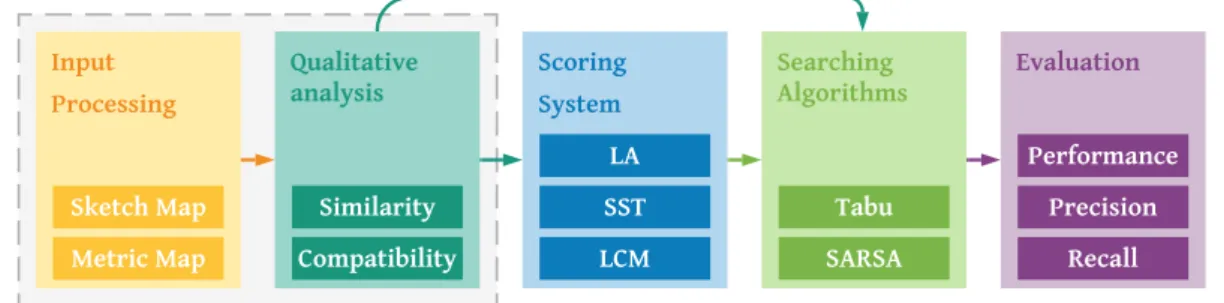
3.18 For each major component, every module is responsible for a set of process and outputs that are going to be used in future functionalities; this workflow is shown in Figure 7 with gray dotted lines for the modules used from the SmartSkeMa framework:

Figure 7 Thesis implementation workflow

3.2 SYSTEM SETUP

For workflow implementation, it is necessary to integrate different libraries and modules in a unique environment. For the system setup, the following libraries were used from and in the SmartSkeMa framework.

3.2.1 Python

The proposed methodology is developed in Python. Python is an object-oriented programming language with high-level data structures as it offers diverse standard libraries from string processing to system interfaces, some of which are specially design and optimized to handle large datasets (The Python Software Foundation, 2009).

The main Python libraries implemented are:

• Numpy (v. 1.18.1): package dedicated to scientific computing with Python offering tools for manipulating N-dimensional array datasets. We use the matrix tools to store, manipulate and process data (NumPyCommunity, 2020)

• Intertools (v. 2.3): this module offers fast and memory-efficient tools to iterate through data. As in our research, it is needed to search in large datasets. This module helps to optimize the process in between during the solution exploration (The Python Software Foundation, 2003b).

3.19 • Collections (v. 2.4): module implementing specially designed container datatypes as alternatives to the Python’s standard built-in ones, with a high-performance outcome in our case for storing and manipulating the data in the implementation (The Python Software Foundation, 2003a) • OpenAI Gym: a library with a collection of test problems called environments

to implement reinforcement-learning algorithms with a shared interface (Brockman et al., 2016)

3.2.2 SmartSkeMa framework

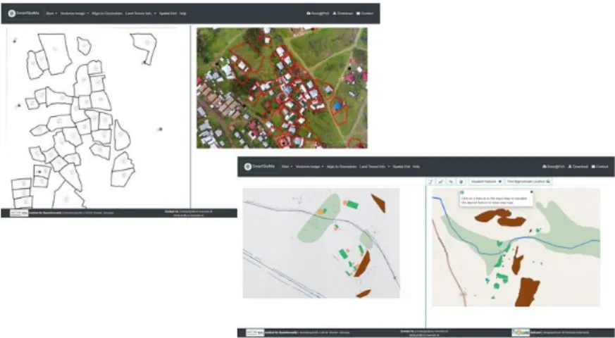
The Smart Sketch Map system (SmartSkeMa) is an application to record sketch-based information regarding land tenure in the frame of peri-urban and rural territories displaying an integrated vision of the end user’s sketch map and a cartographic dataset (M Chipofya, Jan, Schultz, & Schwering, 2017). An overview of the interface is displayed in Figure 8 with the input sketch map in the left and in the right side, the corresponding metric map.

Figure 8 SmartSkeMa interface

From the SmartSkeMa project, the main modules used are:

• Sketch recognition: for identifying distinctive elements in the sketch maps, for instance, water bodies, houses or mountains, the module processes shapes, and features’ representations by using a symbol recognizer to extract visual representations and transforming them into vector geometries (see Figure 9) to be stored in the system, using supervised learning techniques, polygonal clustering methods (Ng & Han, 2002) and

3.20 image recognition methods (K. Broelemann, 2011; Klaus Broelemann & Jiang, 2013)

z

Figure 9 SmartSkeMa vectorization

Through the interface, we provide the sketch and the metric map files and run the Automatic Vectorization process, and additionally, we provide more vectorized features using the Geometry Editor functionality. The interface described is displayed in Figure 10:

Figure 10 SmartSkeMa Geometry Editor user interface

• Qualitative Representation: In the sketch to map alignment problem, every item is defined as a node inside the qualitative map with a designated class and the corresponding attribute values to identify them. Spatial relations are used to describe the location of each item in the qualitative spatial representation, becoming labels between each node in a graph matching model, and only a set of qualitative calculus are combined with stabilizing the distortions captured from the sketch map (M Chipofya et al., 2017).

As a result, the module generates the corresponding Qualified Map for the sketch and the metric maps and the Similarity Matrices. Both datasets are organized based on the candidate pairs; these are each possible

3.21 combination between an element in the sketch map that may correspond to another element in the metric map. The Qualified Map dataset describes the labels between each node in the graph representation of the sketch to map association per relation set. On the other hand, the Similarity Matrix contains binary information about the compatibility between each label for every candidate pair.

3.2.3 Metric map generation

For the generation of the metric map’s dataset, the software QGIS in the version 3.10 A Coruña is used to digitalize the areas’ features and export them as a geoJSON file. QGIS is an open-source and multiplatform Geographic Information System (GIS) application supporting raster, vector, and database operations and functionalities for managing geographical information (QGISORG, 2002).

3.2.4 Execution environment

All the procedures were executed on an Intel Core i7-75002U CPU at 2.70GHz, and 8GB DDR4 memory card with a 19GB dedicated virtual memory. A set of environments with different Python configurations are created through Anaconda, a scalable data science multi-platform environment manager for packages and Python distributions, with an extensive collection of open source modules to find, access and share (Anaconda, 2020). An Anaconda environment executes a Python version 3.6.4 configuration along with the packages required to run the SmartSkeMa framework. This version of Python is selected according to TensorFlow’s version requirements for the Qualitative Segmentation Module.

3.3 INPUT DATASETS

Sketch mapping is a drawing exercise on a large piece of paper that allows recreating a global image of the people’s spatial distribution of their territory (Štěpánková, 1992) The following sketch maps are spatial representations with different complexity levels to test the proposed algorithms. All of them have been generated by humans on different platforms, with two of them with the same objective: describe an area of interest

3.22 according to the mental image of a space previously experienced. In the following subsections, a detailed description of each one is provided.

The common relevant attributes in these representations include: • smart_skema_type: type of feature according to the domain model

implemented in the SmartSkeMa framework, derived from the workshops carried in the Maasai community in Kenya for the its4land project (Karamesouti et al., 2018; Murcia, 2018). The features’ type catalog is detailed in Table 2.

• name: a descriptive label for each feature for identifying purposes • id: feature unique identifier for different processes inside SmartSkeMa

and the DPSM implementation.

Table 2 SmartSkeMa feature types

Feature type Description

beacon An object for specifying land boundary

boma A small place where people rest

boundary Clear delimitation of an area

house Standard family living unit

marsh Large wetland with plants. Associated to green _{areas in the experiment}

mountain Represents a single mountain or chain of _mountains

olopololi Area for agricultural activities. Associated to _{bridges in the experiment}

oltinka Water collection site

river Natural or human-made water currents

road Human-made access with or without pavement _surface

school Building with educational purposes

tree An area containing one or more trees

3.23

3.3.1 Artificial dataset

The artificial dataset is a set of different elements with a random distribution. In Figure 11, the resulting sketch map is displayed. On the left side is the sketch map representation, and on the right side, the objective metric map to align.

Figure 11 Artificial dataset SVG

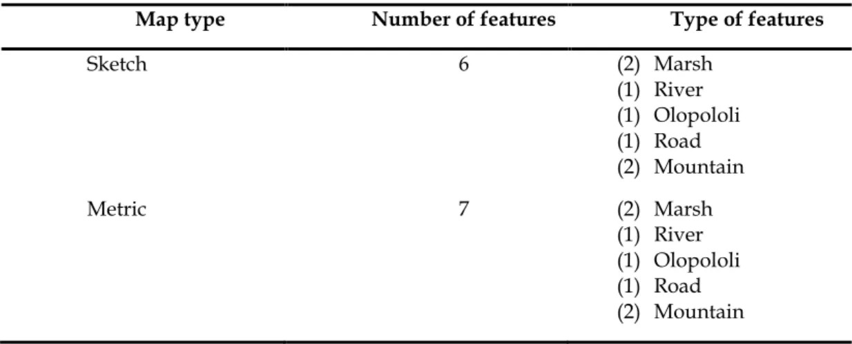
Each one of the map representations contains the features described in Table 3:

Table 3 Artificial dataset features

Map type Number of features Type of features

Sketch 6 (2) Marsh (1) River (1) Olopololi (1) Road (2) Mountain Metric 7 (2) Marsh (1) River (1) Olopololi (1) Road (2) Mountain

3.3.2 El Remanso

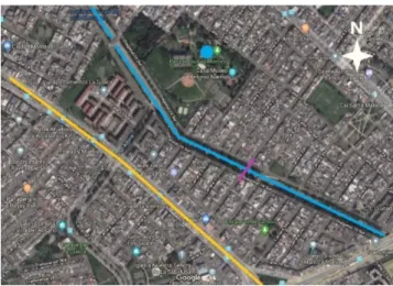
El Remanso is a small neighborhood located in Bogotá, Colombia, in a residential area between the Fucha river (blue line) and the Primera de Mayo Avenue (yellow line), as displayed in Figure 12. The community enjoys green areas around the river, such as the Ciudad Montes Park, which has a small lake (blue circle). People from the southwest side of the river can cross using a

3.24 bridge (purple line). Bogotá is known for the mountain chain in the east called Eastern Hills, as they are visible from most of the citizens and serves as an essential spatial reference element in the landscape (Pavony, 2000; Robson, van Kerkhoff, & Cork, 2019)

Figure 12 El Remanso neighborhood (Google Maps view)

The sketch map represents the mental image of the main elements recalled from the neighborhood, as shown in Figure 13:

Figure 13 El Remanso: sketch (left) and metric (right) maps

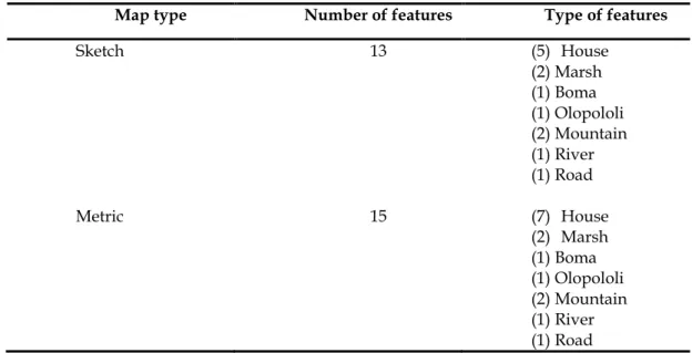
The metric map geoJSON file is created in QGIS A Coruña, and the attributes are filled according to the SmartSkeMa guidelines. Each one of the map representations contains the features described in Table 4:

3.25

Table 4 El Remanso dataset features

Map type Number of features Type of features

Sketch 13 (5) House (2) Marsh (1) Boma (1) Olopololi (2) Mountain (1) River (1) Road Metric 15 (7) House (2) Marsh (1) Boma (1) Olopololi (2) Mountain (1) River (1) Road

3.3.3 Mailua Ranch

The Mailua Ranch is a sketch map data set collected in the Maasai community located in Southern Kenya, in which the SmartSkeMa project participates with other partner universities to provide tools in the land rights for the area residents. The sketch map in Figure 14 was created by individuals from the Maasai community in one of the field studies where additionally the domain model was generated for the spatial components described including classes for environmental characteristics, social units, activities, shapes, housing, and farming (Karamesouti et al., 2018).

Figure 14 Mailua Ranch: sketch (left) and metric (right) maps

The sketch map object representations contain the features described in Table 5:

3.26

Table 5 Mailua Ranch dataset features

Map type Number of features Type of features

Sketch

(geometry editor) 16 (1) School (1) River (2) Road (3) Mountain (1) Marsh (3) Boma (5) Olopololi Sketch

(vectorization) 31 (1) School (1) River (2) Road (4) Mountain (5) Marsh (8) Boma (11) Olopololi Metric 106 (1) School (1) River (2) Road (3) Mountain (3) Marsh (n) Boma (n) Olopololi

3.4 QUALITATIVE ANALYSIS

The sketch to map features alignment is approached as a graph matching problem in which every map feature is defined as a node and each relation label as an edge, as described in section 3.2.2. In the SmartSkeMa Input Processing, the system generates the Similarity matrices and Qualitative Constraint Map (QCM) and stores them to be used in the Qualitative analysis module, responsible for providing the compatibility and the similarity evaluation between two candidate pairs during the execution of the searching algorithms.

A candidate pair p is a set of features (𝑖, 𝑖′_{) where i ∈ 𝑋 and 𝑖}′_{∈ 𝑌, in this}

case, with 𝑋 representing the sketch map and 𝑌 the metric map to align. The main tasks of this module are to return values for:

• Similarity: the similarity between the two pairs, 𝑝1 and 𝑝2 is recovered

3.27 𝑠𝑖𝑚𝑖𝑙𝑎𝑟𝑖𝑡𝑦(𝑝1, 𝑝2) = { 𝑇𝑟𝑢𝑒, 𝑖𝑓 𝑁 × 𝑁′ 𝑝1,𝑝2 = 1 𝐹𝑎𝑙𝑠𝑒, 𝑖𝑓 𝑁 × 𝑁′ 𝑝₁,𝑝₂ = 0 3. 1

• Type Compatibility: the type compatibility for a pair (𝑖, 𝑖′_{) is evaluated}

from the QCM feature type attributes QM as:

𝑡𝑦𝑝𝑒 𝑐𝑜𝑚𝑝𝑎𝑡𝑖𝑏𝑖𝑙𝑖𝑡𝑦(𝑖, 𝑖′) = {𝑇𝑟𝑢𝑒, 𝑖𝑓 𝑄𝑀(𝑖) = 𝑄𝑀(𝑖′)

𝐹𝑎𝑙𝑠𝑒, 𝑜𝑡ℎ𝑒𝑟𝑤𝑖𝑠𝑒 3. 2

• Candidate-Solution Compatibility: given a current solution 𝑚 , for a candidate pair 𝑝′ _{the compatibility with 𝑚 is:}

𝑐(𝑚, 𝑝′) = {𝑇𝑟𝑢𝑒, 𝑖𝑓 ∀ 𝑝 ∈ 𝑚 𝑠𝑖𝑚𝑖𝑙𝑎𝑟𝑖𝑡𝑦(𝑝, 𝑝′) = 1

𝐹𝑎𝑙𝑠𝑒, 𝑜𝑡ℎ𝑒𝑟𝑤𝑖𝑠𝑒 3. 3

The definition of these values helps to filter the search space during the selection of candidate pairs for a current solution to the ones who add value to the final solution.

3.5 SCORE SYSTEM

The evaluation of a pair is a critical process in the alignment problem as the decision of the next most fitting step must contemplate the impact of the extension of every QCN, each relation set, and additional considerations (Chipofya, 2013). In this thesis, the additional considerations are based on the graph matching solutions for discrete problems in a closed graph, which state the influence of the vicinity configuration (R. Battiti & Protasi, 2001). From the Similarity Matrix, a Link Analysis is used to extract the ranking scores of each node in terms of their connectivity, taking these results to extract an initial solution with the Spectral Solution Technique studying, in this case, the clustering behavior of the nodes. Finally, from the neighborhood properties of the LCM, two heuristic scores are calculated.

3.5.1 Page Rank

PageRank is an algorithm developed to ranking a node according to the number of links in a web graph, by assigning a score between 0 and 1; during the graph exploration, some nodes are more visited than others, creating a network in which profoundly explored nodes share a high number of connections in between. (Ceri et al., 2013; Page, Brin, Motwani, & Winograd,

3.28 1998a). The result is a distribution probability vector or also called the left-eigenvector, representing the ranking score for the candidate pairs in the Similarity Matrix A.

Consider a web graph G in which pages are represented by nodes 𝑁. Let 𝑢 be a web page (node) pointing to a set of pages (nodes) 𝐹𝑢 and in the

same way 𝐵𝑢 the set of nodes pointing to 𝑢. Let 𝐿𝑢 = |𝐹𝑢| be the number of

links (edges) from 𝑢 and 𝑐 to be a normalization factor. The equation gives the simplified version of PageRank ranking value R:

𝑅(𝑢) = 𝑐 ∑ 𝑅(𝑣) 𝐿𝑣 𝑣∈𝐵_𝑢

3. 4

In order to calculate the corresponding PageRank score, the following variables and procedures are addressed:

• Teleport operation: if 𝑁 is the total number of nodes in the web graph 𝐺, the operation to move from one to another happens with a probability of _𝑁1. A teleport rate with probability 0 < 𝛼 < 1 is defined to avoid looping in nodes with low compatibility and encourage exploration. • Initial probability distribution vector: base vector for the distribution

probability vector as it represents each node value procured by dividing the sum of the number of nodes connected to it by the total number of features connected. In the case of the sketch to map alignment, the number of nodes connected is the ones with value 1 in the Similarity Matrix, as it represents the compatibility of each one of the features in the search space.

• Transition Probability Matrix P: Consider a graph G with a set of nodes N= {A, B, C}. The matrix P represents the distributed probability of moving from one node to another, as seen in Figure 15:

3.29 A row represents a candidate pair in the Similarity Matrix, and it is divided by the number of compatible features in that row. For the resulting base matrix P, a Teleport Distribution ( 1 − 𝛼 ) and Teleport Variation (𝛼/𝑁) is applied.

• Power iteration: the method implemented to calculate the left-eigenvector and the corresponding largest eigenvalue of a matrix, named the Distribution Probability Vector, the ranking score. Some of the advantages of this method include that it does not affect the transition probability matrix P, can handle large sizes of data, and it returns the values of interest in less computational and complexity expenses.

The Link Analysis (PageRank) score computation in DPSM is executed with the Similarity Matrix, calculated from the input sketch and metric maps, as an argument, and the system retrieves the ranking scores for all candidate pairs. The link analysis results are used in the Spectral Score Technique (SST) as an argument to calculate an initial solution and, in the Tabu Search, to make a move in the selection process. In Figure 16, the PageRank implementation for the sketch to map aligning problem is detailed.

3.30

3.5.2 Spectral Solution Technique

The Spectral Solution Technique is an algorithm from Leordeanu and Hebert's research, able to find secure correspondences between a pair set of features as nodes in the graph matching problem, by calculating the eigenvector of a graph matrix M and processing these scores to get a collection of highly linked assignments. In this algorithm, selected features are highly related and expose high links scores showing a clustered behavior among them. On the other hand, low related features do not show any links rates, or if they appear, they show a considerable distance concerning the central cluster (Leordeanu & Hebert, 2005).

Consider a graph G with a set of nodes N represented by the matrix A. Initially the similarity matrix is constructed, followed by the definition of environment variables: L as the number of nodes, x as the elements of the row in the iteration, and x* the maximum eigenvalue or affinity scores for the Similarity Matrix M. As the SST addresses the use of maximum eigenvalue, it makes use of an algorithm that pursues the identification of links between large amounts of objects connected. One approach is Google’s algorithm, PageRank, which calculates a feature relevance inside a network according to the number of links shared with other features (Page, Brin, Motwani, & Winograd, 1998b). The algorithm will reject all the objects in the iteration with a lower value and a corresponding label in conflict with x* and collect the high scored and compatibles ones as long there are features left to analyze in L. Finally, x will contain the pairs candidates with the highest confidence of being correct assignment. The algorithm executes the steps described in Figure 17. In general, in the graph matching problem, the SST candidate pairs serve as a start point for the exploration in the search space. For the sketch to map alignment, these selected features represent the pairs candidates with the most number connections or relation labels inside the sketch-metric map graphs being good candidates for initializing the search. Moreover, according to the Link Analysis theory and Leordeanu findings, from the analysis of the candidate pair’s vicinity and identifying the existence of robust correlated features, the definition of the first steps during the search task make the results more profitable than resume from a point with no information available (R. Battiti & Protasi, 2001).

3.31

Figure 17 Diagram for the Spectral Solution Technique algorithm

3.5.3 Heuristic scores from LCM

The third score component is based on the properties of the Local Compatibility Matrices described in section 2.3.3, especially the non-overlapping labels property in which matrix cell with the same label generate a non-overlapping square submatrix inside the LCM from which two heuristic scores are derived (Malumbo Chipofya et al., 2013):

Consider a candidate pair (𝑖, 𝑖′_{) with LCM ℒ}

(𝑖,𝑖′₎and its corresponding

submatrices denoted by ℒ_(𝑖,𝑖′_),𝑅 with rows 𝑟𝑜𝑤𝑠(ℒ_(𝑖,𝑖′_),𝑅) and columns

𝑐𝑜𝑙𝑠(ℒ_(𝑖,𝑖′_),𝑅), where R is a label 𝑅∁𝑹. The first observation of this configuration

is the possibility of identifying a set of submatrices inside ℒ_(𝑖,𝑖′₎ furthermore

3.32 dimension which indicates the highest contribution of each ℒ_(𝑖,𝑖′_),𝑅 into the

extension of the current candidate pairs match 𝑚 in the future: the highest the total sum of the min dimension of the submatrices in the LCM, higher the chances to find in the future more compatible candidates in the solution as indicated in the equation:

𝑒𝑣𝑎𝑙𝑖,𝑗|𝑚= ∑ min (dim (ℒ(𝑖,𝑖′)(𝑅)))

𝑅∁𝑹 3. 5

The result is a greedy selection of candidate pairs, as the selection follows the paths labeled as useful in the first consideration. The second heuristic H2 complements the first heuristic H1 by providing a peak in the estimation of a good pair in the solution evaluating the impact of the current pair (𝑖, 𝑖′_{) into future solutions by ordering the candidate pairs in ascending}

order of H1 and considering the most significant feature, ℎ𝑒𝑎𝑑𝑖 as the possible

solution that contains the node (𝑖) (M. C. Chipofya et al., 2016) as described in the equation:

𝑐𝑜𝑢𝑛𝑡𝑘(𝑚) = |{𝑖 ∈ 𝑁|𝑘 ≤ 𝑒ℎ𝑒𝑎𝑑𝑖|𝑚}| 3. 6

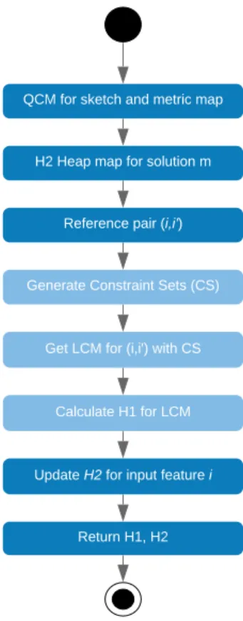
In the DPSM implementation, the first heuristic is calculated by recovering the LCM from the Qualitative Constraint Map (QCM) for a set of candidate pairs. The result is a batch of scores indicating the value of H1 per each relation set identified from the QCM and finally summarizing them to get a global score. Secondly, the heuristic H2 is updated for the input map (sketch map) and extended by the SmartSkeMa framework, merging the implementation of the first heuristic. The procedure happens as the candidate pairs are evaluated during the calculus of H1, maintaining an updated score structure as the search is executed, adding new features into the solution. Figure 18 describes the implementation for generating the LCM and calculating the H1 and H2 scores:

3.33

Figure 18 Heuristic scores calculation workflow

3.6 SEARCHING ALGORITHMS

The aligning of a sketch map feature to a feature in a metric map is the examination of a large set of options that comply with specific characteristics to be a good match. We explore all the options on the metric map to find which one is the most like to match a specific feature in the sketch map. Diverse techniques from non-learning and learning algorithms have arisen from research. In this thesis, we implement two different search algorithms, with different approaches, advantages, and configurations: a Tabu Search and a SARSA, an incremental dynamic programming algorithm to solve reinforcement learning problems (Saad, 2011).

3.6.1 Tabu Search

Tabu search approach is to solve combinatorial optimization problems like the ones in graph theory by using a list of banned or taboo moves obtained from a number of iterations in a local search to construct a final solution (Roberto Battiti & Tecchiolli, 1994; Glover, 1989a).

3.34 For the configuration of the Tabu algorithm, the main arguments are the search space, the local search space or neighborhood, the list of banned moves, and the criteria to establish whether they belong to the current solution or need to be penalized at each iteration. An overview of the general workflow is shown in Figure 19:

Figure 19 Tabu Search workflow diagram

In the context of the sketch to metric map alignment, the overview for each of these aspects and their processing is as follows:

• Search Space: the space of every possible item that can be contemplated as part of the final solution during the search (Gendreau & Potvin, 2005). For the interest of this study, the search space is all possible combinations 𝑚 composed only by compatible candidate pairs 𝑃 = (𝑖, 𝑖′) where 𝑖 and 𝑖′ represent a feature from the sketch and metric map.

3.35 • Current solution: denoted by 𝑆. The solution used as the initial one is the

output from the Spectral Solution Technique.

• Neighborhood: the set of available pairs to add to the current solution. For each iteration, a modification or move is applied to the solution 𝑆 to add or remove a pair. The result is a collection of available compatible pairs called neighboring solutions, a subset of the search space. The evaluation of items belonging to the neighboring solutions is done using the functions created in the Qualitative Analysis module. Each new pair added to the current solution 𝑆 during the Tabu Search is compared to every item in the search space 𝑆 to check their compatibility. If old items are not compatible with the most recently added one, they are removed. In the same way, if items from the search space are compatible with the recently added one and with the remaining items, the neighborhood is updated with new available moves.

• Move: for each iteration, the algorithm performs a modification to the currently available solution considering all potential actions. For the current implementation, two actions are possible: ADD or REMOVE. The criteria for choosing one or another depends on the evaluation of the neighborhood explained in the following points. The dynamics of a move during the search are displayed in Algorithm 1.

Algorithm 1. Tabu Search

input: 𝑆0, number iterations iter, LA, QSM, QMM, metric_size

output: 𝑆

// initialize

1 Set S=initial solution S0;

2 Set tabu_in list; 3 Set tabu_out list; 4 while iterations

5 Update available moves

6 Select best non-tabu available move 7 if move is ADD

8 Insert move into S

9 Insert move into tabu_out 10 else move is REMOVE

11 Remove move from S

12 Insert move into tabu_in 13 return best matching result S

3.36 • Best non-tabu available move (best_move): for each iteration, the item with the highest LA score in the neighborhood is selected as the best candidate to be considered in the current solution 𝑆.

• ADD pair: the search next action is said to be ADD if the best_move does not exist in the current solution. The new pair is evaluated using the Qualitative Analysis module. For each item in the neighborhood, it assesses the Candidate-Solution and Types Compatibility values. If both values are positive, the pair is added and labeled as best_add.

• REMOVE pair: the search next action is said to be REMOVE if best_move already exists in 𝑆 or there are not useful items to be added in the current solution 𝑆, with not useful meaning a candidate pair that is incompatible with one or more features in 𝑆 . The procedure is to discard the item with the lowest LA score in 𝑆, named best_remove.

After executing an ADD or REMOVE move, in both cases, the output element, best_add or best_remove, is appended to a tabu list. In this implementation, two lists are created: tabu_in and tabu_out.

• Tabu lists update: These are managed by a FIFO (First-In, First-Out) method; each time a new element is added to the bottom of the list, the first added element on the list is removed (Glover, 1986). The tabu_in list manages the items that we discarded from 𝑆 and tabu_out list the ones we join to the solution. At the beginning of each iteration, the available moves are updated additionally by removing the items in the tabu lists. Instead of using a unique list, we implemented two list, this with the objective of encouraging exploration but on the other hand to not over consider useful elements into the solution, this approach seems to have an advantage in terms of the activity of each list in the algorithm assuring no duplicated solutions while considering candidates inside the solution 𝑆 (Glover, 1986, 1989b). The size of the tabu lists is fixed to 25% of the size of the current solution.

The algorithm search is executed, and for a given number of iterations, it explores a set of solutions, adjusts the initial solution 𝑆 by adding or removing pairs from a neighborhood 𝑁(𝑠) of 𝑠, appearing according to the compatibility to a new solution 𝑆′. (Glover, Taillard, & Taillard, 1993). Finally,