Similar understorey structure in spite of edaphic and
floristic dissimilarity in Amazonian forests
Lassi SUOMINEN1*, Kalle RUOKOLAINEN1, Timo PITKÄNEN2, Hanna TUOMISTO1
1 University of Turku, Department of Biology, FI-20014 - Finland
2 University of Turku, Department of Geography and Geology, FI-20014 - Finland * Corresponding author: lasasu@utu.fi
ABSTRACT
Forest structure determines light availability for understorey plants. The structure of lowland Amazonian forests is known to vary over long edaphic gradients, but whether more subtle edaphic variation also affects forest structure has not beenresolved. In western Amazonia, the majority of non-flooded forests grow on soils derived either from relatively fertile sediments of the Pebas Formation or from poorer sediments of the Nauta Formation. The objective of this study was to compare structure and light availability in the understorey of forests growing on these two geological formations. We measured canopy openness and tree stem densities in three size classes in northeastern Peru in a total of 275 study points in old-growth terra firme forests representing the two geological formations. We also documented variation in floristic composition (ferns, lycophytes and the palm Iriartea deltoidea) and used Landsat TM satellite image information to model the forest structural and floristic features over a larger area. The floristic compositions of forests on the two formations were clearly different, and this could also be modelled with the satellite imagery. In contrast, the field observations of forest structure gave only a weak indication that forests on the Nauta Formation might be denser than those on the Pebas Formation. The modelling of forest structural features with satellite imagery did not support this result. Our results indicate that the structure of forest understorey varies much less than floristic composition does over the studied edaphic difference.
KEYWORDS: canopy openness; Iriartea deltoidea; Pebas Formation; pteridophytes; stem density
Similaridade na estrutura do subosque a despeito de dissimilaridades
edáficas e florísticas em florestas da Amazônia
RESUMO
A estrutura florestal determina a disponibilidade de luz para plantas do subosque. Nas planícies Amazônicas, a estrutura florestal varia com fortes gradientes edáficos. O possível efeito de variações edáficas mais sutis sob a estrutura das florestas não está resolvido. Na Amazônia ocidental, a maioria das florestas não-inundadas crescem em solos derivados de sedimentos relativamente férteis da Formação Pebas ou de sedimentos mais pobres da Formação Nauta. Nosso objetivo é comparar a disponilidade de luz e a estrutura do subosque de florestas crescendo sobre duas formações geológicas. Nós medimos a abertura do dossel e a densidade de troncos de árvores em três classes de diâmetro no nordeste Peruano, totalizando 275 pontos de estudo em florestas de terra-firme representando as duas formações geológicas. Além disso, documentamos as variações na composição florística (samambaias, licófitas e a palmeira Iriartea deltoidea) e utilizamos informações de imagens de satélite Landsat TM para modelar as características estruturais e florísticas das florestas em uma área mais ampla. A composição florística sobre as duas formações foram claramente distintas e isso também pôde ser modelado com as imagens de satélite. Já as observações de campo sobre a estrutura da floresta deram uma fraca indicação de que as florestas sobre a Formação Nauta poderiam ser mais densas do que as florestas sobre a Formação Pebas. A modelagem das caraterísticas da estrutura florestal com imagens de satélite não deram o mesmo resultado. Nossos resultados indicam que a estrutura do subosque varia muito menos do que composição florística no gradiente edáfico estudado.
INTRODUCTION
Forest structure is an important habitat feature for a variety of organisms. The structure of forest understorey influences light availability at the ground layer, and is therefore an important variable for undestorey plants and young individuals of canopy trees (Nicotra et al. 1999). Some Amazonian forests growing on soils with strongly different nutrient concentrations and/or drainage conditions are known to differ markedly in structure (Pires and Prance 1985; de Carvalho et al. 2013), but there is little evidence for more subtle soil-related structural variation (Baraloto et al. 2011).
A large part of non-inundated terra firme forests in western Amazonia grow on soils formed in one of two geological formations, the Pebas Formation and the Nauta Formation. The clayey Pebas Formation sediments have relatively high concentration of base cations (Ca, K, Mg, Na), whereas the loamy to sandy Nauta formation sediments have about one order of magnitude lower cation concentration (Hoorn 1993; Rebata et al. 2006; Hoorn et al. 2010). Higgins et al. (2011) found that at least half of the most common tree, Melastomataceae and pteridophyte species have statistically different abundances or frequencies between forests on the two geological formations. The vegetation map of Brazilian Amazonia (Veloso et al. 1974; IBGE 2004) divides terra firme forests into two main types, which have structural terms floresta aberta and floresta densa (open forest and dense forest, respectively). At least in western Brazilian Amazonia, the border line between these forest types coincides with the limit between the Pebas and Nauta Formations (in Brazilian terminology: Solimões and Içá Formation, respectively; Higgins et al. 2011). However, there is no quantitative or qualitative documentation of possible structural differences between floresta densa and floresta aberta.
High cation concentration is a general indication of relatively high fertility of soil. Therefore it can be expected that average tree growth rates are higher, life-spans shorter and thereby the rate of appearance of new gaps is faster in forests on the relatively cation-rich Pebas Formation than on the cation-poorer Nauta Formation (Malhi et al. 2006; Quesada et al. 2012). On the other hand, faster growth rates might close the gaps faster on the Pebas Formation, so it is not obvious whether one should expect a difference in forest understorey structure or not.
The objective of this study was to compare structure and light availability in the understory of forests growing on the Nauta and Pebas Formations. To address this question, we used both field measurements of forest structural variables and spatial modelling based on satellite images.
MATERIALS AND METHODS
Study area and sampling
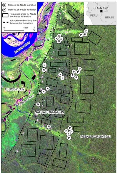
Our study area is located ca. 50–75 km SE of Iquitos in northern Peruvian Amazonia (Figure 1). There is a previously mapped boundary between the Nauta and Pebas Formations (Kalliola et al. 1998; INGEMMET 1999), and old-growth forests are relatively easily accessible on both formations.
Field sampling was made in old-growth forests along 500-m-long inventory transects. The minimum distance between transects was 500 m. We established 25 transects, 12 on the Nauta Formation and 13 on the Pebas Formation. Transect locations were selected on the basis of accessibility and a preliminary interpretation of the satellite image. The transects were established by opening in the forest understorey an approximately 1-m-broad baseline trail following a pre-defined compass bearing. Transect length was measured with a 50-m measuring tape. The first observation point was established at the starting point, and thereafter observation points were at 50-m intervals for a total of 11 points per transect. The observation points were located 10 m off the transect base line alternating between the left and right side. Three observation points per transect, one in each end and one in the middle, were georeferenced with a hand-held GPS. Coordinates of the remaining points were calculated based on the GPS-referenced locations, spacing them at even intervals between the end and the middle points.
Forest structural data
At each observation point, we measured four variables: canopy openness and the densities of self-supporting woody plants (including palms) in three size classes. The size classes were defined by diameter at breast height (DBH) and were saplings (DBH ≤ 2.5 cm), poles (2.5 < DBH < 10 cm) and trees (DBH ≥ 10 cm). Most previous forest structural studies include only trees ≥ 10 cm DBH. We chose these size classes since we think that the density of saplings and poles is an important habitat characteristic for understorey organisms.
per hectare for each observation point was obtained as the sum of the densities in all three size classes.
In total, we measured the forest structural variables in 275 observation points (132 on Nauta Formation and 143 on Pebas Formation). For each forest structural variable, we calculated its transect-wise arithmetic average based on the 11 points per transect.
Floristic data
We wanted to cross-check that our field study sites really represent the two distinct geological formations. Therefore, we inventoried pteridophytes (ferns and lycophytes), that are
good indicators of soil properties in Amazonia (Tuomisto et al. 2003; Higgins et al. 2011). Additionally, we surveyed the distribution of the palm Iriartea deltoidea Ruiz and Pavon, which has been reported to be an ecological generalist and abundant over wide areas of western Amazonia (Pitman et al. 1999; Pitman et al. 2001; Kristiansen et al. 2012).
Within a radius of approximately 10 m from each observation point, the three most abundant terrestrial or low-epiphytic (lowermost leaf less than 2 m above the ground) pteridophyte species were registered and photographed by LS. If two pteridophyte species appeared to have equal numbers of individuals inside the circle, the species with an individual
closer to the central point was deemed to be more abundant. Species identification was done after the fieldwork by HT on the basis of the photographs. All but 13 specimens could be identified to species (or morphospecies) and only one juvenile could not be identified even to genus. The occurrence of the palm Iriartea deltoidea was surveyed within a 5-m-wide corridor along each 500-m-long inventory line by counting the number ofindividuals that had a trunk of at least 1 m tall.
Satellite image data
Field sampling can only produce point data, but we aim to make generalisations about the Nauta and Pebas Formations. We wanted to assess how representative our field inventory transects were of the Nauta and Pebas Formation more broadly. Therefore we investigated how the characteristics of our field study sites as seen in a Landsat TM satellite image relate to the surrounding areas where these two geological formations had been mapped by Kalliola et al. (1998) and INGEMMET (1999). We addressed this question by two means. Firstly, we used the satellite image data to develop a simple predictive model for plant species composition and for each forest structural feature and in the study area, and secondly, we investigated if the spectral data of our field inventory transects can be considered a representative sample of spectral signatures of corresponding transects in the study area in general. Landsat imagery was chosen because it is free-of-charge and has been shown to correlate with edaphic, floristic and forest structural patterns in Amazonian forests (Lu et al. 2004; Higgins et al. 2012).
We used the cloud-free Landsat TM image (path 006, row 063, 20 June 2011) that was temporally closest to the collection of field data (January-April 2010) to obtain spectral information in the bands 1–5 and 7. We registered digital numbers from pixels that touched a 50 m buffer around the observation points. For each transect and Landsat band, we calculated the average value of its pixels for all the six bands. One Nauta Formation transect was partly covered by clouds and was therefore left out of this analysis.
We defined cloud-free rectangular reference areas for each formation in relatively homogeneous-looking old-growth forest areas (Figure 1). Within the reference areas, we delineated 2098 reference transect windows that were of similar size and shape as the windows drawn around the field inventory transects. The average spectral signature was registered for each reference transect window.
Numerical analyses
We tested for spatial autocorrelation in forest structural variables by calculating Moran’s I. The lag distance was set to the longest distance between any two adjacent observation points (59.41 m, measured from the calculated positions of the observation points on the satellite image). We tested the statistical significance of Moran’s I using 999 permutations under the total randomization model.
To measure the difference in the distribution of canopy-scope scores between Pebas and Nauta Formation we divided the canopy-scope scores into three bins: small gaps (score 1-2), medium gaps (3-8) and big gaps (9-16) (Figure 2). We then calculated the percentage of canopy scope scores in each
bin for each geological formation separately. The statistical significance of the difference was tested by permutation.
We calculated pairwise Spearman rank correlations between all forest structural variables and tested the statistical significance of the difference in log-transformed mean stem density per observation point between the Pebas and Nauta Formations with Welch two-sample t-test. We investigated the power of the t-tests with a power analysis function for unequal sample sizes and estimated how large a difference in log-transformed mean stem density between the geological formations would be detectable with an 80 percent probability given the present standard deviation, sample size and significance level. The tests were performed with log-transformed variables, but we report the results back-transformed, i.e. as the ratio between the geometric means of the original variables.
We compared the variances of forest structural variables between Nauta Formation and Pebas Formation with Levene’s test. We standardised the variables and calculated the variance for each variable on each formation separately and calculated the sum of these variances for each formation. We estimated the probability of getting by chance a difference in variance sum equal to or larger than the observed one by permuting the standardised variables 999 times.
We used the transect-wise presences and absences of pteridophyte species to compute pairwise Sørensen index values (Sørensen 1948) and used their one-complements to illustrate the compositional dissimilarities among transects with a two-dimensional nonmetric multidimensional scaling (NMDS; Legendre and Legendre 1998). The t-test, Levene’s test, power test and the NMDS ordination were made with R 2.15.0, using the packages stats, car, pwr and vegan, respectively (Champely 2009; Fox and Weisberg 2011; Oksanen et al. 2012; R Development Core Team 2012).
We used multiple regression analysis to model forest structural variables and pteridophyte species composition (represented by the coordinate score of field transects in a one-dimensional NMDS) as a linear function of the spectral signatures in the six bands. Stepwise multiple regression was used in order to select only statistically significant explanatory variables. Both backward and forward selection were used, and the bands were ranked according to Akaike’s information criterion. The function stepAIC in the MASS package of R (Venables and Ripley 2002) was used. We applied these models to predict the forest structural variables over the reference transect windows. Extrapolation was avoided by removing all reference transect windows that had spectral signatures outside the range observed in the field inventory transects.
Finally, we estimated if our field sampling gives a possibly biased view of the difference between the two geological formations. To this end we investigated if the spectral difference between the geological formations was similar when measured on the basis of the spectral signature of our 25 field study
transects or the 2098 reference transects. Using the six bands of the Landsat TM images, we constructed six-dimensional spectral spaces corresponding to the reference transects in the Nauta Formation, reference transects in the Pebas Formation, field transects in the Nauta formation and field transects in the Pebas Formation. By comparing the Euclidean distances between the corresponding spectral space centroids, we were able to evaluate if the field transects under- or overestimate the regional difference between the two geological formations.
RESULTS
Forest structure
We found that neighbouring observation points were no more similar in forest structural variables than observation points further away (Moran’s I ranged from -0.059 to -0.005 and the associated P-values ranged from 0.38 to 0.98). This indicates that the variables were not spatially autocorrelated, so we treated the observation points as independent observations in the subsequent analyses.
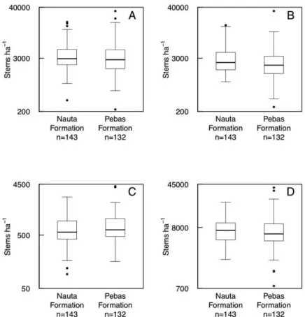
The forest structural features were generally not strongly correlated with each other (Table 1). Canopy openness was negatively correlated with the density of trees. The densities of saplings and poles were positively correlated. The geological formations did not differ significantly from each other in the frequencies of small, medium or big canopy gaps (Figure 2; Table 2). Only two forest structural features in our field data showed a statistically significant difference between the two geological formations. Mean density of poles was higher in forests on the Nauta Formation (t = 2.7, P<0.01) and variance in the density of trees was higher in forests on the Pebas Formation (Figure 3; Table 3). The sum of standardised variances of all four forest structural variables was higher in Pebas forests (4.67 vs. 3.26), but this difference was not statistically significant (999 permutations, P=0.196).
Table 1. Spearman rank correlation coefficients between forest structural variables using 275 observation points.
Poles Trees ≥ 10 cm DBH
Total stem density
Canopy openness
Saplings 0.18* 0.05 0.75*** -0.06
Poles -0.05 0.66*** -0.01
Trees ≥ 10 cm DBH 0.10 -0.23**
Total stem density -0.08
Bonferroni –corrected P-values: *P<0.05;**P<0.01;***P<0.0001
Table 3. Means and standard deviations (SD) of forest structural variables on the Nauta and Pebas Formations. The P-values are based on the two-sample t-test between the formations. The F-statistics and associated error probabilities are based on Levene’s test for homogeneity of variances between the formations.
Variable Nauta Formation Pebas Formation Levene’s test All observation points
Mean SD Mean SD F273 Pr(>F) Mean SD
Saplings 3965 3139 4028 4137 1.79 0.18 3998 3685
Poles 3363** 2714 2863** 3214 0.47 0.49 3103 2989
Trees ≥ 10 cm DBH 704 425 812 581 3.91 0.049* 760 514
Total stem density 8033 3956 7703 5350 1.78 0.18 7861 4727
Canopy openness 2.52 2.39 2.27 2.33 0.65 0.42 2.39 2.37
*P<0.05;**P<0.01
Table 2. Percentage of canopy-scope scores per formation falling into each of the three bins, and the permuted probability values for the percentual difference between the formations. For Nauta Formation N=132, for Pebas Formation N=143.
Bin Nauta Formation Pebas Formation P (999 permutations) Small gaps
(score 1 –2) 70.5 79.0 0.14
Medium gaps
(score 3–8) 25.8 16.8 0.08
Big gaps
(score 9–16) 3.8 4.2 0.97
Floristic composition
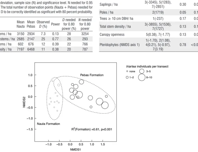
In total, 77 pteridophyte species were recorded in the transects. Of these, 43 species were recorded only on the Pebas Formation and 22 species only on the Nauta Formation. Twelve species were recorded on both formations. The mean species number per transect was 14.2 on the Pebas Formation and 10.5 on the Nauta Formation. In contrast to the inconclusive results on forest structure, floristic analyses gave very clear results. Pteridophyte species composition placed the transects into two clearly distinct groups in the NMDS ordination, and these groups corresponded perfectly with the limit that was drawn a priori between the two geological formations. In addition, we found only one individual of
Table 4. Statistical power of the stem density t-tests for significance level 0.05 (N=132 for Nauta Formation, N=143 for Pebas Formation). The t-tests themselves addressed arithmetic means of log10-transformed variables. For easier interpretation, the table shows the back-transformed values, i.e. the means are geometric and differences (D) are expressed as the percentage by which the larger mean exceeds the smaller mean. Power = 1-P(Type II error), i.e. the probability of correctly rejecting a false null hypothesis with the observed standard deviation, sample size (N) and significance level. N needed for 0.95 power = The total number of observation points (Nauta + Pebas) needed for observed D to be correctly identified as significant with 80 percent probability.
Variable Mean Nauta
Mean Pebas
Observed D (%) Power
D needed for 0.80 power (%)
N needed for 0.80
power Small stems / ha 3150 2934 7.3 0.13 28 3254 Medium stems / ha 2685 2147 25 0.77 26 293 Large stems / ha 602 676 12 0.39 22 766 Total density / ha 7197 6468 11 0.38 20 787
Table 5. The best linear regression models between forest structural variables, pteridophyte species composition and Landsat spectral signatures. Only models that had a statistical error probability of less than 0.05 were used to model forest structural variables for the reference transects.
Variable Selected bands (regression coefficient)
Adjusted R2
P (model)
Saplings / ha 3(-3345), 5(1283),
7(-2851) 0.30 0.02
Poles / ha 2(1719) 0.05 0.14
Trees ≥ 10 cm DBH/ ha 1(-237) 0.17 0.02
Total stem density / ha 3(-3855), 5(1536),
7(1727) 0.13 0.12 Canopy openness 5(0.38), 7(-1.77) 0.13 0.09
Pteridophytes (NMDS axis 1)
1(-1.70), 2(1.08), 4(0.21), 5(-0.97),
7(3.19)
0.78 <0.0001
the palm species Iriartea deltoidea in the Nauta Formation transects, which contrasts with the 58 individuals found in the Pebas Formation transects (Figure 4).
Satellite image analysis
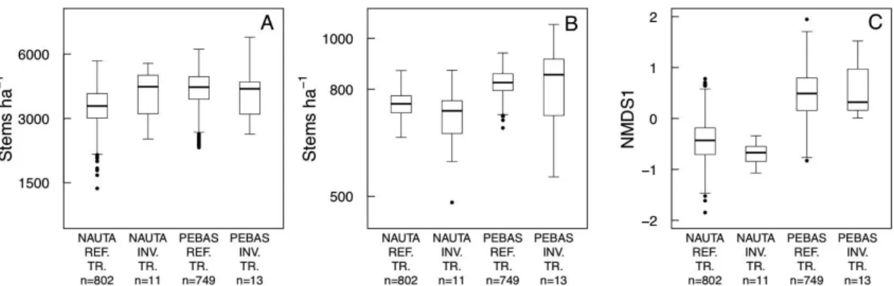
When satellite image data of the inventory transects were used to model forest structural charateristics and pteridophyte species composition, only the regression models for saplings, trees and pteridophytes were statistically significant (Table 5). Pteridophyte species composition was much better predicted by the spectral signatures than the forest structural variables were. By looking at the predictions of the statistically significant models (Figure 5), one can observe that the models for trees and pteridophyte species composition gave
predictions that coincided with the observed differences between the two geological formations. In contrast, the model for saplings predicted a difference that was opposite to the observed one. According to the model, sapling density on the Pebas Formation is clearly higher than on the Nauta Formation, whereas the field observations suggested that sapling density is slightly higher on the Nauta Formation.
The Euclidean distance between the centroids of the the six-dimensional spectral spaces corresponding to the two geological formations was shorter for the field transects than for the reference transects (distances 0.50 versus 1.21, respectively). This indicates that the field transects may have underestimated differences between the geological formations.
DISCUSSION
Similar understorey structure in spite of edaphic and floristic dissimilarity
We found very little evidence of differences in forest understorey structure between the Nauta and Pebas Formation. Especially the canopy scope measurements – our most direct measure of understorey light regime – were remarkably similar between the forests of the two geological surfaces. The lack of structural differences contrasts with floristic results that showed substantial and consistent compositional differences between the two formations both in our study and in previous ones (Ruokolainen and Tuomisto 1998; Higgins et al. 2011). The distinctness of the two floras is further supported by our observation that the palm Iriartea deltoidea was almost completely lacking from the Nauta Formation, although it was common on the Pebas Formation. This species has been described as a broadly distributed habitat generalist and the most dominant of the ‘oligarch’ species proposed to be ubiquitous in western Amazonian forests (Pitman et
al. 1999; 2001). A recent study reported Iriartea to occur without habitat preference in our study area (Kristiansen et al. 2012). Our contrasting results may arise from our focus on the occurrence of only relatively big individuals, or then from some local historical reasons that have temporarily reduced the abundance of the species in the forests of the Nauta Formation. Asner et al. (2013) reported from southern Peru that lowland rain forest canopy gap fequency and size distribution was practically invariable over different geological surfaces. This together with our results supports the idea that tropical rain forest structure changes much less readily in response to spatial variation in soil nutrient status than species composition does (Tuomisto et al. 2003; DeWalt and Chave 2004; Paoli et al. 2008). However, this study focused on stems thinner than 10 cm DBH. All stems thicker than 10 cm DBH were treated as one size class and therefore eventual differences in the density of some larger size classes may have gone unnoticed. It is also possible that eventual differences in forest structure between the two geological formations is not only related to different soil nutrient levels. The two formations differ also in their topography so that the Nauta Formation is characterized by a much flatter terrain than the Pebas Formation (Ruokolainen and Tuomisto 1998). Topography as such affects both mortality rate and the mode of dying of rain forest trees of different size classes (Toledo et al. 2011), and thereby forest structure may also vary only because trees die differently on different topographical positions.
The only statistically significant difference in forest structure that we found between the Nauta and Pebas Formation was that the average density of poles was higher on Nauta than on Pebas Formation. This result appears to conform with the current Brazilian forest classification (IBGE, 2004), which uses the term florestadensa (dense forest) for forests that occur mainly on the Içá formation and the term florestaaberta (open
forest) for forests on the Solimões formation. These formations correspond in terms of age and sedimentological environment to the Nauta Formation and the Pebas Formation, respectively (IBGE 2004; Schobbenhaus et al. 2004). Also, it has been found that stem density in Amazonian forests is weakly negatively correlated with soil Ca and Mg concentrations but positively correlated with soil K concentration (Quesada et al. 2012). However, several structural features that we studied did not give any indication that forests on the Nauta Formation would be denser than forests on the Pebas Formation. The modelled densities of both saplings and trees were actually higher on the Pebas Formation than on the Nauta Formation, but the explanatory power of the models was rather low: they explained 30 percent and 17 percent of the variation in the density of saplings and trees, respectively.
Based on our results, the formations do not seem to differ in canopy openness, although soil type may influence tree fall via soil texture, hydrology and fertility (Lobo and Dalling 2013). Forests on soil types that become unstable when water-saturated are more prone to gap formation. Also, more fertile soils favor tree traits such as fast growth and low wood density that promote gap formation (Quesada et al. 2012). In our case, this would be the case on Pebas Formation soils that are more fine-grained, less well drained and more fertile than the Nauta Formation soils. Quesada et al. (2012) suggested that, on a long nutrient gradient and excluding white-sand forests, nutrient-rich forests are on average more open than nutrient-poor forests.
Studies focusing on the relationships between forest structure and soil characteristics in tropical rain forests have yielded inconclusive or even contradictory results (Laurance et al. 1999; Slik et al. 2010; Baraloto et al. 2011). Gentry (1982) found stem density to be constant over seven different Neotropical forests. Vitousek and Sanford (1986) concluded that soil nutrients probably affect forest structure only in extreme cases. High stem density has been shown to be associated both with low (DeWalt and Chave 2004; Paoli et al. 2008) and high soil fertility (Slik et al. 2010). Baraloto et al. (2011) concluded that the density of small stems is often associated with low fertility whereas the density of large stems is associated with high fertility. Relative to these studies, our study compares forests of low and intermediate-high fertility (Ruokolainen and Tuomisto 1998; Higgins et al. 2011) and, perhaps not surprisingly, fails to find significant differences in average stem density. Neither did we observe any significant difference in the variance of stem density.
Stem density measurements and light availability
Our measurements of stem density seem somewhat inflated compared to other measurements of stem density in similar size classes in Amazonia (DeWalt and Chave 2004; Baraloto et al. 2011). This may be due to the extrapolative nature of the
observation method: we extrapolated from circles of variable but small size into hectares. Since the circles were the smallest circles that encompass four individuals of a size class, they may exaggerate stem density – maybe a better estimate would have been to place the circle radius halfway in between fourth and fifth individual stem from the observation point.
The relationship between soils and understorey light availability can be linear, nonlinear or even nonexistent. In Bornean rainforests Russo et al. (2012) found that understorey light availability is highest in forests growing on soils of intermediate fertility. However, this result was partly due to differences in topography between soil types, and the studied soil nutrient gradient was shorter than in our study, corresponding to internal variation within the Nauta formation.
Russo et al. (2012) measured the understorey light availability in different forests directly with sensors of photosynthetic photon flux density. Our measurements of canopy openness and stem density were meant to be indirect measures of understorey light environment, but we acknowledge that stem density is not necessarily linearly related to light availability in the understorey, as is evidenced by the white-sand forests which have both a high stem density and high light in the understorey. At Lambir, Borneo, forests on relatively nutrient-poor sandy loam have a higher stem density than forests on relatively nutrient-rich clay, but these poor soil forests still receive more light to the understorey than richer soil forests do (Russo et al. 2012).
The difference in the density of trees and total stem density is probably smaller than 25 percent, since larger differences than that would likely have produced significant differences with this sampling effort. To detect differences as small as the observed ones (11 and 12%, respectively) one should increase the total number of observation points considerably from our 275 to about 800.
We were not able to make a power analysis about canopy openness because it was not possible to transform the distribution of this variable to even approximately normal. However, it is quite evident that as we observed a fairly small amount of very large canopy openings, we cannot make any firm conclusions about them. Nevertheless, for small openings the results are probaby robust.
CONCLUSIONS
Our results suggest that even such lowland Amazonian rain forests that are floristically strongly different from each other can be structurally very similar. Consequently, the possibility that structural criteria may be inadequate to reflect important forest properties should be taken into account when modeling species distributions and planning the use or conservation of plant species on the basis of modelled species distributions.
ACKNOWLEDGEMENTS
We thank Glenda Cardenas for help in organizing the fieldwork, Johanna Dávila for research assistance and Manuel Huayllahua, Len Vargas, Trevi Vargas and Alberto Gonzales for field assistance. We thank the inhabitants of the communities El Chino, Buena Vista, Esperanza, Valentín and Libertad Agraria of the Río Tahuayo, Peru for hospitality and permission to access the communal territory. We are grateful for two anonymous referees for their constructive criticism on the manuscript. The study was funded by a personal grant to LS from Turku University Foundation (Turun Yliopistosäätiö), Finland.
REFERENCES
Asner, G.P.; Kellner, J.R.; Kennedy-Bowdoin, T.; Knapp, D.E.; Anderson, C.; Martin, R.E. 2013. Forest canopy gap distributions
in the Southern Peruvian Amazon. PLoS One, 8: e60875.
Baraloto, C.; Rabaud, S.; Molto, Q.; Blanc, L.; Fortunel, C.; Herault, B. et al. 2011. Disentangling stand and environmental correlates
of aboveground biomass in Amazonian forests. Global Change
Biology, 17: 2677-2688.
Brown, N.; Jennings, S.; Wheeler, P; Nabe-Nielsen, J. 2000. An improved method for the rapid assessment of forest understorey
light environments. Journal of Applied Ecology, 37: 1044-1053.
de Carvalho, A.L.; Nelson, B.W.; Bianchini, M.C.; Plagnol, D.; Kuplich, T.M; Daly, D.C. 2013. Bamboo-dominated forests of the Southwest Amazon: detection, spatial extent, life cycle length
and flowering waves. Plos One, 8: e54852.
Champely, S. 2009. pwr: Basic functions for power analysis. R package version 1.1.1. http://CRAN.R-project.org/package=pwr. DeWalt, S.J; Chave, J. 2004. Structure and biomass of four lowland
Neotropical forests. Biotropica, 36: 7-19.
Fox, J.; Weisberg, S. 2011. An {R} Companion to Applied Regression. 2nd Edition. Thousand Oaks CA: Sage. URL: http://socserv. socsci.mcmaster.ca/jfox/Books/Companion.
Gentry, A.H. (1982) Patterns of neotropical plant-species diversity.
Evolutionary Biology, 15: 1-85.
Higgins, M.A.; Ruokolainen, K.; Tuomisto, H.; Llerena, N.; Cardenas, G.; Phillips, O.L.; Vasquez, R.; Räsänen, M. 2011. Geological control of floristic composition in Amazonian forests.
Journal of Biogeography, 38: 2136-2149.
Higgins, M.A.; Asner, G.P.; Perez, E.; Elespuru, N.; Tuomisto, H.; Ruokolainen, K.; Alonso, A. 2012. Use of Landsat and SRTM Data to detect broad-scale biodiversity patterns in Northwestern
Amazonia. Remote Sensing, 4: 2401-2418.
Hoorn, C. 1993. Marine incursions and the influence of andean tectonics on the miocene depositional history of northwestern
amazonia - results of a palynostratigraphic study. Palaeogeography
Palaeoclimatology Palaeoecology, 105: 267-309.
Hoorn, C.; Wesselingh, F.P.; ter Steege, H.; Bermudez, M.A.; Mora,
A.; Sevink, J. et al. 2010. Amazonia through time: andean uplift,
climate change, landscape evolution, and biodiversity. Science,
330: 927-931.
IBGE 2004. Mapa de vegetação do Brasil.3rd edn. Fundação
Instituto Brasileiro de Geografia e Estatística. Ministério da Agricultura, Rio de Janeiro.
INGEMMET 1999. Carta Geológica Nacional. (http://www. ingemmet.gob.pe/publicaciones/serie_a/mapas/indice.htm). Accessed on 25/6/2014.
Kalliola, R.; Ruokolainen, K.; Tuomisto, H.; Linna, A.; Mäki, S. 1998. Mapa geoecológico de la zona de Iquitos y variación ambiental.In:Kalliola, R.; Flores Paitán, S.(Ed.): Geoecología y desarrollo Amazónico: estudio integrado en la zona de Iquitos, Perú.
University of Turku, Finland.
Kristiansen, T.; Svenning, J.-C.; Eiserhardt, W.L.; Pedersen, D.; Brix,
H.; Kristiansen, S.M.; et al. 2012. Environment versus dispersal
in the assembly of western Amazonian palm communities.
Journal of Biogeography, 39: 1318-1332.
Laurance, W.F.; Fearnside, P.M.; Laurance, S.G.; Delamonica, P.; Lovejoy, T.E.; Rankin-de Merona, J.; Chambers, J.Q.; Gascon, C. 1999. Relationship between soils and Amazon forest biomass: A landscape-scale study. Forest Ecology and Management, 118: 127-138.
Legendre, P.; Legendre, L. 1998. Numerical Ecology. Elsevier Science
B.V., Amsterdam.
Lobo, E.; Dalling, J.W. 2013. Effects of topography, soil type and forest age on the frequency and size distribution of canopy gap
disturbances in a tropical forest. Biogeosciences, 10: 6769-6781.
Lu, D.; Mausel, P.; Brondízio, E.; Moran, E. 2004. Relationships between forest stand parameters and Landsat TM spectral
responses in the Brazilian Amazon Basin. Forest Ecology and
Malhi, Y.;Wood, D.; Baker, T.R.; Wright, J.; Phillips, O.L.;
Cochrane, T., et al. 2006. The regional variation of aboveground
live biomass in old-growth Amazonian forests. Global Change
Biology, 12: 1107-1138.
Nicotra, A.B.; Chazdon, R.L.; Iriarte, S.V.B. 1999. Spatial heterogeneity of light and woody seedling regeneration in tropical wet forests. Ecology, 80: 1908-1926.
Oksanen, J.; Blanchet, F.G.; Kindt, R.; Legendre, P.; Minchin,
P.R.; O’Hara, R.B.; et al. 2012. vegan: Community Ecology
Package. R package version 2.0-3. http://CRAN.R-project.org/ package=vegan.
Paoli, G.D.; Curran, L.M; Slik, J.W.F. 2008. Soil nutrients affect spatial patterns of aboveground biomass and emergent tree
density in southwestern Borneo. Oecologia, 155: 287-299.
Pires, J.M.; Prance, G.T. 1985. Notes on the vegetation types of
Brazilian Amazon. In: Prance, G.T.; Lovejoy T.E. (Ed.). Key
environments: Amazonia. Pergamon Press. p. 109-145. Pitman, N.C.A.; Terborgh, J.; Silman, M.R.; Nuez, P. 1999. Tree
species distributions in an upper Amazonian forest. Ecology, 80:
2651-2661.
Pitman, N.C.A.; Terborgh, J.W.; Silman, M.R.; Nunez, P.; Neill, D.A.; Ceron, C.E.; Palacios, W.A.; Aulestia, M. 2001. Dominance and distribution of tree species in upper Amazonian
terra firme forests. Ecology, 82: 2101-2117.
Quesada, C.A.; Phillips, O.L.; Schwarz, M.; Czimczik, C.I.; Baker,
T.R.; Patino, S. et al. 2012. Basin-wide variations in Amazon
forest structure and function are mediated by both soils and
climate. Biogeosciences, 9: 2203-2246.
R Development Core Team. 2012. R: A language and environment
for statistical computing. R Foundation for Statistical
Computing, Vienna.
Rebata, L.A.; Gingras, M.K.; Rasanen, M.E; Barberi, M. 2006. Tidal-channel deposits on a delta plain from the upper miocene nauta
formation, Maranon Foreland Sub-basin, Peru. Sedimentology,
53: 971-1013.
Ruokolainen, K.; Tuomisto, H. 1998. Vegetación natural de la zona de Iquitos. In: Kalliola, R.; Flores Paitán, S. (Ed.). Geoecología y desarrollo amazónico: estudio integrado en la zona de Iquitos, Perú.
University of Turku, Finland.p. 253-365.
Russo, S.E.; Zhang, L.; Tan, S. 2012. Covariation between understorey light environments and soil resources in Bornean mixed dipterocarp rain forest. Journal of Tropical Ecology, 28: 33-44. Schobbenhaus, C.; Gonçalves, J.H.; Santos, J.O.S.; Abram, M.B.;
Leao Neto, R.; Matos, G.M.M.; et al. 2004. Carta geológica
do Brasil ao milionésimo: sistema de informações geográficas-sig/geological map of Brazil, 1:1,000,000 scale, geographic information systems-GIS. 41 CD-ROM. CPRM, Geological Survey of Brazil, Brasilia.
Slik, J.W.F.; Aiba, S.I.; Brearley, F.Q.; Cannon, C.H.; Forshed,
O.; Kitayama, K. et al. 2010. Environmental correlates of tree
biomass, basal area, wood specific gravity and stem density
gradients in Borneo’s tropical forests. Global Ecology and
Biogeography, 19: 50-60.
Sørensen, T. 1948. A method of establishing groups of equal amplitude in plant sociology based on similarity of species content and its application to analyses of the vegetation on
Danish commons. Det kongelige danske videnskabernes selskab /
Biologiske skrifter, 5: 1-34.
Toledo, J.J.; Magnusson, W.E.; Castilho, C.V.; Nascimento, H.E.M. 2011. Tree mode of death in Central Amazonia: Effects of soil and topography on tree mortality associated with storm
disturbances. Forest Ecology and Management, 263: 253-261.
Tuomisto, H.; Poulsen, A.D.; Ruokolainen, K.; Moran, R.C.; Quintana, C.; Celi, J; Canas, G. 2003. Linking floristic patterns with soil heterogeneity and satellite imagery in Ecuadorian
Amazonia. Ecological Applications, 13: 352-371.
Veloso, H.P.; Japiassu, A.M.S.; Goes Filho, L.; Leite, P.F. 1974. As regiões fitoecológicas, sua natureza e seus recursos económicos. Departamento Nacional de Produção Mineral Río de Janeiro, Brazil. p. 1–119.
Venables, T.; Ripley, B. 2002. Modern Applied Statistics with S. 4th
Edn. Springer, New York.
Vitousek, P.M.; Sanford, R.L. 1986. Nutrient cycling in moist
tropical forest. Annual Review of Ecology and Systematics, 17:
137-167.