MARCO ANTÔNIO DUARTE FILHO
A MODEL OF COMPETITION AND INTERBANK NETWORK
FORMATION
A MODEL OF COMPETITION AND INTERBANK NETWORK
FORMATION
Dissertação apresentada à Escola de Economia de São Paulo da Fundação Getulio Vargas como requisito para obtenção do título de Mestre em Economia de Empresas
Campo de Conhecimento: Microeconomia Bancária
Orientador: Prof. Dr. Klenio de Souza Barbosa
Duarte Filho, Marco Antônio.
A model of competition and interbank network formation / Marco Antônio Duarte Filho. 2016.
31 f.
Orientador: Klenio de Souza Barbosa
Dissertação (mestrado) Escola de Economia de São Paulo.
1. Bancos. 2. Concorrência. 3. Redes sociais. 4. Processo decisório. I. Barbosa, Klenio de Souza. II. Dissertação (mestrado) Escola de Economia de São Paulo. III. Título.
This work aims to understand the interaction between competition and network formation in the banking market. Combining Matutes and Padilla (1994) and Matutes and Vives (2000), we build a model of imperfect bank competition for deposits in which an interbank relationship network is a key strategic decision: it affects banks’ profit and risk position. The competition level exerts influence in the banking network structure since it affects the network outcomes. As result, we have that different competition levels imply different network topologies. Specifically, greater competition imply denser networks. Finally, when we allow for the possibility of collusion, the denser network can come out in the least competitive environment.
Este trabalho tem como objetivo compreender a interação entre concorrência e formação de redes no mercado bancário. Combinando Matutes and Padilla (1994) e Matutes and Vives (2000), construímos um modelo de competição imperfeita por depósitos em que uma rede de relacionamento interbancário é uma decisão estratégica fundamental: ela afeta a posição de risco e o lucro dos bancos. O nível de concorrência exerce influência na estrutura da rede bancária, uma vez que afeta os efeitos da rede. Como resultado, temos que diferentes níveis de competição implicam diferentes topologias de rede. Especificamente, um maior nível de concorrência implica redes mais densas. Finalmente, quando permitimos a possibilidade de conluio, a rede mais densa é gerada em um ambiente de baixa competição.
1 INTRODUCTION . . . . 7
1.1 Literature Review . . . 8
1.2 Relationship Networks . . . 9
2 ENVIRONMENT . . . . 11
2.1 Equilibrium. . . 14
3 COMPETITION SUBGAME . . . . 16
3.1 Symmetric Network . . . 17
3.2 Asymmetric Networks . . . 17
4 SOLVING THE MODEL . . . . 20
4.1 Collusion . . . 21
5 CONCLUSION . . . . 23
REFERENCES . . . . 25
1 Introduction
The relationship between competition and stability (CS) in the banking market has been debated since the financial system liberalization process that begins in 70’s. The 2008 crisis brought priority to the issue, especially because of the significant role that interbank market had on the outbreak of the credit crunch. But how competition affects system stability and the effectiveness of regulation is still not well understood (Carletti, 2008). The idea of a simple negative trade-off between competition and stability seems not to be intrinsic to the nature of banking. As put by Allen and Gale (2004), greater competition can be good for a static efficiency and bad for the financial stability. But, increased competition may also be compatible with a socially optimal level of stability (Allen and Gale, 2000a).1
There is a small number of papers in the CS literature that use the interbank network topology as an instability element (Allen and Gale, 2004; Carletti, Hartmann and Spagnolo, 2007; Carletti and Leonello, 2014) and there is no work that makes the network formation endogenous. Even so, the notion of competition, network structure and stability are closely linked. Since interbank relationships have a role in competition (Cocco, Gomes and Martins, 2009; Knittel and Stango, 2011; Afonso, Kovner and Schoar, 2014), different competition environments can imply different financial structures. When the resulting financial structure is fragile, a small shock can have large effects in the economy(Allen and Gale, 2000b; Freixas, Parigi and Rochet, 2000; Acemoglu, Ozdaglar and Tahbaz-Salehi, 2013).
This work aims to understand the interaction between competition and network formation decision in the banking market. Combining Matutes and Padilla (1994) and Matutes and Vives (2000), we build a model of imperfect bank competition in which an interbank network is a key strategic decision: it affects banks’ profit and risk position. The network is constituted by long-term relationships between banks.2This relationship can come up as a formal or informal contract and it involves not only access to loans for liquidity needs, but also trade of information, monitoring on portfolio composition and standardization of products.
The decision of a bank to join a relationship network with others has two conflicting effects. On one hand, by making a link with another, banks lower investment risks and reduce liquidity costs, which increases its depositor’s expected surplus and allows for a large profit, thereby enhancing its stakes to form a financial network. On the other hand, a relationship makes a bank more similar to its peers, reducing its ability to extract depositor’s surplus and making the financial institution less keen to connect with another. If the degree of competition in the bank market, measured by product differentiation, is high, then the gains from network formation can dominate the losses from high degree of substitutability intra-network. Therefore, the higher is
the degree of competition, higher will be the incentive to build a dense bank network, which can have deleterious effects on the financial stability in terms of contagion and beneficial effects in terms of individual risk positions.3 However, when banks are capable of negotiate a collusion, we can come up with a different result. The effects of substitutability are suppressed when there is a concerted strategy by banks, which means that links do not have negative effects anymore. Therefore, we can have the lowest competition scenario (collusion) inducing the denser network possible.
This work is divided into six sections. In the next section we present a brief literature review and some examples of networks for our context. In section 3 we describe the model framework and present our equilibrium definition. In section 4 we start to solve the model by the competition subgame. In section 5 we compute possible equilibria for the game and analyze the effects of a possible collusion between banks. In the final section we discuss some stability concerns and conclude.
1.1
Literature Review
The CS literature points out two different channels through which competition may affect stability in the banking market. First, the effect that competition has in an excessive risk taking behavior by banks. Second, the effect of competition in banks’ vulnerability to runs and systemic risk.
Theoretical and empirical works discussing the CS relation through agents’ risk taking behavior present evidence on both inverse (Keeley, 1990; Matutes and Vives, 2000; Hellmann, Murdock and Stiglitz, 2000; Repullo, 2004) and direct (Boyd and Nicolo, 2005; Martinez-Miera and Repullo, 2010) effect of competition on stability. Papers that present an expense of stability in a high competition scenario justify excessive risk in the portfolio of banks through the fall of
charter values. In articles where the relationship is beneficial, increasing competition generates
drops in the charged interest rate, which in turn reduces the moral hazard faced by banks, creating greater stability.
Articles focused on the role of financial fragility in the CS relation state that the source of instability stems from the bank’s liabilities. However, the channels through which effects of competition are transmitted differ widely. For example, in Carletti, Hartmann and Spagnolo (2007) competition affect the stability of the system throughinternal money marketsgenerated
by banks’ fusions, while in Boyd, Nicoló and Smith (2004) differences in the probability of banking crisis in a monopoly and in a perfect competition structure are determined by monetary policy. In the model of Allen and Gale (2004) the CS relation can be analyzed because the provision of liquidity through interbank loan market resembles the provision of a public good.
3 A network g is denser then g’ if the ratio of number of links to total possible links of g is greater then the ratio
This characteristic implies that the prevention of contagion only happens when the interbank market is imperfectly competitive. In the best of our knowledge, a channel still not explored by the literature is one that takes the interbank network topology as a key factor in the CS relation. Since we assert for a relation between network and stability, we must refer to the bank run and systemic risk literature (Diamond and Dybvig, 1983; Rochet and Vives, 2004; Goldstein and Pauzner, 2005). A growing part in this literature use the presence of interbank networks to show the process of contagion between banks (Freixas, Parigi and Rochet, 2000; Allen and Gale, 2000b; Acemoglu, Ozdaglar and Tahbaz-Salehi, 2013). But, the role of the interbank network structure on financial stability is not a consensus. Allen and Gale (2000b) and Freixas, Parigi and Rochet (2000) suggest that a more connected interbank network is related to greater resilience among banks. Vivier-Lirimont (2006) and Blume et al. (2011) suggest that a densely interconnected network can induce a destabilizing force in the system. Finally, Acemoglu, Ozdaglar and Tahbaz-Salehi (2013) seek to embrace both results, showing a model where the weakest network structure depends on the magnitude of the shock that reaches one of its elements. However, there are few works in systemic risk who take as relevant the strategic interaction between banks in the formation of those networks.(Carletti and Leonello, 2014)
1.2
Relationship Networks
The closer example we can get for our network could be the Suffolk System of the nineteenth-century New England. This system was a self-regulated interbank note-clearing network throughout New England’s banks, that functioned from the 1820s to the 1850s. It not only reduced the costs associated with banknotes brokerage, but also dictated explicit rules of behavior for participants to limit moral hazard problems, encouraged diligent monitoring by the individuals who managed the payment system and worked as a coinsurance arrangement to absorb some liquidity needs, like defaults on overdrafts. It made the participants experience only minor losses on note clearings through the banking crises of 1837, 1839 and 1857. Moreover, by agreeing on common standards for products, accounting, and business practices, banks could reap economies of standardization from the system. Even so, contemporaries observers were divided between opinions emphasizing the stability and efficiency of theses arrangements and opinions arguing that this organization was only an anticompetitive scheme by Boston’s Suffolk Bank.(Calomiris and Kahn, 1996)
2 Environment
Consider a single good economy consisting of three risk-neutral banks indexed by
{A, B, C}, a continuum of risk-neutral depositors and an interbank market. Banks are
symmetri-cally located on a circular city, like in Salop (1979). Define neighborhood as the arc between two banks that is not occupied by a third institution. Depositors are uniformly distributed with density one in the neighborhoods between those banks and have only one unit of deposit each. All neighborhoods are of length one. The interbank market is constituted by the three banks and an outside financier. It lends resources for banks with liquidity necessity.
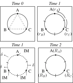
The economy lasts for three periods: (i) In the first period, banks form relationship links between them. (ii) Given the network formed, in the second period banks compete for deposits choosing deposit interest rates(rA, rB, rC). Fixed the rates, depositors must choose in which
bank they will deposit their good based on their expected payoff. Deposits raised by bankiare invested in a technology with random returnR˜iand meanR¯. In the end of the second period, after
investments are made, a fractionδof depositors will want to withdraw for early consumption.1
The bank will borrow from the interbank market to pay them and keep the investment intact. (iii) In the final period the return of the investments is realized and the game ends. The timing is illustrated by Figure 1. Each step of the model will be better described in the next paragraphs.
Figura 1 – Timing
Time 0
A
C B
Time 1
A(rA)
C (rC)
B (rB)
Time 1
A
C B
δ
δ δ
IM
IM IM
Time 2
A(RA)
C (RC)
B (RB)
Time 0:In the initial period, banks choose if they want to form links. Formally, a network
is a pairg = (b,[vij]|b|×|b|). The first element is a set of nodesb and the second element is a
1 The fraction of withdraws translate liquidity problems that banks can face during investment and insure the
matrix ([vij]|b|×|b|)) that translates the links formed. Nodes are banks,b ={A, B, C}, while for
the links we havevij = 1if banksiandj have a relationship andvij = 0otherwise. Links have
three effects on the model.2
First, for each link formed, banks’ investment become safer (in a mean-preserving-contraction sense). This effect is related to monitoring activities that interbank relation produces, specially interbank loans (Rochet and Tirole, 1996). Formally, for a given networkg, letg′ =
(b,[v′
ij]|b|×|b|)s.t.∃!(i, j)∈ {1, ...,|b|}2, vi,j −v′i,j <0. Assuming thatR˜i,g has a cdfFi(·, g)and
support[Rmin, Rmax], we state that:
|b| X
k=1
vik =
|b| X
k=1
vjk ⇒R˜i,g d
= ˜Rj,g
and
Fi(·;g′) so
Fi(·;g)
withE[ ˜R|g] =E[ ˜R|g′].3
Second, links reduce the liquidity costs that banks faces in the interbank market. Assu-ming that bankipays a spreadsi(g)for using the interbank market, we impose that:
si(g)> si(g′).
Third, links between neighbors banks reduce product differentiation. This effect comes from a standardization of banks’ services and attitudes after a long-term relationship between them. Following Matutes and Padilla (1994), in terms of the model, links reduce the transportation cost of depositors that are located in the neighborhood between the connected banks. The transportation cost refers to differences in preferences that depositors have for the heterogeneous products that are offer. Changes in the transportation cost allow us to explore the impact of changes in the degree of banks’ product differentiation. For a given networkg, a depositor of
bankithat is in neighborhoodijand isxdistant fromihas a transportation costx.tij(g)with:
tij(g) =
(
t, ifvij = 0
a.t, ifvij 6= 0, a∈(0,1).
The transportation cost represents a way to split the surplus generated by the investment between banks and depositors. Therefore,tij(g)can be seen as the degree of competition between
2 In this version of the paper we omit possible flows of resources that can happen between two competing banks
through the links formed. Doing so, we abstract from contagion effects. This not only makes the mathematical part more tractable, but highlights the channels between competition and network structure in a business-as-usual environment, when contagion problems seems unlikely or when an outside regulator credibly assures that contagion will not happen. Therefore, even though competing banks take part in the interbank market, there is no flow of resources between them.
3 The term d
iandj in the deposit market, for a given networkg. Since it is common to all banks, the termt
can be seen as the general level of competition in the market. While, since it only appears for linked banks and reduce the transportation cost, the termacapture the substitution effect that
comes out from the relationship between two financial institutions.
Time 1: In the second period banks compete for deposits choosing simultaneously
deposits’ interest rates,{rA, rB, rC}. After that, depositors will choose the bank that leaves him
with the highest expected payoff, taking into account an outside optionv - that can be easily
interpret as the utility of the depositor for keeping the good - and the transportation cost. Banks invest all the gathered deposits in the investment technology. In the end of the second period a fractionδof depositors from each bank wants to withdraw. To keep its investment intact, banks
must take a loan in the interbank market for paying those withdraws.4
We follow Matutes and Vives (2000) and assume limited liability with a standard debt contract for deposits and interbank debts. Bank i setting a deposit interest rate ri declares
bankruptcy when revenues cannot cover payment obligations:
˜
Ri,g <(1−δ)ri+δ(1 +si(g)).
If the bank cannot fulfill its commitments, creditors receive whatever funds left. We assume here that interbank debts have seniority in the payment in case of a bankruptcy. Therefore, for banki
to starts defaulting on interbank debts the investment return must be:
˜
Ri,g < δ(1 +si(g)).
Formally, for a given networkg, the amount a depositor of bankiexpect to gain from his deposit is:
φi(ri, si(g), g) = δ+pφi(1−δ)ri +
Z (1−δ)ri+δ(1+si(g))
δ(si+1)
[ ˜R−δ(si+ 1)]dFi( ˜R, g), (2.1)
wherepφi := 1−Fi((1−δ)ri+δ(si+ 1), g)is the probability of success of banki.5The first
term in the right side of equation (2.1) is the amount that depositor gather if it withdraw in period 1, times the probability of being a withdrawer. The second term is the amount collected when the depositor do not withdraw, the bankisets an interest rateri and the institution do not go
bankrupt. Finally, the third term is the expected gain for depositor from a liquidation of the bank. Therefore, taking into account the transportation and the opportunity cost, the expected payoff of depositor in bankithat isxdistant from it will be:
φi(ri, si(g), g)−x.tij(g)−v.
4 There is a shortcut in here. We could have think of a storage asset and let the bank invest in it for paying the
withdraws. Instead, we are going to assume that the cost of the bank to go for the interbank market is lower enough so we can use Allen and Gale (2000b) result, that is better for banks to invest all it gather from depositors and appeal for the interbank market if someone withdraw, rather then invest a fraction in the storage asset and suffer the opportunity cost of the expected long-term return.
5 We are assuming here that, when choosing a bank, depositor do not know if it want to consume in period one or
The expected cost of bankiwith the interbank by unit of deposit can be written as:
ψi(si(g), g) =pψi δsi +
Z δ(si+1)
Rmin
( ˜R−δ)dFi( ˜R, g), (2.2)
wherepψi :=
RRmax
δ (si(g) + 1)dFi( ˜R, g)is the probability that bankipays the interbank market.
The first term on the right side of (2.2) is the net payment for the interbank in case of bankihave
enough resources, while the second term is the expected payment for the interbank in case of a liquidation. Finally, assuming that bankiset a deposit interest rateri, its expected profit by unit
of deposit will be:
mi(ri, si(g), g) =
Z Rmax
(1−δ)ri+δ(si(g)+1)
( ˜R−δ(si+ 1)−(1−δ)ri)dFi( ˜R, g). (2.3)
Hence, we can write bankiprofit as:
Π =mi.(Mi,j+Mi,k)
whereMi,j is the market-share ofiin the neighborhoodij.
Time 2:Finally, in t = 3 the game is ended, with investment returns happening and banks going or not bankrupt.
To make the exposition clear and to separate the choice of the network from the rest of the game, we name the start of the second period to beyond as the competition subgame. Moreover, to keep the mathematical part tractable we make some complementary assumptions for our model:
1. F(·;g)is continuously differentiable andR˜has a support[0,∞);
2. the net effect of adding a link on the expected interbank market’s cost is negative, i.e.,
ψi(si(g), g)> ψi(si(g′), g′), ∀i∈b
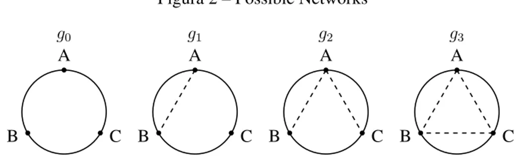
Note that, for the three banks case, all possible networks that can come out in equilibrium are: the no-links networkg0, the one-link networkg1, the two-links networkg2 and the all-links
networkg3. They are all illustrated in Figure 2. Any other network is only a permutation of
index from these four. It is noteworthy that in all results presented we are not taking into account equilibria that are only an index permutation of others. If we prove for one set of index, a permutation of them is trivially an equilibrium.
2.1
Equilibrium
Figura 2 – Possible Networks
g0
A
C B
g1
A
C B
g2
A
C B
g3
A
C B
Definition 2.1.1(Bernheim et al, 1987). An agreement is self-enforcing if and only if no proper subset (coalition) of players, taking the actions of its complement as fixed, can agree to deviate in a way that makes all of its members better off.
Definition 2.1.2(Bernheim et al, 1987). An agreement is coalition-proof if and only if it is Pareto efficient within the class of self-enforcing agreements
The characteristic of coalition-proof definition refine the one of Nash equilibrium in a way that not only individual deviations must be excluded from a possible equilibrium strategy, but also deviations of a group of players. If we see links as an agreement between players, we can naturally apply the definition of coalition-proof to networks. Now, we are able to define an equilibrium for our game:
Definition 2.1.3. A pair(g,{ri}i∈b)is an equilibrium of the game if
• giveng,{ri}i∈bis a pure-strategy Nash equilibrium of the competition subgame;
• the networkg is coalition-proof.
To avoid uninterested cases like local monopoly, we present results only for equilibria where, given the interest rates charged, no bank is taken out of the market and there is no unattended depositor, i.e.:
• ∀i, j ∈b, 0< Mi,j <1;
• all marginal consumers derives a non-negative surplus.
We refer to these as the direct competition conditions (DCC). We refine our definition of equilibrium to take into account those restrictions:
Definition 2.1.4. A pair(g,{ri}i∈b)is an interior equilibrium of the game if
• (g,{ri}i∈b)is an equilibrium of the game;
3 Competition Subgame
Using the backward induction method, we start by solving the competition subgame for a given network.1For a set{r
i}i∈b that satisfy the direct competition conditions, the marginal
depositor in neighborhoodij with distancenij of bank i has a payoff:
φi(ri, si)−tijnij −v =φj(rj)−(1−nij)tij−v
⇐⇒ nij =
φi(ri)−φj(rj)
2tij
+ 1/2.
It is easy to see that, in a DCC scenario, the distance of the marginal depositor from the bank is always equal to the bank’s market-share on the neighborhood. Hence, for a given set of deposit interest rate{rj, rk}fixed by others, bankibest response is:
{ri∗}=argmax ri
mi(ri, si).
φi(ri)−φj(rj)
2tij
+ φi(ri)−φk(rk) 2tik
+ 1
.
Using the definition of marginm, depositor expected gainφand expected cost in the interbank
marketψ, we can come to an identity:
mi+φi+ψi = ¯R, ∀i∈b.
This only states that all resources generate by the investment must be distributed between banks, depositors and interbank market. Therefore, we can rewrite bankiproblem as:
{ri∗}=argmax ri
{( ¯R−ψi(si)−φi(ri, si)).(ni,j+ni,k)}. (3.1)
As a first result, we prove that for any network a best response for a bank always exists and is unique.
Lemma 3.0.1. For a given networkg ∈ {g0, g1, g2, g3}, a competition subgame pure strategy
Nash equilibrium exists and is unique.
Hence, with{ri}i∈b attending for the direct competition conditions, we have a unique
expression for banks’ best response on deposit interest rate. Below we describe and discuss the solution of the competition subgame for each possible network. We came to a general result for a genericg, but since it is not intuitive to present it in an extensive form, we opt for showing the
result separately by networks. After each competition scenario we follow with the parameters’ inequalities that express the direct competition conditions.
1 From now own, to make the exposition clear, we suppress the termgfrom the functions when we deal with a
3.1
Symmetric Network
LetgS ∈ {g0, g3}as showed in Graph 2. Solving (3.1) for this structure, we can come to
a simple solution for banks margin and market-share.
Lemma 3.1.1. For a given networkgS, supposing that DCC holds, the set{rA, rB, rC}is a Nash
Equilibrium of the competition subgame if and only if
mi =tij(gS)
for alli∈b. Which impliesnij = 21 for any pair(i, j)∈b×b.
This result is analogous to the original one from Salop (1979). As tij falls, demand
becomes more elastic and prices (that can be seen as−φ(ri, si)) move toward marginal cost.
Thus, the termtij is the relevant measure of monopolistic product differentiation in the model.
Note that, in a game where there is no flow through links, the complete networkg3does
not create any differentiation between banks and only increases the substitutability for everyone. Hence, banks always want to deviate fromg3 back tog0. In addition, it is noteworthy the fact that
the investment return does not appear in banks’ best-response margin. Since we are dealing with a direct competition case, any increase in the expected return is translated into a higher deposit interest rate, so that banks would not lose market-share for the neighbor.
By symmetry, market-shares are the same for any set of parameters. Therefore, we only need to worry with the DCC of a non-negative surplus for the marginal depositor. For a given banki,
¯
R−ψi(si)≥
3
2tij(g) +v
This condition states that the mean return must be large enough so that banks can be capable of offering an interest rate that covers the costs of any depositor in near neighborhoods and still have positive margins. If this condition is not attended, banks will have monopoly regions and depositors in the middle of the neighborhoods will opt for the outside option.
3.2
Asymmetric Networks
In this section we have two cases to deal with. The one that only two banks are connected (g1) and the one that only one bank is connected to two others (g2). In both cases, since the model
has three players, we only need to separate the response of the most connected bank from the response of the least connected one.
First we present the result for an asymmetric network g1, where only A and B are
connected. LetK :=ψC(sC)−ψA(sA)be the difference of expected liquidity costs between
Lemma 3.2.1. For the networkg1, assuming DCC holds, the set{rA, rB, rC}is a Nash
Equili-brium of the competition subgame if and only if
mB =mA =
5a
3a+ 2t+
a
3a+ 2K
mC =
4a+ 1 3a+ 2t−
a+ 1 3a+ 2K.
Which impliesnAB = 1/2andnBC =nAC = 2(32aa+3+2) + 2(3a+1a+2)Kt.
Now, margins depend not only on the substitution effect, but also on the difference of liquidity costs. The link made between A and B clearly becomes an advantage in the competition for depositors in terms of cost reduction. A higher difference in what banks expected to pay for the interbank market (K) affects positively both margin and market-share of the ones with more relationships. Moreover, the substitution effect (a) has an important role on the best response. The parameteraintensifies the competition in the neighborhood between the two linked banks. It can be strong enough to compensate all the gains from the difference of liquidity costs in margin and make banks unwilling to form the link. Therefore, excluding the demand elasticity (t) that appears also in the symmetric network case, we have two main forces acting here. A
positive incentive for banks to connect because of the gains over the difference in liquidity costs. A negative effect in the willingness of making links with neighbors due to the substitution effect, that can come out of practices’ standardization in the interbank relationship.
The DCC inequalities for this case are the following:
t ≥ a+ 1
4a+ 1K (3.2)
¯
R−ψ(sA)≥
3(4 +a)a
2(3a+ 2)t+v +
a
3a+ 2K (3.3)
¯
R−ψ(sC)≥
3(4a+ 1)
2(3a+ 2)t+v−
3(1 +a)
2(3a+ 2)K (3.4)
Inequality (3.2) refer to market-shares in neighborhoods AC and BC. It guarantees that the asymmetry of liquidity costs is not too large so that A and B could exclude C from the market and still set positive margins. Note that, the lower the substitution effect becomes (highera), the
higher the difference in liquidity cost must be for A and B to exclude C from the market. This happens because the market-share of the connected banks is increasing on the substitution effect. If competition intranet is intense, banks must set lower margins for not loosing too much share against their peer. But, lower margins make connected players to gain share outside the network. With high market-shares, it is only needed a small advantage in costs to exclude not connected banks from the market.
case, except for the liquidity cost difference. Those inequalities make clear the difference in competition in each neighborhood that comes out of the asymmetric case. In neighborhood AB banks must have an expected return high enough to compensate the gains from lower spreads that others have and so be able to compete direct with them. While in neighborhoods AC and BC, the fact that one competitor has an advantage over the other, makes possible for them to set lower margins and still compete directly.
Next, we present the result for an asymmetric networkg2, where bank A is connected to
B and C, but B and C are not.
Lemma 3.2.2. For a giveng2, assuming DCC holds, the set{rA, rB, rC}is a Nash Equilibrium
of the competition subgame if and only if
mA=
a(4 +a) 2a+ 3 t+
4a+ 5 4(2a+ 3)K
mB =mC =
5a
2a+ 3t− 1 2a+ 3K.
Which impliesnBC = 1/2andnAC =nAB = 2(2a+4a+3) + 2a(2a+1a+3)Kt
In this network structure, the two forces that where playing ing1 are still valid. A higher
difference in liquidity cost (higherK) implies a higher margin and share for the most connected. A higher substitution effect (lowera) implies a lower margin set by bank A. However, now the most connected bank has a lower bound for the second force that is different from zero. Even if the substitution effect increases substantially (a → 0), the most connected bank can keep positive margin and market-share simply because it has a liquidity cost lower than the others. We will prove in the next section that, in this network, profits of the most connected bank will always be higher than the others.
For this case, direct competition conditions are similar to the ones fromg1 case, with
4 Solving the Model
Substituting the results found in the lemmas above, we can rewrite banks’ expected profits as a function of only three exogenous parameters:t,aandK. To differentiate the networks and institutions, we denote profits byΠwith a lower index for each possible network and an upper index for differences in the number of links, withhfor the most connected andlfor the least
connected agent.
Πg0 =t Πg3 =a.t
Πh g1 =
a(a+1)[K+5t]2
2t(3a+2)2 Πhg 2 =
[K(1+a)+at(4+a)]2
at(2a+3)2
Πl g1 =
[t(1+4a)−K(1+a)]2
t(3a+2)2 Πlg 2 =
(a+1)[5at−K]2
2at(2a+3)2
To compute non trivial equilibria, we are going to eliminate the cases where the substitu-tion effect is so strong that any link become a competisubstitu-tion disadvantage for banks. If we set a lower bound of2/7for the substitution effecta, then DCC is a sufficient condition to eliminate
this extreme cases, i.e., if the effect of a relationship is harmful for the bank, we must already be in a situation of monopoly or entrance elimination.
Lemma 4.0.3. For a given(a, K, t)∈(2/7,1)×R++×R++, if(a, K, t)attends DCC for any
network, then:
Πh
g2 >Πlg2 andΠhg1 >Πlg1.
Since post-network play is uniquely determined, we may replace the subgame with the associated continuation payoff to produce a static network game between banks.1A Coalition-Proof Nash Equilibrium2of this new static game is an interior equilibrium of the original one. Evaluating the possibility of deviations in this new game, we can come up with four thresholds that define regions in the competition level space that fully characterize the game equilibrium.
Proposition 4.0.4. For a given(a, K)∈(0.36,1)×R++, an interior equilibrium in the game
is completely characterized by four thresholds in the competition dimension.
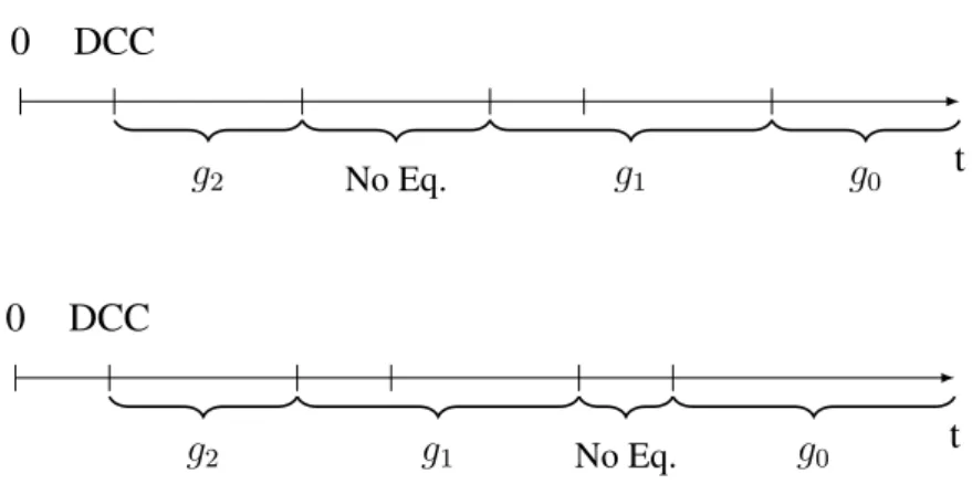
In Figure 3 we present two possible positions for the thresholds, that are driven by different values ofaandK. Note that the region of interior equilibrium can only be characterized
after the DCC is attended. Moreover, different values ofaandK can result in different orders between thresholds. Finally, note that this fully characterization only holds for values ofagreater
then0.36, i.e., the substitution effect can not be too large. This comes out to ensure that banks will be able to make any relationship and still attend DCC, as can be seen in the proof of the proposition.
Figura 3 – Possible equilibrium determinations 0 DCC
t
g0
g1
No Eq. g2
0 DCC
t
g0
No Eq. g1
g2
Moreover, when we compute the thresholds and evaluate limits foraandK we have a
similar result to that found by Matutes and Padilla (1994). For a fixed level of competitiont, we can always find a value forK oralarge enough so that the no-link network do not come out in equilibrium. But, the possibility of no pure strategy equilibrium in our environment does not allow us to state that we can always find parameters for a partial network to come out in equilibrium.
The corollary we present below is the main result of the monopolistic competition environment. It comes out directly from the determination of equilibrium through thresholds. It states not only that, in this framework, competition is a major element in the determination of the interbank network structure, but also that the effect has a unique direction. As a consequence of the model, in a monopolistic environment more competition is related to a denser relationship network between banks.
Corolary 4.0.5. For a given(a, K)∈(0.36,1)×R, in direct competition conditions the density of the network is increasing on the competition level.
4.1
Collusion
Proposition 4.1.1. Leta∈(0.5,1)and assume thatR¯ ≥ψ(s(g3), g3) +at2 +v.3If banks get into
a collusion for deposits that attends DCC, then the networkg3always come out in equilibrium.
In a collusion environment there is no gains in volume when banks have differences in the interest rates set. Transfers for depositors through interest rates imply only a reduction in margin. Therefore, banks want to set rates small enough so to extract all surplus from the marginal depositor, taking into account a participation constraint. Note that links reduce both the transportation and the expected interbank cost. Hence, denser networks imply large profits for all. The result here inverts the one from the monopolistic competition case. The effect of competition level becomes ambiguous when we take into account the possibility of collusion.
3 The conditionR¯ ≥ψ(s(g
3), g3) + at
2 +vonly assure that banks have a non-negative profit at least in network
5 Conclusion
In this paper we develop a framework to understand the interaction between competition and network formation decision in the banking market. From it we can conclude that the competition level exerts a key role in the construction of relationship networks between banks. This role comes from the effect that banks’ competitive conduct have on the network outcomes. In a monopolistic competition environment, the decision of making connections between banks has a trade-off between cost reductions and substitutability. The competition level affects the final choice of the bank to make a link, since it affects the importance of the elements in this trade-off. When the general competition is not too intense, the lost of margin in a fierce competition intra-network becomes a great sacrifice when comparing to the gains of lower liquidity cost in an inter-network competition. When banks are competing sharply for depositors, a bigger demand elasticity in the competition against their peers does not seem relevant for the bank, comparing with the advantages that the relationship will bring in the inter-network competition. Therefore, different network topologies come out of different competition levels and greater competition imply denser networks.
The possibility of collusion between banks alter drastically that trade-off. When there is a concerted strategy, the effect of margin reduction that comes out of substitution effect is vanished. The gains from standardizing products are completely internalized by the banks. Therefore, in this new competition environment, links exert only positive effects of costs reduction. As a direct consequence, only the densest network comes out in equilibrium. When we allow for the possibility of collusion, the effect of competition on the network topology becomes ambiguous.
The model we build made possible to find aspects of interbank relationships and competi-tion that give rise to four different network topologies. Since, by definicompeti-tion, a link between banks imply less risk investments, in our model a denser network is also more stable.1Therefore, in a monopolistic competition environment, more competition is related to a more stable financial system. But, note that we are not taking into account contagion effects. Therefore, we are at some point overstating the likelihood of networks with connections. An important step for the research is to incorporate effects of contagion on banks’ decision to form links in different competition scenarios.
In addition of the contagion aspects already mentioned, another path for our research is an empirical analyses of the relations that where presented in this work. Most importantly, to look for a possible identification strategy that isolates the relation competition-network topology from other determinants. The major barrier for this kind of analysis relies in the privacy of interbank relationship data. In the best of our knowledge, there is no empirical work in banking that deal
1 We borrow from Acemoglu, Ozdaglar and Tahbaz-Salehi (2013) the term stable. For the authors, the stability of
References
ACEMOGLU, D.; OZDAGLAR, A.; TAHBAZ-SALEHI, A. NBER WORKING PAPER SERIES SYSTEMIC RISK AND STABILITY IN FINANCIAL NETWORKS Systemic Risk and Stability in Financial Networks.NBER working papers series, n. January, 2013. ISSN
1098-6596.
AFONSO, G.; KOVNER, A.; SCHOAR, A. Trading Partners in the Interbank Lending Market.
Working Paper, n. October, p. 0–53, 2014.
ALLEN, F.; GALE, D.Comparing financial systems. MA: MIT Press, 2000. 419 p. ISSN
08981221. ISBN 0893-9454.
ALLEN, F.; GALE, D. Financial Contagion.The Journal of Political Economy, v. 108, n. 1, p.
1–33, 2000. ISSN 00223808.
ALLEN, F.; GALE, D. Competition and Financial Stability.Journal of Money, Credit, and Banking, v. 36, n. 3, p. 453–480, 2004. ISSN 1538-4616.
BERNHEIM, B. D.; WHINSTON, M. D. Coalition-Proof Nash Equilibria I . Concepts.Journal of Economic Theory, v. 42, p. 1–12, 1987.
BLUME, L. et al. Network formation in the presence of contagious risk. In:12th ACM Conference on Eletronic Commerce. [S.l.: s.n.], 2011.
BOYD, J.; NICOLO, G. D. The theory of bank risk taking and competition revisited.The Journal of finance, v. 60, n. 3, p. 1329–1343, 2005.
BOYD, J. H.; NICOLÓ, G. D.; SMITH, B. D. Crises in Competitive versus Monopolistic Banking Systems.Journal of Money, Credit and Banking, v. 36, n. 3, p. 487–506, 2004.
CALOMIRIS, C. W.; KAHN, C. M. The Efficiency of Self-Regulated Payments Systems: Learning from the Suffolk System.Journal of Money, Credit and Banking, v. 28, n. 4, p.
766–797, 1996.
CARLETTI, E. Competition and Regulation in Banking. In: THAKOR, A.; BOOT, A. (Ed.).
Handbook of Financial Intermediation and Banking. [S.l.]: Elsevier, 2008.
CARLETTI, E.; HARTMANN, P.; SPAGNOLO, G. Bank Mergers, Competition, and Liquidity.
Journal of Money, Credit and Banking, v. 39, n. 5, p. 1067–1105, aug 2007. ISSN 0022-2879.
CARLETTI, E.; LEONELLO, A. Credit Market Competition and Liquidity Crises. 2014. COCCO, J. F.; GOMES, F. J.; MARTINS, N. C. Lending relationships in the interbank market.
Journal of Financial Intermediation, Elsevier Inc., v. 18, n. 1, p. 24–48, jan 2009. ISSN
10429573.
DIAMOND, D.; DYBVIG, P.Bank Run, Deposit Insurance, and Liquidity. 1983. 401–419 p.
FREIXAS, X.; PARIGI, B.; ROCHET, J. Systemic risk, interbank relations, and liquidity provision by the central bank.Journal of money, credit and banking, v. 32, n. 3, p. 611–638,
2000.
GOLDSTEIN, I.; PAUZNER, A. Demand-deposit contracts and the probability of bank runs.
Journal of Finance, v. 60, n. 3, p. 1293–1327, 2005. ISSN 00221082.
HELLMANN, T.; MURDOCK, K.; STIGLITZ, J. Liberalization, moral hazard in banking, and prudential regulation: Are capital requirements enough?American economic review, v. 90, n. 1,
p. 147–165, 2000.
KEELEY, M. Deposit insurance, risk, and market power in banking.The American Economic Review, v. 80, n. 5, p. 1183–1200, 1990.
KNITTEL, C. R.; STANGO, V. Strategic incompatibility in ATM markets.Journal of Banking and Finance, Elsevier B.V., v. 35, n. 10, p. 2627–2636, 2011. ISSN 03784266.
MARTINEZ-MIERA, D.; REPULLO, R. Does competition reduce the risk of bank failure?
Review of Financial Studies, n. 0801, 2010.
MATUTES, C.; PADILLA, A. Shared ATM networks and banking competition.European Economic Review, v. 38, n. 5, p. 1113–1138, 1994. ISSN 00142921.
MATUTES, C.; VIVES, X. Imperfect competition, risk taking, and regulation in banking.
European Economic Review, v. 44, n. 1, p. 1–34, jan 2000. ISSN 00142921.
REPULLO, R. Capital requirements, market power, and risk-taking in banking.Journal of Financial Intermediation, v. 13, n. 2, p. 156–182, apr 2004. ISSN 10429573.
ROCHET, J.; TIROLE, J. Interbank lending and systemic risk.Journal of Money, credit and Banking, v. 28, n. 4, p. 733–762, 1996.
ROCHET, J.-C.; VIVES, X. Coordination Failures and the Lender of Last Resort: Was Bagehot Right After All?Journal of the European Economic Association, v. 2, n. December, p. pp.
1116–1147, 2004. ISSN 15424766.
SALOP, S. Monopolistic competition with outside goods.The Bell Journal of Economics, v. 10,
n. 1, p. 141–156, 1979.
APPENDIX A – Proofs
Demonstração. (Lemma 3.0.1) Fix g and a pair (r∗
j, r∗k). Note that φ′(x) = pφ(x)(1 −δ) >
0,∀x∈R+ ⇒φis an injection fromR+toR+.
Letf :Im(φ)→Rs.t.
f(x) = ( ¯R−x−ψ(si))(
x−φ(rj)
2tij
+x−φ(rk) 2tik
+ 1)
Rewritef as:
f(x) =−x2T
2 +x(
m
2.T −C) +m.C
where T = 1 tij +
1
tik, m = ¯R −ψi(si)and C = − φ(rj)
2tij − φ(rk)
2tik + 1 It is easy to see thatf
is a strictly concave function ⇒ ∃!x∗ ∈ Im(φ) s.t. x∗ ∈ argmaxf. Finally, φ an injection
⇒ ∃!r∗ ∈R
+s.t.φ(r∗) =x∗.
In the proof below we solve for a generic networkg. Lemma 3.1.1, 3.2.1 and 3.2.2 comes out by the substitution of the transport cost.
Demonstração. (Lemma 3.1.1, 3.2.1 and 3.2.2) For a given pair networkg and a pair(r∗
j, rk∗),
supposing that DCC holds, we can use the definition of the marginal consumer to write banki
problem as:
max
ri {( ¯R−φ(ri)−ψ(si))(
φ(ri)−φ(rj)
2tij(g)
+φ(ri)−φ(rk) 2tik(g)
+ 1)
By lemma 3.0.1 a solution exist and is unique. The first order condition is such that:
φ(ri∗) =
¯
R−ψ(si)
2 +
tik
tij +tik
φ(r∗
j)
2 +
tij
tij +tik
φ(r∗
k)
2 −
tijtik
tij +tik
Let A ≡ [aij]3x3 s.t. aii = 0 and aij = (tik/(tij +tik)), and C ≡ [ci]3x1 s.t. ci =
(tij.tik)/(tij+tik)we can solve for the vector of best responses using:
ˆ
φ = (I−0.5A)−1(0.5 ˆR−C)
whereRˆ = [ ¯R −ψi(si)]3×1. It is easy to see that an inverse of(I −A)exist for any
Demonstração. (Lemma 4.0.3) Fix (a, K, t) ∈ (2/7,1)×R++×R++. Using the subgame
profits solution, definefg1 := Π
h g1 −Π
l
g1 andfg2 := Π
h g2 −Π
l
g2. For a giventwe have:
fg1(t) =
(−7a2+ 9a−2)t2+K(26a2+ 30a+ 4)t−K2(a2+ 3a+ 2)
(18a2+ 24a+ 8)t
fg2(t) =
a2(2a2−9a+ 7)t2+Ka(4a2+ 30a+ 26)t+K2(2a2+ 3a+ 1)
a(8a2 + 24a+ 18)t
Note that, sincet >0anda∈(0,1), the signals and roots offg1 andfg2 are completely charac-terized by the second order polynomial in the numerator. Lethg1 andhg2 be those numerators for the respective networks.
• (a, K) ∈ (2/7,1) × R++ ⇒ hg1(0) < 0andh
′′
g1(t) > 0,∀t ∈ R++ ⇒ ∃!t
g1
hl >
0s.t.hg1(t)>0,∀t ≥t
g1
hl,⇒fg1(t)>0,∀t≥t
g1
hl
• (a, K)∈(0,1)×R++ ⇒hg2(0)>0andh
′′
g2(t)>0,∀t∈R++. Sinceargmint{hg2}<
0,∀(a, K)∈(0,1)×R++, thenhg2(t)>0,∀t >0⇒fg2(t)>0,∀t >0. Letthl =tg
1
hl. Solvinghg1(t) = 0, we have:
thl =
13K
7 +
3K((2a(a+ 1))(1/2) + 2)
a−1 −
12K(7(2a(a+ 1))(1/2) + 6)
7(7a−2) >0,
∀(a, K)∈(1/7,1)×R++
Finally, we know that(a, K, t)attends DCC for anyg ⇒t≥ (a4+1)a+1K =:z. It is easy to see thatz ≥thl,∀(a, K)∈(2/7,1)×R++.
Demonstração. (Proposition 4.0.4) Fix(a, K)∈(0.36,1)×R++. Lett ∈R++such that DCC
holds.
Since DCC holds, for each possible network there is a unique solution for the competition subgame. Hence, we may replace the subgame with the associated continuation payoff to produce a static network game. Deviations between the four possible networks can be fully characterize by differences in profits:
Deviation Difference
g0 tog1 ⇐⇒ Πhg1(t)>Πg0(t) (1)
g0 tog2 ⇐⇒ Πhg2(t)>Πg0(t)andΠ
l
g2(t)>Πg0(t) (2)
g0 tog3 ⇐⇒ Πg3(t)>Πg0(t) (6)
g1 tog2 ⇐⇒ Πhg2(t)>Π
h
g1(t)andΠ
l
g2(t)>Π
l
g1(t) (3)
g1 tog3 ⇐⇒ Πg3(t)>Π
h
g1(t)andΠg3(t)>Π
l
g1(t) (4)
g2 tog3 ⇐⇒ Πg3(t)>Π
l
Note that this relation is antisymmetric, i.e., if there is no deviation fromgxtogy, then
banks will deviate fromgy togx. We assume here that if profits are equal, banks prefer not to
make the link.
Using lemma 4.0.3 and the fact thatΠg3 <Πg0 always hold, some simplifications can be made:
• tattend DCC⇒(2) resume toΠl
g2(t)>Πg0(t)and (4) toΠg3(t)>Π
h g1(t).
• (1) and not(6)⇒not(4) • (5) and not(6)⇒not(2)
Therefore, we can characterize pure strategy equilibria by only 3 main differences:
Conditions Equilibrium
not(1) and not(2) ⇒ g0
(1) and not(3) ⇒ g1
(3) and (2) ⇒ g2
(1) and (3) and not(2) ⇒ No equilibrium (2) and not(1) and not(3) ⇒ No equilibrium
Since conditions are inequalities, we only need to find the thresholds in the space of competition level (t) that rule where conditions are valid or not.
Let f1 := Πhg1 −Πg0,f2 := Π
h
g2 −Πg0,f3 := Π
h g2 −Π
h
g1 andf4 := Π
l g2 −Π
l
g1. In an extensive form:
f1(t) =
(7a2
+a−8)t2
+ (10a2
+ 10a)tK+ (a2
+a)K2
(18a2+ 24
a+ 8)t
f2(t) =
(a4
+ 4a3
+ 4a2
−9a)t2
+ (2a3
+ 10a2
+ 8a)tK+ (a2
+ 2a+ 1)K2
(4a3+ 12
a2+ 9
a)t
f3(t) =
(18a6
+ 68a5
+ 88a4
−77a3
−97a2
)t2
+ (−4a5
+ 68a4
+ 190a3
+ 182a2
+ 64a)Kt
(72a5+ 312
a4+ 482
a3+ 312
a2+ 72
a)t
+(−4a
5
+ 2a4
+ 39a3
+ 65a2
+ 40a+ 8)K2
(72a5+ 312
a4+ 482
a3+ 312
a2+ 72
a)t
f4(t) =
(97a5
+ 77a4
−88a3
−68a2
−18a)t2
+ (64a5
+ 182a4
+ 190a3
+ 68a2
−4a)Kt
(72a5+ 312
a4+ 482
a3+ 312
a2+ 72
a)t
+(−8a
5
−40a4
−65a3
−39a2
−2a+ 4)K2
(72a5+ 312
a4+ 482
a3+ 312
a2+ 72
a)t
Note that, in all functions the signal and roots are fully determined by the second order polynomial in the numerator. Leth1,h2,h3 andh4 the numerator of each respective function.
The existence of thresholds comes from the fact that:
a ∈(0,1)∧K >0⇒
h1(0) >0∧h′′1 <0 ⇒ ∃!t1 >0 s.t. f1(t)<0,∀t > t1
h2(0) >0∧h′′2 <0 ⇒ ∃!t2 >0 s.t. f2(t)<0,∀t > t2
a∈(0.36,1)∧K >0⇒h′′4 <0, h4(0)<0, argmin{h4}>0and min{h4}>0⇒
∃!{tmin4 , t4} s.t. f4(t)<0,∀t /∈(tmin4 , t4)
Finally, we only need to prove that thresholds attends the DCC. Since we can always increase R¯ to guarantee that marginal depositors have non-negative expected payoff, DCC
conditions resume to:
t≥ (a+ 1)K 4a+ 1 >
(a+ 1)K
(3a+ 2)a
Substituting the DCC limitDCC¯ = (a+1)K
4a+1 in the second order polynomials, we have
∀(a, K)∈(0.36,1)×R++:
h1( ¯DCC)>0, h2( ¯DCC)>0, h3( ¯DCC)>0andh4( ¯DCC)>0⇒
t1, t2, t3andt4 attends DCC, buttmin4 do not.
Therefore, for a generic(a, K)∈(0.36,1)×R++, the regions defined byt1, t2, t3 and
t4fully characterized the network that comes out in an interior equilibrium.
Demonstração. (Corollary 4.0.5) For a given(a, K)∈(0.36,1)×R++, lett, t′ andt′′s.t. DCC
holds for all and:
• for(a, K, t),g0 comes out in equilibrium;
• for(a, K, t′),g
1comes out in equilibrium;
• for(a, K, t′′),g
2 comes out in equilibrium.
If we prove thatt > t′ > t′′we are done. Using the proof of proposition 4.0.4, we know:
g0 interior equilibrium⇒t > t1∧t > t2
g1 interior equilibrium⇒t1 ≥t′ ∧(t′ ≥t3∨t′ > t4)
g2interior equilibrium⇒t2 ≥t′′∧t3 ≥t′′∧t4 ≥t′′
Demonstração. (Proposition 4.1.1)
Fix(a, t) ∈ (0.5,1)×R++and assume R¯ ≥ ψ(s(g3), g3) + at2 +v holds. For a given
networkg, if banks get into a collusion for deposits respecting DCC, then they solve the problem.
max
{rA,rB,rC}
{3 ¯R−X
i∈b
(φ(ri) +ψ(si))(
φ(ri)−φ(rj)
2tij
+φ(ri)−φ(rk) 2tik
+ 1)} s.t.
φ(ri)−(
φ(ri)−φ(rj)
2tij
+1
2)tij −v ≥0, ∀i, j ∈b, i 6=j (A.1)
1> φ(ri)−φ(rj)
2tij
>0 (A.2)
Let{r∗
A, rB∗, rC∗}a solution for the problem. Since (2) holds, it is easy to see that (1) must
be biding in the solution. Solving the system φ(r∗i)+φ(r∗j)
2 =v+
tij
2 ,∀i, j ∈b, i6=j, we have:
φ(ri∗) =
tij
2 +
tik
2 −
tjk
2 +v,∀i∈b (A.3)
Note that, fora >1/2this solution attend condition (2) for any network. Substituting (3) in the profits’ sum function and diving the amount equally between the players we come to an individual profit for each possible network:
Πg3 = ¯R−ψ(s(g3), g3)−
at
2 −v Πg0 = ¯R−ψ(s(g0), g0)−
t 2 −v
Πg1 = ¯R−(
a2
3 −
a
2 + 2
3)t−[(1−
a+ 1
3 )ψ(g1, sC(g1)) +
a+ 1
3 ψ(g1, sA(g1))]−v
Πg2 = ¯R−(
4a2−3a+ 2
6a )t−[
2−1/a
3 ψ(gA(g2), g2) + (1−
2−1/a
3 )ψ(gC(g2), g2)]−v
Note that:
• ψ(s(g3), g3)is strictly lower then any strict convex combination of interbank costs ing1
andg2
• a 2 <
4a2
−3a+2 6a <
a2
3 −
a 2 +
2
3 <1, ∀a∈(0.5,1)