A Credit Scoring Model for the Portuguese Private Clients
Daniela Nikaitow de OliveiraInternship report Master in Finance
Supervised by
Carlos Francisco Ferreira Alves
iii
Banco L. J. Carregosa, S.A.
This report was made in the context of a curricular internship done at Banco L. J. Carregosa, S.A., where I have worked since September 2017 until March 2018.
Banco L. J. Carregosa, S.A. is a Portuguese credit institution, specialized in the private banking, which main goal is to advise its clients and to protect its propriety. It was founded in the XIX century, more precisely in a financial home in 1833, for the negotiation of currencies. The bank was such a novelty at that time, that was even created 13 years before the foundation of Banco de Portugal. 52 years later, in 1885, it was acquired by Lourenço Joaquim Carregosa, to whom the bank owns its name and a reputation of credibility and trust that remains until today. At the end of the last century, the bank originated L. J. Carregosa – Sociedade Corretora S.A., that, later, was transformed into Sociedade Financeira de Corretagem and, finally, into Banco L. J. Carregosa, S.A. (Banco Carregosa).
Nowadays, Banco Carregosa is mainly recognized for allying tradition with modernity, for the creation and development of innovative financial products and for detaining an online business. In fact, in 2000, Banco Carregosa made available the first online brokerage service in Portugal that led, in 2007, to the creation of the GoBulling brand.
v
Biographical note
Daniela Nikaitow de Oliveira is a Portuguese girl, born in São Paulo (Brazil), in 1995, with Japanese ancestry.
In 2013, she moved from Carregal do Sal (Viseu) to Porto to enroll the BSc in Management at the School of Economics and Management of the University of Porto, which she completed in 2016.
At the same year, she enrolled in the Master in Finance program at the same institution; and, in 2017, she started a curricular internship at Banco L. J. Carregosa, S.A., which the present internship report explains the work developed and concludes the Master.
vii
Acknowledgments
I would like to thank- Carlos Francisco Alves, my professor and supervisor, for guiding me and helping me throughout this work, during the last several months;
- Mariana Lopes and Diamantino Leite, from Banco Carregosa’s Risk Department, for receiving me in their installations and proposing me an interesting topic of research;
- my parents, Rui and Sueli, for always believing in me and investing in my education and career, to whom I am forever grateful;
- my sisters, Fernanda and Carolina, for always incentivizing me during the 23 years of my life and for all the memories shared together;
ix
Abstract
Given the increase number of bankruptcies that happened in the last years, especially after the financial crisis, and the regulatory constraints imposed by the Basel Committee on Banking Supervision and the National and European Authorities, the concern regard credit risk has increased dramatically.
This study, developed in the context of an internship done at Banco L. J. Carregosa, S.A., aims at developing a credit scoring model to calculate the probability of default of private clients, having in mind the five C’s of credit: personal and socio-professional Characteristics; Character, Capital, Collateral and Cycle conditions. The data used to develop it was retrieved from a survey developed by the European Central Bank with conjunction with several countries of the Eurozone, entitled “Household Finance and Consumption Survey”, in 2013.
The research evidences that what seems to play a major role when evaluating credit scoring models is the value of the cut-off; and that it is better to regress a model individually for each country (instead of combining information of different countries and benefiting from a higher number of observations). The model proposed presents a total accuracy rate equal to 78.29% and better accuracy results than the probabilistic model developed by Henriques (2014) and the rating model developed by Saunders and Cornett (2012).
Key-words: Credit scoring model, credit risk, probabilistic model JEL-Codes: C51, D14, E51, G21
xi
Resumo
Tendo em consideração o aumento do número de falências que ocorreram nos últimos anos, especialmente após a crise financeira, e as mudanças em termos de regulação impostas pelo Comité da Basileia na Supervisão Financeira, pelos supervisores nacionais e Europeus, a preocupação em relação ao risco de crédito tem aumentado drasticamente.
Desta forma, este estudo, desenvolvido em contexto de estágio curricular realizado no Banco L.J. Carregosa, S.A., tem como objetivo o desenvolvimento de um modelo de crédito para aferir a probabilidade de incumprimento de clientes particulares, tendo em conta os cinco C’s do crédito: Características pessoais e socioprofissionais, Carácter, Capital, Colateral e Condições da economia. A informação utilizada para desenvolver o modelo foi retirada de um inquérito desenvolvido pelo Banco Central Europeu juntamente com diversos países da zona euro, em 2013, intitulado “Inquérito à Situação Financeira das Famílias” (ISFF).
Este estudo proporciona evidência de que o que causa maior impacto quando este é avaliado, é o cut-off escolhido. Para além disso, é importante fazer a regressão de um modelo usando informações individuais do país em causa, em vez de se usar informações de vários países, apenas para fazer proveito de um maior número de observações. O melhor modelo apresentado neste estudo apresenta uma taxa de acerto global igual a 78.29%, que são resultados melhores que os alcançados por Henriques (2014) e Saunders and Cornett (2012), no seu modelo de rating.
O modelo desenvolvido pode ser utilizado por qualquer instituição financeira, que beneficiará de um modelo único, desenvolvido com informação providenciada pelo Banco Central Europeu e pelo Instituto Nacional de Estatística.
xiii
List of Contents
Chapter 1: Introduction ... 1
Chapter 2: Literature Review ... 5
Part A. ... 5
1.1 Corporations vs. Retail Loans ... 5
1.2 Traditional Approaches to Credit Risk ... 6
1.2.1 Expert Systems ... 6
1.2.2 Rating Systems ... 7
1.2.3 Credit Scoring Models ... 9
1.3 BIS Basel New Capital Accord ... 13
Part B. ... 14
Chapter 3: Data Description & Methodology ... 19
Part A: The Survey ... 19
Part B: Methodology ... 20
Part C: Data Description ... 28
Chapter 4: The Model ... 39
Part A: The Model ... 39
Part B: Comparison with other models ... 45
1. Henriques (2014)’ Model – Version 1 and 2 ... 45
2. Model by Saunders and Cornett (2012) ... 47
Chapter 5: Application of the model on other European countries ... 53
xiv
References ... 59 Annexes ... 63
xv
List of Tables
Table 1: Different methods to construct a credit scoring model and respective technique and
summary Source: Anderson (2007) ... 11
Table 2: Overall accuracy of the models developed by the authors... 16
Table 3: Main variables included in the models of the mentioned authors ... 18
Table 4: Variables that have survived Test 1 ... 24
Table 5: Variables that have survived Test 3.1 and Test 3.2 *: Test 3.2 was computed given the acceptance of the null hypothesis on Test 2. **: Test 3.1 was computed given the rejection of the null hypothesis on Test 2. ... 25
Table 6: Binomial variables that have survived Test 4 ... 26
Table 7: Model 0 *: p-value < 0.1 **: p-value < 0.05 ***: p-value < 0.01 ... 41
Table 8: Model A and model B *: p-value < 0.1 **: p-value < 0.05 ***: p-value < 0.01 ... 43
Table 9: Accuracy of the model A with a 15% cut-off ... 44
Table 10: Accuracy of the model B with a 15% cut-off ... 44
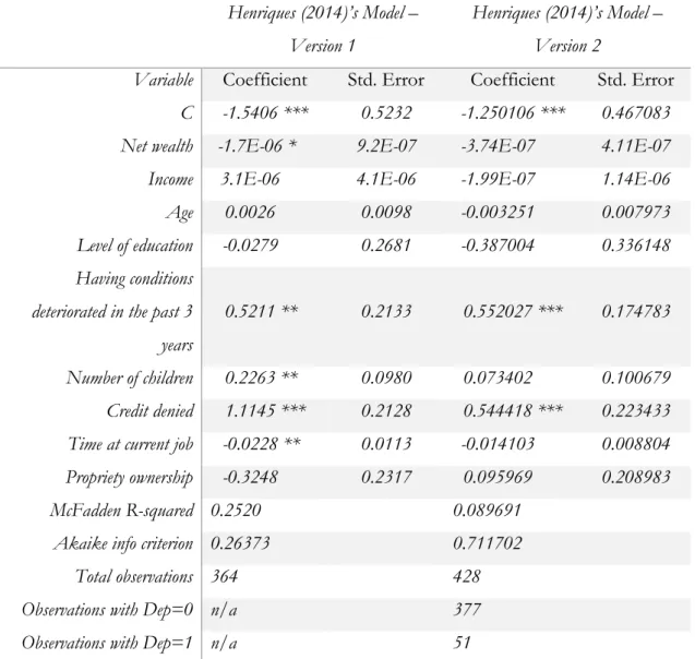
Table 11: Model developed by Catarina Henriques (2014)’ model – version 1 and 2 *: p-value < 0.1 **: p-value < 0.05 ***: p-value < 0.01 n/a: information not available. ... 46
Table 12: Accuracy rates of Model A, Model B, Henriques (2014)'s Model – Version 1 and Henriques (2014)'s Model – Version 2, with a cut-off equal to 15% ... 47
Table 13: Variables, values and weights of the rating model developed by Saunders and Cornett (2012) ... 49
Table 14: Accuracy of Saunders and Cornett (2012)'s model with the conversion of the variable “total gross income” from EUR to USD, with a range between 120 and 190 ... 49
Table 15: Accuracy of Saunders and Cornett (2012)'s model with the adjustment of the variable “total gross income” using PPP with a range between 120 and 190 ... 50
Table 16: Frequency of the scores from the model of Saunders and Cornett (2012) after the adjustment of the variable "total gross income" ... 51
xvi
Table 18: Accuracy of model C with a 15% accuracy rate, without discriminating the data of the countries ... 55
xvii
List of Annexes
Annex 1.: Market share calculation based on 2015 applicable turnover from credit rating activities and ancillary services in the EU (European Securities and Markets Authority, 2016).
... 65
Annex 2.: Initial 68 variables considered. ... 66
Annex 3.: Variables which outliers were controlled, and respective minimum and maximums (before and after the winsorization process) and respective percentage of winsorization. .. 68
Annex 4.: Variables tested and respective results (the ones in red are the ones that were automatically excluded due to their results in any one of the tests or for not being available). ... 70
Annex 5.: Distribution of the variable “situation at current job”. ... 76
Annex 6.: Distribution of the variable “Sector of the company where it has main job”. ... 77
Annex 7.: Distribution of the variable “Year of the acquisition of the main residence”. ... 78
Annex 8.: Accuracy of the models A and B, using cut-offs equal to 50%, 30%, 20% and 10%. ... 79
Annex 9.: Accuracy of Catarina Henriques (2014)’s model, using cut-offs equal to 50%, 30%, 20%, 15% and 10%. ... 82
Annex 10.: Accuracy of Catarina Henriques (2014)’s regressed model, using cut-offs equal to 50%, 30%, 20%, 15% and 10%. ... 84
Annex 11.: Accuracy rates of Saunders and Cornett (2012)’s model, using ranges between 240 and 310; 250 and 320; 260 and 330; 270 and 340; and 280 and 350. ... 86
Annex 12.: Accuracy rates of model C with aggregated data from Portugal, France, Italy and Spain, for cut-offs equal to 50%, 30%, 20% and 10%. ... 88
xviii
Annex 13.: Accuracy rates of model C discriminating the data from each country (Portugal, France, Italy and Spain), for cut-offs equal to 50%, 30%, 20% and 10%. ... 90 Annex 14.: Output of model C when regressing individually for each country; and respective accuracy rates, for Portugal and Spain, for cut-offs equal to 50%, 30%, 20%, 15% and 10%. ... 97
xix
List of Abbreviations and Acronyms
ANN Artificial Neural NetworksBCE Banco Central Europeu
BIS Bank for International Settlements DA Discriminant Analysis
DF Degrees of Freedom DT Decision Trees
ECB European Central Bank
HFCS Household Finance and Consumption Survey INE Instituto Nacional de Estatística
IRB Internal Ratings-based Approach
ISFF Inquérito à Situação Financeira das Famílias Logit Logistic Regression
LR Linear Regression
NAIC National Association of Insurance Commissions
OECD Organization for Economic Co-operation and Development PD Probability of Default
1
Chapter 1:
Introduction
Financial institutions, in their daily activities, perform the indispensable function of channeling funds from people that have surplus funds (suppliers of funds) to those with shortage of funds (users of funds), through credit. This process starts with the initial loan application and ends with the successful repayment of the loan or its default. Due to asymmetric information, the default is hard to predict because who borrows money has always more information than the one who lends (Kocenda & Vojtek, 2009). Uncertainty also makes complicated to forecast who will default and who will repay the loan. Although retail lending is one of the most profitable investments in a lender’s asset portfolio. The increase number of conceded loans also increases the number of defaulted ones. This arises a risk commonly known as credit risk. It exists since the existence of lending itself, back as far as 1800 B.C.E1. and the concept has been the same since the ancient Egyptian times
(Caouette, Altman, & Narayanan, 1998). Credit risk is the risk that a borrower may not repay a loan, because it is not able or unwilling to, which means that the lender may lose the principal and/or the interest associated with it. This risk arises because it is not possible to ensure that the borrowers will pay back the amount borrowed. According to Obrova (2012), credit risk can also be called “loan risk” and Caouette et al. (1998, p. XV) defines credit as being “nothing but the expectation of a sum of money within some limited time” and, consequently, defines credit risk as “the chance that this expectation will not be met”. There is credit risk anytime someone takes a service or a product, without paying immediately for it.
Over the last decades, credit risk measurement had to evolve radically, due to a number of reasons. According to Altman and Saunders (1997); Caouette et al. (1998); Hand and Henley (1997) some of the reasons include: (i) a worldwide increase in the number of
2
bankruptcies, translating into a more concern regarding credit risk; (ii) a trend towards disintermediation by the highest quality and largest borrowers, by investing directly in the money markets; (iii) the increase of competition; (iv) a declining value on real assets, translating in a decrease value of collaterals; (v) the drive for diversification and liquidity; (vi) an increase growth of off-balance sheet instruments with inherent default risk exposure; and (vii) regulatory changes, such as the requirements created by the Basel Committee on Banking Supervision2. Happily, in the last two decades, it had become easier to develop risk
measurement approaches due to the development of technology and the availability of information through the World Wide Web. Banks need to make use of this increasing sophistication in terms of techniques, strategies and scientific and mathematical models to measure the credit risk of loans in order to price them correctly; and to set appropriate limits on the amount of credit extended to a client. As Caouette et al. (1998) state, managing risk is the same as creating a custom-made suit: it is crucial to measure the costumer’s needs and capacities to make sure the financing is a good fit. This is very important because the default of a singular borrower can have a significant impact on the value and reputation of the financial institution. According to Constangioara (2011, p. 162), there is an urgent need to develop methodologies to assess credit risk since the development of the markets has led to “over-indebtedness and consumer bankruptcy phenomena”, especially after the financial crisis of the last decade. Thanks to this, academics and practitioners have started developing new and more sophisticated credit scoring systems and models to protect both the lenders and the good borrowers (which potentially will access to better conditions as lower is the rate of default of the other clients).
Having this in mind, and considering the fact that I was an intern at Banco L. J. Carregosa, the idea of this study is to develop a credit-scoring model to assess the creditworthiness of private clients of the Portuguese banking industry, considering their default probability, having in mind a work previously done by Henriques (2014) and to overcome her results. It is important to develop such model, because, in the United States (U.S.), it is used the FICO Score in 90% of lending decisions (Sousa, Gama, & Brandão,
2 The Basel Committee on Banking Supervision is a committee of banking supervisory authorities, which goal
is to provide a forum for regular cooperation on banking supervisory matters, to enhance understanding of key supervisory issues and to improve the quality of banking supervision worldwide. It was established in 1974.
3
2016) but, in the OECD3 countries (where Portugal and many European countries are
included), banks follow the approach proposed by the Basel Committee in which each bank is encouraged to develop its own internal scoring model (Bank for International Settlements, 2006). In order to do so, it is important to collect a data set, which will be the responses to a survey made by the European Central Bank (ECB) - the European Household Finance and Consumption Survey (HFCS)– in conjunction with several countries on the European Union, including Portugal. This survey provides sociodemographic and finance information about households that is indispensable to the creation of a good retail credit-scoring model. The lack of retail models in the industry is mainly due to the scarce information about households (because they are informationally opaque and borrow relatively infrequently (Kocenda & Vojtek, 2009)); the costs associated with retrieving such information; and the difficulties that banks face when trying to access the existent databases. Hence, with the development of the credit model for retail banking, we think this study will be useful to the banking industry of the European countries since it may be used by any financial institution that feels it is appropriate to its business.
The rest of the study proceeds as follows: chapter 2 presents the literature review; chapter 3 provides a comprehensive description of the data and the methodology followed; chapter 4 presents the model developed, its analysis, and a comparison with other models in the literature; chapter 5 presents an implementation of the model developed on other countries, namely France, Italy and Spain; and, at last, chapter 6 presents the conclusions and suggestions for future research.
3 OECD translates to Organization for Economic Co-operation and Development, which is an
intergovernmental economic organization with 35 country members, founded in 1960, in order to stimulate economic progress.
5
Chapter 2:
Literature Review
Part A.
1.1 Corporations vs. Retail Loans
The focus of this study, as previously mentioned, it to identify, develop and compute a credit model for private clients of the banking industry. Since “financial institutions manage credit risks
for business and consumers differently” (Šušteršič, Mramor, & Zupan, 2009, p. 4736), it is relevant to make a small distinction between lending to corporations and lending to individual borrowers. The Bank for International Settlements (2001, p. 55) (BIS)4 defines retail credit
as “homogeneous portfolios comprising a large number of small, low value loans with either a consumer or business focus and where the incremental risk of any single exposure is small”. These types of loans include loans made to individuals, such as credit cards, residential mortgages and home equity, auto or educational loans (Allen, DeLong, & Saunders, 2004). The differences between corporate and retail loans rely on the amount lent to each one of them, being much smaller to retail; and, while for corporate loans various financial ratios are used to construct models to assess credit risk or the probability of default (PD), like the z-score developed by Altman; in retail banking, various sociodemographic characteristics are collected to make a proper decision about the client. Moreover, since lenders face fixed costs when lending, lending to individuals become more expensive per dollar lent. Another disadvantage of lending to small firms or individuals is the lack of information since they tend to be more informationally opaque. Their information is not public.
4 The BIS is an international financial organization owned by 60 member central banks, headquartered in Basel,
Switzerland. It was established on 17 May 1930, and its mission is to serve central banks in their pursuit of monetary and financial stability.
6
Despite these disadvantages, it is still important to pay attention to credit conceded to individuals. According to statistics of Banco de Portugal, discounting the numbers to December 2016, the credit stock conceded to individuals in Portugal amounted €125 billion, of a total of €203 billion. As it can be seen, €125 billion is a huge number and, in percentage, refers to 61.58% of the total credit conceded by the financial sector (Banco de Portugal, 2017). Moreover, in the first nine months of 2017, the amount of credit conceded to consumer credit amounted to €17.7 million per day, a 12% increase in homolog terms. This increases the concern that Banco de Portugal has in relation to credit risk since it fears that households are falling into a “spiral of indebtedness”, again (Soares, 2017).
1.2 Traditional Approaches to Credit Risk
As Allen et al. (2004); Altman and Saunders (1997); Hand and Henley (1997) among others, state, in the last 30 years, some methodologies to assess credit risk among financial institutions were developed. The traditional ones focus on estimating the PD’s, including the probability of a bankruptcy filing, default or liquidation. According to the BIS, a client is in default if it is more than 90 days overdue with a payment connected with the loan; and, according to Banco L. J. Carregosa (2017), the default takes place when a payment is not made at the predetermined date.
Some examples of these traditional models include expert systems (where artificial neural networks can be included); rating systems; and credit scoring models.
1.2.1 Expert Systems
Expert systems rely on the subjective capacity of professionals in assessing the likelihood of default, according to some personal characteristics. Individuals become experts over the course of their careers, gaining authority as they acquire experience and demonstrate skills (Caouette et al., 1998).
One prominent example of such systems is the 5 C’s of credit: character, capital, capacity, collateral, and cycle. The first one, character, is related to the reputation of the potential borrower. It is a measure of the borrowers’ willingness to repay and his/her repay history. The second one, capital, is the leverage of the borrower. Capacity concerns the ability to repay, which reflects the volatility of the borrower’s earnings. Regarding collateral, it means that a banker has claims collaterals pledged by the borrower. The collateral depends on the PD that the professional believes the borrower has. Finally, the cycle conditions refer to the state of the business cycle. This last “C” is very important because a client, that seems
7
to be very independent of the state of the economy, may be affected by economic downturns and financial crisis (Allen et al., 2004; Altman & Saunders, 1997; Gonçalves, Gouvêa, & Mantovani, 2013).
In order to develop a more objective expert system, the artificial neural networks (ANN) have been introduced. Basically, an ANN uses historical repayment experience and default data to assess the PD of a client. Each time the network evaluates the credit risk of a new loan opportunity, it updates the data in order to “continually learns from experience” (Allen et al., 2004, p. 734). This feature makes the ANN a system very flexible and adaptable (Abdou & Pointon, 2011; Altman & Saunders, 1997) and it works due to the development of technology and the appearance of new methodologies, like artificial intelligence.
Since the network fits a system of weights to each financial variable included in the database, the downturn of the methodology lies on the fact that “too much training” may result in poor out-of-sample estimates. This can happen because the network may be “over fit” to a particular database (Allen et al., 2004), losing its universal characteristic. Allen et al. (2004) also underline the fact that it is very costly to implement and maintain this methodology, it is a slow procedure, and it may miss transparency through the process.
1.2.2 Rating Systems
A rating system was born to answer the question “How do lenders determine the creditworthiness of potential borrowers and assure themselves of the continued soundness of borrowers after a loan has been extended?” (White, 2002, p. 44). In order to answer the question, financial intermediaries may develop the necessary information themselves to construct a rating system or may turn to credit rating specialists, known as Credit Rating Agencies. These agencies can help those who cannot create rating systems themselves, by eliminating asymmetric information that surrounds the lending relationships.
A firm’s credit rating is a measure of the firm’s propensity to default. Credit ratings provide individual and institutional investors with information that assists them in determining whether issuers of debt obligations and fixed-income securities will be able to meet their obligations with respect to those securities.
Internal credit ratings are a progressively more important element of credit risk management. Within the past few years, the credit-related businesses have become gradually more complex and the number of counterparties has grown rapidly. Thanks to this, many banks, especially the bigger ones, have introduced more structured and formal systems for approving loans, portfolio monitoring, and management reporting. Internal ratings are
8
crucial inputs to all such systems as well as to quantitative portfolio credit risk models, like the one proposed by the Basel Committee.
Just like a public credit rating produced by credit rating agencies such as Fitch Ratings, Moody’s or Standard & Poor’s, a bank’s internal rating summarizes the risk of loss due to failure by a given borrower (Treacy & Carey, 2000). The main difference between the ratings produced by agencies and banks rely on the fact that internal ratings are assigned by bank personnel and are usually not revealed to outsiders, due to competitive advantage issues.
The National Association of Insurance Commissioners (NAIC)5 requires companies
to rank their assets according to six different classifications corresponding to the following credit ratings: A and above, BBB, BB, B, below B and default. But, currently, the specifics of internal systems vary across banks. Each one assigns grades and its associated risk according to their needs and typical clients (Allen et al., 2004).
The drawback of this credit assessment methodology relies, mainly, on its complexity. In order to develop an internal rating system, considerations about costs, efficiency of information gathering, consistency of ratings produces, and staff incentives must be made (Treacy & Carey, 2000).
1.2.2.1 Rating Agencies
Credit rating agencies (such as Moody’s Investors Service; Standard & Poor’s Corporation; or Fitch Ratings) provide investors a forward-looking opinion on the relative credit risks of financial obligations, such as interest, preferred dividends, repayment of principal, insurance claims or counterparty obligations (Fitch Ratings, 2017; Moody's Investors Service, 2017). It is their job to inform investors about the likelihood of them receiving their money back, as scheduled for a given security. Despite what many may think, it is not their job to make recommendations about buying or selling; their job is only to express informed decisions about creditworthiness, through independent, objective, transparent and high-quality analytic processes (Caouette et al., 1998). This does not mean, however, that, in the theoretical approach, credit ratings should be exclusively attributed by a commercial rating agency. In fact, many major financial institutions maintain their own credit rating systems, based on internally developed methodologies (internal ratings), as it was already mentioned. Moreover, just because these agencies are specialized in attributing
5 The NAIC is the U.S. standard-setting and regulatory support organization. It establishes standards and best
9
ratings, that does not mean that they are accurate. The rating is just an opinion. As Fitch Ratings (2017, p. 4) states, “ratings are not facts and, therefore, cannot be described as being «accurate» or «inaccurate»” and “users should refer to the definition of each individual rating for guidance on the dimensions of risk covered by such rating”.
Despite that, rating agencies are especially important for borrowers, since they facilitate their access to new markets and diminish the costs of their borrowings. Individuals with no expertise in financial markets can easily enter the market by buying the services from these agencies.
Nowadays, the three biggest players are Fitch Ratings, Moody’s Investors Services and Standard &Poor’s (S&P). These three rating agencies provide extensive rating coverage in Europe, especially Moody’s and S&P. Despite the existence of more than 30 other rating agencies in Europe, these three dominate the market with a market share of more than 90% (see Annex 1).
Each one of these agencies uses a system of alphanumeric letter grades to allocate the issue or issuer on a spectrum of credit quality. The spectrum goes from AAA/Aaa (very low probability of defaulting or a strong capacity to meet financial commitments) to C/D (very high probability of defaulting). The higher the grade, the higher is the probability that principal and interest payments will be paid. The debt rated Baa3/BBB- or above is considered to be of investment grade quality; while issues rated below Baa3/BBB- are viewed as speculative and risky.
Recently, on September 2017, Portuguese Republic’s credit rating was restored to investment grade by S&P, going from BB+ to BBB-; and by Fitch Ratings, going from BB+ to BBB+, on December 2017. It was BB+ since 2012 when the country was going through a bailout program provided by the European Union and the International Monetary Fund (Lima, 2017). This means a lot to Portugal. As the current Portuguese Finance Minister, Mario Centeno, states:
[The upgrade of the country’s credit rating] “(…) allows a much vaster array of investors to have Portuguese debt in their portfolios. It also allows private debt to benefit from these better financing conditions, and this is very relevant for Portuguese banks” (Lima, 2017).
1.2.3 Credit Scoring Models
A credit scoring model is “the term used to describe formal statistical methods used for classifying applicants for credit into good and bad risk classes”, as states Hand and Henley (1997, p. 523) and it is considered as “one of the most successful applications of statistics and operations research” (Crook,
10
Edelman, & Thomas, 2007, p. 1448). According to Thomas (2000, p. 151), “credit scoring is essentially a way of recognizing the different groups in a population when one cannot see the characteristic that separates the group but only related ones”. According to the same author, this idea was first introduced by Fisher, in 1936, and then developed by Durand, in 1941, who was able to recognize that the separation of classes was useful to separate among good and bad loans.
Although credit risk is more than 5,000 years old, credit scoring models have just a little more than 50 years (Samreen and Zaidi, 2012). The first one appeared in the 1950’s when the first consultancy of credit risk was formed by Bill Fair and Earl Isaac (Baker & Filbeck, 2013). In the late 1960’s, with the development of credit cards and with the need for more automatic decision-making processes, banks and some credit cards issuers realized the importance of credit scoring models (Thomas, 2000). Only some years after, the use of credit scoring techniques was extended to other products, like home loans and small business loans (Thomas, 2000). In the 1980s, with the development of technology science, new methodologies were developed to compute more advanced scorecards, like logistic regression and linear programming. More recently, artificial intelligence techniques, like neural networks, appeared (Thomas, 2000). The first banks to use scoring models for small businesses were mainly big banks that had at their service historical loan data to build a robust model, like Hibernia Corporation, Wells Fargo, BankAmerica, Citicorp, NationsBank, Fleet and Bank One (Mester, 1997).
Statistical models, also called score-cards, were developed through the years and they “use predictor variables from application forms and other sources to yield estimates of the probabilities of defaulting” (Hand & Henley, 1997, p. 524). The decision to whether grant or not credit is made comparing the PD with a predefined threshold. Nowadays, standard statistical models include discriminant analysis (DA), linear regression (LR), logistic regression (logit), probabilistic regression (probit) and decision trees (DT) (Constangioara, 2011; Costa & Farinha, 2012; Hand & Henley, 1997). The two most used ones are the logit and the DA, which was pioneered by Altman in 1968 (Allen et al., 2004). The downturn of the DA relies on the fact that assumes linearity between variables, which is not always true. On the other hand, the logit is better because do not require the multivariate normality assumption (Šušteršič et al., 2009).
11
Method Main technique Summary
Linear regression Ordinary Least
Squares
Determine formula to estimate continuous response variable.
Discriminant Analysis Mahalanobis distance Classify cases into prespecified groups, by
minimizing in-group differences.
Logistic Regression or Probabilistic Regression
Maximum likelihood estimation (MLE)
Determine formula to estimate binary response variable.
Decision trees RPA’s Uses tree structure to maximize group
differences. Complex for large trees.
ANNs Multilayer perception AI technique, whose results are difficult to
interpret and explain.
Linear programming Simplex method Operation research technique usually used for
resource allocation optimization. Table 1: Different methods to construct a credit scoring model and respective technique and summary
Source: Anderson (2007)
All these different models use financial variables that are believed to have statistical explanatory power in differentiating defaulting firms from non-defaulting and sociodemographic variables to assess the possibility of having individual clients defaulting. The variables can be related to the client’s stability, like time at current address and/or job; regard financial sophistication, like the possession of checking accounts, savings accounts, credit cards and time at the current bank; or related to the consumer’s resources, like his/her ownership status, employment and number of children (Obrova, 2012, p. 661). However, characteristics such as race, religion, national origin, gender, color or marital status cannot be used in the U.S.6 and should not be used due to racism and prejudice. After the parameters
of the model are assessed, the loan applicants are assigned a score that classifies the loan as good or bad, that can be, consequently, converted into a PD.
According to Mester (1997), 97% of banks use credit scoring for approve credit cards applicants; and 70% use it to their small business lending.
The credit scoring has the advantage that a loan can be conceded independently of its location since the process can be done without a face-to-face contact. Documentation is minimal; it is inexpensive to implement, without subjection like the expert models (Allen et al., 2004). But, on the other hand, data limitations, the so called “population drift”, sample bias
12
and the assumption of linearity are the downturns of this methodology (Allen et al., 2004; Altman & Saunders, 1997; Hand & Henley, 1997).
Despite what happens among European countries, in the U.K. and in the U.S. people are being credit scored or, as Thomas (2000) states, “behavior scored”, at least once a week. This is mainly done through the “FICO model” and it aims to monitor the clients’ propensity to default.
1.2.3.1 FICO Model
The most used credit scoring model today is the one developed by Fair, Isaac and Co. Inc. – the FICO model. This model was specially developed to meet the needs of individual costumers, who needed credit. Over the years, the model was developed to cover other business areas, such as to evaluate credit of small businesses, including trade credit (CrediFYI.com) or loan credit (LoanWise.com). In 2001, the original FICO model was improved and costumers could determine their credit score using the internet, through the website myfico.com.
As there is the FICO score, there are other credit scores across banks and firms. Usually, the differences between them are the variables that compose the model. For example, the FICO score uses variables related to credit history and credit reports to determine a score that goes from 300 to 850. The authors of this score choose to not include variables that are capable of bias a lender, such as race, religion, national origin and marital status (Allen et al., 2004).
The FICO score and scores alike exist mainly in the U.S.A. and in the U.K.. It is not a methodology usually followed by European banks. This happens due to three different reasons. First, there is lack of information about households, since they are informationally opaque and do not have their own information public, which complicates the creation of a robust model. Second, despite the existence of some surveys made to households about their financial stability, banks face many difficulties when trying to access them. At last, even if banks had all the information that was needed to create such models, there are costs associated with the creation of a credit scoring model. Since individuals borrow less money when comparing to big clients and corporations, it becomes more expensive, per dollar/euro lent, to create a good credit scoring model to individual clients (Kocenda & Vojtek, 2009).
13
1.3 BIS Basel New Capital Accord
The Basel Committee on Banking Supervision is an important player when concerning the financial risk regulation network, by setting risk management regulations to financial institutions all over the world. It was established in 1975 by the Central Bank Governors of the Group of Ten (G10) countries, with representatives of 13 different countries (Belgium, Canada, France, Germany, Italy, Japan, Luxemburg, the Netherlands, Spain, Sweden, Switzerland, the United Kingdom and the United States); and meets regularly in Basel, at the Bank for International Settlements.
The (first) Capital Accord (Basel I) was released in July 1988, in order to establish a minimum capital standard to protect financial institutions against credit risk. In 1993, the market risk was included in the scope of the accord. In 1998, the accord was fully reviewed in order to take into account all risks faced by financial institutions, including the operational risk, and, thanks to that, a new Basel accord was created – the Basel II.
The proposed Basel New Capital Accord allows banks to choose which approach they prefer when determining their capital requirements – capital that is set aside to cover unexpected losses. Regarding credit risk, there are two approaches that banks can follow: the Standardized Approach, which is a standardized manner to assess credit risk, supported by external credit assessments (like Rating Agencies); and the Internal Ratings-based Approach (IRB), that allows banks to use their own internal rating system (subject to prior approval by the National Supervisor) (Bank for International Settlements, 2006).
White (2002) criticizes the proposal by the BIS, by saying that it only creates demand to rating agencies and do not designate how credit rating firms should be certified. This happens because, in order to the Standardized Approach to be effective, banks can only rely on credit ratings by firms that are certified – ECAI’s (External Credit Assessment Institutions). Moreover, as White (2002, p. 56) states, “adoption of the BIS proposal in its current form is thus likely to raise worldwide barriers to entry into the credit rating industry”, since it is only advantageous, for the rating firms, if they can be certified, otherwise they would lose a relative amount of possible clients. In relation to the IRB approach, Crook et al. (2007) believe that big banks tend to choose this approach because it allows banks to have less capital, earning higher returns on equity, since they are more or less free to choose the model to be used.
14
Part B.
In order to develop a credit-scoring model or any model, some steps must the chronological followed. First, it is important to collect information about the population. Some surveys are available to research, like the one that will be the base of this study - the Household Finance and Consumption Survey (2013), inquired by the European Central Bank (ECB). Secondly, it is fundamental to investigate which type of model will produce the best results to the objective in question: LR, DA, logit, probit, ANNs, among others; and which set of variables to include in the model. Then, the model must be run and some tests to infer its significance and adequacy to the purpose in question must be made. Only after going through these steps, it is possible to assess if the model developed was made properly and is adequate to the final objective that it is to assess the creditworthiness of retail clients of the European banking industry.
West (2000) believes that ANNs perform better when assessing the creditworthiness of clients, but that the logist is a good alternative. In order to evidence that, the author conducted a study using two databases – German and Australian credit data – to assess which models and types of models are more suitable: parametric models (like DA and logit), nonparametric methods (like k nearest neighbor and kernel density), DT’s or ANNs. The author concluded that ANNs models can increase the credit scoring accuracy from 0.5 to 3%, which can save millions to the financial institution; that the best ANNs to assess the creditworthiness of clients are mixture-of-experts and radial basis function neural networks; and that the logit is indeed a good alternative, since the difference in terms of accuracy is very small when comparing to ANNs.
Šušteršič et al. (2009) created a credit scoring model using ANNs. Using a data set provided by a Slovenian bank with internal bank data available for 581 short term consumer loans in the period of 1994 to 1998, and comparing with a logit model, the authors came to the conclusion that EBP ANNs (the type of ANNs used) have the best accuracy and the lowest value for error type II, with 79.3% of accuracy, 17.8% error type II and 29.9% error type I. The main objective of this study was to conclude about the variable selection method used, which was a principal component analysis and a genetic algorithm (Kohonen neural network and random method). The model started initially with 67 variables and ended with only 21. The author chose to make a comparison between ANNs and LR because “the logit model is the most promising and widely used statistical credit scoring model” (Šušteršič et al., 2009, p. 4750).
15
On the same line of research, Imtiaz and Brimicombe (2017) conducted a study to verify which model is the best to assess the creditworthiness of clients when imputation technique7 is used and when it is not. The authors concluded that ANNs present better
results when the imputation technique is applied, since it increases the availability of data and, therefore, increases the accuracy rate of classification of ANNs. In the absence of the technique, the author concluded that, despite having DT’s performing better when training the model, ANNs performed better when the model was tested. Despite the overall better accuracy of ANNs models, its downturns rely on the fact that it takes too much time to train the model when there is a big sample, which is when the model presents its better results. Moreover, according to the author, and in the context of risk control, it is more meaningful to test the client risks without imputation, since it can bias the sample.
Samreen and Zaidi (2012) conducted a study to assess which type of model produced the better results when assessing the creditworthiness of Pakistan’s clients. The author interviewed 250 clients of the banking industry of Pakistan and concluded that the logit regression had an accuracy rate of 98.8% and the DA for individuals presented an accuracy rate equal to 95.2%. The variables used by Samreen and Zaidi (2012) included sociodemographic variables, such as marital status, age, number of dependents, occupation, working period with the last and current employer, and monthly net income; and finance related variables, such as loan tenure, loan period, banking references at the bank, credit history and loans from others banks.
Table 2 summarizes the different conclusions, in terms of total accuracy, that the different authors determined, as well as the technique used to assess the accuracy – AUC or Error Rate.
Author (year) Logit ANNs DA CT’s Database Obs.:
(West, 2000)
76.30% 77.57% 72.60% 69.56% From
German
Accuracy technique used: Error Rate
87.25% 87.61% 85.96% 84.38% From
Australia
Accuracy technique used: Error Rate (Šušteršič et al., 2009) 76.10% 71.30% 79.3% 73.00% - - From Slovenia Selection variable technique
7 Imputation technique is a technique that it is used when there are missing values in the sample, by replacing
missing values with substitute data. It presents some advantages like avoids the decrease in the number of values of the sample that it is studied; but may introduce bias and reduce efficiency.
16
72.00% 70.70% Accuracy technique used:
Error Rate (Samreen &
Zaidi, 2012) 98.80% - 95.20% -
From Pakistan
Accuracy technique used: Error Rate (Constangioara, 2011) 96.00% 74.80% 96.00% 74.80% - 96.00% 74.20% From Hungary Stepwise selection Accuracy technique used:
Error Rate and AUC (Kocenda & Vojtek, 2009) 86.40% 83.20% - - 83.00% 80.40% From The Czech Republic
With and without “Own resources” Accuracy technique used:
AUC (Imtiaz and Brimicombe, 2017) 90.29% 86.18% 90.99% 87.90% - 89.57% 79.09% From Taiwan Without imputation technique Accuracy technique used:
Error Rate and AUC
Table 2: Overall accuracy of the models developed by the authors
As it can be seen from the previous table, ANNs models seem to be the most accurate ones but just with a minimal difference from logit regressions. Despite the fact that DA is one of the most used ones, its accuracy is not that great when comparing to other models. The main reason why DA is still one of the most used models today relies on the fact that institutions developed DA models in the past and are now reluctant to develop better models, due to the costs associated with it and the time it consumes. According to Hand and Henley (1997, p. 535), there is no best model. It depends on “the data structure, the characteristics used, the extent to which it is possible to separate the classes using those characteristics and the objective of the classification”. And a model to considered as “best”, does not depend only on the accuracy of the classifications as “good” or “bad”, but also on the speed of the classification, the speed on which it can be revised and on the clarity of the model. According to these authors, ANNs are not good models due to their complexity and characteristic of “black boxes”; therefore, a model that is more intuitive and appealing is preferable, to clients and users, such as logistic regressions, probabilistic regressions and tree-based methods.
Alfaro and Gallardo (2012) conducted a study to assess what are the main determinants of consumer and mortgage default, at the household level in Chile, using data from the Survey of Household Finances made in 2007. The authors concluded that, at the consumer level, the main determinants are income-related variables, such as the number of people in the household that contribute with income; as well as the debt service ratio. At the
17
mortgage level, the authors also concluded that income-related variables are important, such as having a bank account and an education level beyond high school.
Besides the importance of sociodemographic and finance related variables (Abdou & Pointon, 2011; Avery, Calem, & Canner, 2004; Caouette et al., 1998; Constangioara, 2011; Costa, 2012; Gonçalves et al., 2013; Hand & Henley, 1997; Obrova, 2012) in order to construct a reliable model, it is also important to add variables that translate the change of the economic, health, or other conditions that may affect the ability of the client to pay back the money that was borrowed (Avery et al., 2004; Costa, 2012). This may be a health disease of some member of the family/household; a natural catastrophe, like the fires in Pedrogão Grande (Portugal), on June 2017; or some other unexpected “economic or personal shock” (Avery et al., 2004, p. 854). This is important because there are some circumstances that the client do not control and, therefore, are not related to its personal characteristics.
Just for curiosity, in 1982 some of the variables included in credit scoring models were if the household had a telephone at home and/or at the office, or not; the age difference between husband and wife; the zip code; and personal characteristics that nowadays are not allowed, like race, religion, sex, marital status and ethnic origin (Capon, 1982). This is relevant because highlights the importance of adapting the model as the years go by. With the development of technology, society, economy and with the emergence of new discoveries, the models must the adapted to translate the truth about individuals and their mutable behavior.
Table 3 presents the most used variables in the studies conducted by some authors. As it is possible to assess, variables related to sociodemographic information are the ones that appear the most, like income-related variables, age, marital status and level of education. On the other hand, despite the fact that they do not appear as much as sociodemographic information, variables related to the household’s finances/credit history are also important, like having, or not, a bank account and a credit card, and having credit denied in the past.
18 Ne t we alth Deb t Inco m e Age Educa tion T im e at cu rr ent j ob Pe rs ona l shoc ks Num ber o f d epen de nts Havin g c re dit d enied Ho m e pro priety R eg ul ar e xp ense s Jo b situa tion M ortg age s Gend er M arita l sta tus Ba nk a cco un t T im e at cu rr ent a dd ress Ho m e pos tco de T ype o f cre dit O ccup ation T im e at l ast jo b L oa n ten ure L oa n p er io d C re dit h isto ry Greene (1992) x x x x x x x x x x x
Hand and Henley (1997) x x x x x x x x x x
Constangioara (2011) x x x x x x x
Alfaro and Gallardo
(2012) x x x x x x x
Costa (2012) x x x x x x x x x
Samreen and Zaidi (2012) x x x x x x x x x x
Gonçalves et al. (2013) x x x x x x x x x Henriques (2014) x x x x x x x x x x Absolute frequency 1 3 8 8 4 5 2 5 1 3 2 2 1 2 5 3 3 2 3 5 1 1 1 2 Relative frequency 12.5% 37.5% 100% 100% 50% 62.5% 25% 62.5% 12.5% 37.5% 25% 25% 12.5% 25% 62.5% 37.5% 37. 5% 25% 7.5% 62.5% 12.5% 12.5% 12.5% 25%
19
Chapter 3:
Data Description & Methodology
This chapter intends to describe the data used to develop this study as well as the methodology followed to pursue it, including basic statistical techniques and more advanced hypothesis tests. The chapter concludes with the description of the 27 variables that passed the different tests conducted and are, therefore, suitable for the development of the model that this study is trying to develop.
Part A: The Survey
The data used to develop this study was retrieved from a survey conducted by the European Central Bank in conjunction with the central banks of the Euro system and three National Statistical Institutes, in 2013. The survey, entitled “Household Financial and Consumption Survey” – HFCS -, provides detailed information on various aspects of European households, namely sociodemographic and financial information. The main questions of the survey are related to the property of the households inquired, like financial and fixed assets possessed; to possible loans that use those assets as collateral; as well as other financial obligations and applications. The survey includes, also, questions regarding heritages, income and the households’ decisions about consumption and savings, and questions regarding the individuals that compose the household, like age, level of education, and situation at the job.
The survey is a decentralized one. Each country that have contributed to the development of the survey worked individually and independently on their country. The Portuguese contribution was conducted by Banco de Portugal in conjunction with the Portuguese National Statistic Institute, which was one of the three National Statistics Institutes involved. The survey made by Portuguese entities is entitled “Inquérito à Situação Financeira das Famílias” – ISFF -, and it was conducted two times, one in 2010 and the other in 2013. The ISFF is composed by the same questions of the HFCS (designated as core
20
variables) as well as some questions oriented to the Portuguese type of families only. The 2013 survey inquired 8,000 Portuguese families that have resulted in 6,207 final households.
The Portuguese contribution is composed by more than 700 different variables, in which part of them concerns the household as a whole and the some concern each individual that composes each household, resulting in more than 16,000,000 observations, separated in 5 different files.
Part B: Methodology
As it was mentioned in the last chapter, in the past, credit institutions and credit analysts used their knowledge and prior experience when assessing the probability of default of some client. Later, that technique was systematized into the 5 C’s of credit.
The authors in the literature defined 5 C’s of credit: character, capital, capacity, collateral and cycle conditions. This study will consider the 5 C’s of credit to assign an initial economic intuition behind the variables to include in the model, since it helps and have helped professionals assessing the likelihood of default of some clients. This study will assume the same number of C’s but will substitute the first one – character – by a wider one – personal and socio-professional characteristics -, which is composed by three main sub-categories: “Personal characteristics & Educational background”; “Professional & Financial situation” and “Family situation”. This first “C” is important because gives a sense of the household’s character and stability that is very important to predict if the household may default or not. Moreover, it gives a sense of the number of people in the household and if they are contributing to the household main income. The second “C”, capital, is important because gives an idea of possible resources available to use if an undesirable situation happens, considering more liquid assets, like financial assets, that are not used on a daily basis for regular expenses. Capacity concerns the volatility of earnings and the ability of the household to repay its debts, like, for example, the variable “income”. Collateral is also an important category because gives the notion if the household have assets that may be set as collateral. At last, the cycle conditions are important because they influence everyone and may have a very negative impact, even if a household is very wealthy.
This division helps the choice of the variables to include in the model, since this study relies on the ISFF, which has more than 700 different variables. Of those 700 variables, 68 were first selected, having in mind the ones used by the authors mentioned (see Table 3) as well as some that appeared to be relevant, due to an economic intuition. All of them are presented in Annex 2, grouped by category.
21
These 68 variables were first divided in two groups – continuous and categorical variables – since the analysis is different for each category of variables; and then each group was also divided in two different groups: households that have defaulted in the past and households that have not. This separation is important to assess if there is any significant difference among households who have defaulted and who have not, by looking at their variances, means, proportions, etc. The objective of this separation is to see which variables have informative content that enables the differentiation of households who have defaulted in the past and households who have not.
The first thing to do was to see if the distributions of the continuous variables had outliers and, if so, the second step was to control them using a technique called winsorization. This step is important because it will be necessary to calculate the mean and variance of the default and non-default groups to see if it is possible to differentiate among them. So, it is crucial to control for outliers because, in a distribution that is heavily skewed, the sample mean may not be the best estimate, since the difference between two sample means may offer a poor summary of how the populations differ and the magnitude of that difference (Everitt, 1992). To do that, the simple interquartile range statistic technique was used:
- First it is calculated the 1st (1Q) and 3rd quartile (3Q);
- Then it is calculated the interquartile range (IQR), which is equal to the difference between the 3rd and the 1st quartile;
- Finally, a sample has upper outliers if:
3𝑄 + 1.5 ∗ 𝐼𝑄𝑅 < 𝑆𝑎𝑚𝑝𝑙𝑒 𝑀𝑎𝑥𝑖𝑚𝑢𝑚
And bottom outliers if:
1𝑄 − 1.5 ∗ 𝐼𝑄𝑅 > 𝑆𝑎𝑚𝑝𝑙𝑒 𝑀𝑖𝑛𝑖𝑚𝑢𝑚;
and the winsorization of the distribution was done using the software E-views. Basically, to “winsorize” a distribution is to give less weight to values in the tails of the distribution and to pay more attention on those near the center, by substituting the highest x% of scores to the next smallest score and to change the x% smallest score to the next largest score (Everitt, 1992). To winsorize a distribution is, in a certain way, better than to “trim” a distribution - which is to simply delete the x% largest and smallest scores -, because using the winsorization technique no observations are lost.
Then, the variables that had outliers were winsorized at a 1% level and, if they still had outliers, they were winsorized at a 2% level, and so on. The variable with the higher
22
percentage of winsorization was “Total Financial Assets”, with a winsorization level of 12%, as Annex 3 shows.
After this, the first test computed was the Chi-square independence test, to both variables (continuous and categorical ones), to test if there is independence between an independent variable and the dependent one. The idea is to exclude variables that do not have a significant association with the dependent variable. It is important to note, though, that the relationship that this test tries to capture is not necessarily causal: one variable does not “cause” the other. The test is the following8:
Test 1. Chi-square test of Independence H0: Variable A and variable B are independent
H1: Variable A and variable B are not independent 𝑋2= ∑𝑂𝑟,𝑐−𝐸𝑟,𝑐
𝐸𝑟,𝑐 ~𝑋
2(df)
where 𝑂𝑟,𝑐 is the observed number of observations in row r and column c of the contingency table; 𝐸𝑟,𝑐 is the number of estimated observations in row r and column c of the contingency table; r is the number of levels for one categorical variable; and c is the number of levels for the other categorical variable. The number of degrees (DF) of freedom is equal to:
𝐷𝐹 = (𝑟 − 1) ∗ (𝑐 − 1)
and the expected frequencies are computed separately for each categorical variable at each level of the other categorical variable, using the following formula:
𝐸𝑟,𝑐=
𝑛𝑟∗ 𝑛𝑐 𝑛
where nr is the total number of sample observations at level r of variable A, nc is the total number of sample observations at level c of variable B, and n is the total sample size.
To compute this test, it was constructed a contingency table for each variable to help perform it and interpret the results9. The variables whose test concluded that are independent
from the dependent variable were automatically excluded10. The ones that have passed the
test are the following:
8 Every test was computed using a significance level equal to 5%.
9 In order to conduct this test among the continuous variables, they were divided into different classes in order
to make this test feasible.
10 Since the significance level is considered to be 5%, the variables that presented a p-value higher than 5%
23
Nº Variable Chi-square Degrees of freedom P-value
1 Age 8.66 3 3.41%
2 Level of education 63.58 1 0.00%
3 Marital Status 8.87 1 0.29%
4 Level of education of the father 10.96 2 0.42%
5 Level of education of the mother 10.19 2 0.61%
6 Time at current job 23.92 4 0.01%
7 Credit denied 13.08 1 0.03%
8 Having a bank account 40.16 1 0.00%
9 Having credit card 40.16 1 0.00%
10 Having savings 175.7 1 0.00
11 Situation at current job 76 3 0.00%
12 Type of contract at current job 11.85 1 0.00%
13 Having another job 4.86 1 2.74%
14 Number of dependents 20.60 3 0.01%
15 Number of people in the household 38.22 5 0.00%
16 Number of people in the household
with a job 54.85 3 0.00%
17 Type of residence 8.49 3 3.68%
18 Total residence surface 39.94 4 0.00%
19 Occupancy scheme 32.66 3 0.00%
20 Financial Assets 212.77 1 0.00%
21 Income 137.81 4 0.00%
22 Total expenses 57.54 4 0.00%
23 Expenses of the last 12 months in
relation to income 246.28 2 0.00%
24 Expenses of the last 12 months in
relation to the average 11.03 2 0.40%
25 Capacity to get financial support by
friends and family 8.61 1 0.33%
26 Fixed Assets 91.59 4 0.00%
24 28
Having conditions deteriorated in the
past 3 years 55.47 1 0.00%
29 Sector of the company where it has the
main job 16 8 3.68%
30 Having conditions deteriorated in
next 2 years 5.74 1 1.66%
31 Year of the acquisition of the main
residence 5.74 1 1.66%
Table 4: Variables that have survived Test 1
After that, the variances and means for the defaulted and non-defaulted groups were computed:
Test 2. Variance difference test
Since there are two tests to compute the test for the difference between two sample means, one assuming equal variances and one assuming the opposite, a test to infer the equality of the variances was necessary, which assumes the following hypothesis:
H0: σ12 = σ12
H1: σ12 ≠ σ12
𝐹 =𝑠12
𝑠02~𝐹(𝑛1− 1; 𝑛2 − 1),
where n1 and n2 are the number of observations of sample 1 and sample 2, respectively; and
it is assumed that the population is normally distributed.
If the variances are assumed to be statistically different, Test 3.1 was computed, otherwise Test 3.2 was computed:
Test 3.1 Mean difference test with different variances H0: µ1=µ2 H1: µ1≠µ2 𝑡 =(𝑋̅1− 𝑋̅2) − (µ1 − µ2) (𝑠𝑝 2 𝑛1+ 𝑠𝑝2 𝑛2) 1/2 ~𝑡(𝑛1+ 𝑛2− 2)
where 𝑠𝑝2is the weighted average of sample variances and it is calculated as follows:
𝑠𝑝2=
(𝑛1− 1)𝑠12+ (𝑛2− 1)𝑠22 𝑛1+ 𝑛2− 2
25
Test 3.2 Mean difference test with equal variances H0: µ1=µ2 H1: µ1≠µ2 𝑡 =(𝑋̅1− 𝑋̅2) − (µ1 − µ2) (𝑠1 2 𝑛1+ 𝑠22 𝑛2) 1/2 ~𝑡(𝑑𝑓) 𝑑𝑓 = (𝑠1 2 𝑛1+ 𝑠22 𝑛2) 2 (𝑠1 2 𝑛1) 𝑛1 2 + (𝑠2 2 𝑛2) 𝑛2 2
Having in mind the last variable selection made using the first test, the continuous variables that have survived both tests are the following:
Nº Variable Mean Mean |
Default Mean | Non-default P-value (Test 2) P-value (Test 3.1) P-value (Test 3.2)
1 Age 56 years 48 years 50 years 0.54% 1.31% **
2 Time at current job 7.97 years 8.34 years 10.90 years 1.50% 0.00% ** 3 Total residence surface 129m2 124m2 137m2 41.89% * 0.00% 4 Financial Assets €18,421 €8,101 €19,060 0.00% 0.00% ** 5 Income €110,623 €86,596 €136,675 0.00% 0.00% ** 6 Total expenses €1,256 €1,243 €1,507 0.00% 0.00% ** 7 Fixed Assets €224,531 169,214€ €257,000 0.00% 0.00% ** 8 Wealth €160,203 €96,854 €160,564 0.59% 0.00% **
Table 5: Variables that have survived Test 3.1 and Test 3.2 *: Test 3.2 was computed given the acceptance of the null hypothesis on Test 2. **: Test 3.1 was computed given the rejection of the null hypothesis on Test 2.
As it can be seen when analyzing Table 4 and 5, all the continuous variables present in Table 5 are present in Table 4, which means that the difference in means test did not exclude any additional variable.
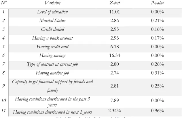
For the binomial categorical variables only, it was computed a binomial proportion test to assess if the difference in the proportions of observations “1” were statistically different, or not, from the ones equal to “0”. This test was made to exclude variables which