Abstract— The deployment of increasingly dense heterogeneous mobile networks can create high levels of interference among users which, combined with severe time dispersive channels, can result in substantial performance degradation. In order to cope with both effects, in this paper we propose an iterative block decision feedback equalizer (IBDFE) for single carrier (SC) transmissions which makes use of the correlation between the interference in the receiving antennas and minimizes the mean squared error (MSE) of the detected symbols. Our analytic and simulated performance results show that the proposed receiver can clearly outperform the conventional IBDFE and the linear interference rejection combining (IRC) detector in severely time-dispersive channels with strong cochannel interference.
Index Terms—Decision feedback equalizers, frequency-domain equalization, interference rejection combining, SC-FDE.
I. INTRODUCTION
The increasing demand for higher data rates in wireless services requires a continuous improvement of broadband wireless communication systems in order to deal with the limited spectrum resources, dispersion of the channel and interference between users. In order to tackle the intersymbol interference (ISI) caused by the channel time dispersion, most of the emergent wireless systems employ either orthogonal frequency division multiplexing (OFDM) [1] or SC [2] transmission techniques. While OFDM allows simple receiver implementations, it suffers from a large peak to average power ratio (PAPR) which leads to amplification difficulties, making it more suitable for the downlink. For the uplink, the use of single carrier block transmissions with frequency domain
Copyright (c) 2013 IEEE. Personal use of this material is permitted. However, permission to use this material for any other purposes must be obtained from the IEEE by sending a request to [email protected].
N. Souto, A. Correia and C. Reis are with the ISCTE-University Institute of Lisbon and Instituto de Telecomunicações, 1649-026 Lisboa, Portugal (e-mail: [email protected], [email protected], [email protected]).
R. Dinis is with the Instituto de Telecomunicações and Faculty of Science and Technology-UNL, Monte da Caparica Lisboa, Portugal, 2829-516 Caparica, Portugal (e-mail: [email protected]).
This work was partially supported by the FCT - Fundação para a Ciência e Tecnologia (projects ADIN - Advanced PHY/MAC Design for Infrastructure-less Networks PTDC/EEI-TEL/2990/2012, LTE-Advanced Enhancements using Femtocells PTDC/EEA-TEL/120666/2010 and PEst-OE/EEI/LA0008/2013).
equalization (SC-FDE) is often preferred due to its lower PAPR, while still being robust in ISI inducing channels [3]. This hybrid approach with OFDM for the downlink and SC for the uplink has been adopted by several wireless standards like the 3GPP Long Term Evolution (LTE) [4]. Although it is possible to employ low complexity linear receivers in SC schemes the performance is far from the matched filter bound (MFB) [5]. In order to improve the performance, nonlinear schemes like decision feedback equalizers (DFE) can be used instead [6] with one of the most promising being the IBDFE [7]-[9] based on the minimum mean squared error (MMSE) criterion. It employs feedforward and feedback filters implemented in the frequency domain and has been shown to be capable of performing close to the MFB in rich multipath propagation channels, especially when combined with diversity techniques [5][10].
In addition to the problem of channel dispersion, the deployment of denser heterogeneous systems where cells utilize the maximum available bandwidth can result in large levels of interference among users. This interference can be suppressed using several techniques like coordinated scheduling, cooperative processing or interference cancellation. Although techniques employed in spatial multiplexed receivers [11]-[14] can be used for removing interference, in addition to the main user they also require estimating the interferers’ streams thus adding substantial complexity. Therefore, among several interference cancellation techniques, the linear IRC [15] which avoids explicit knowledge of the interferers’ streams, is one of the most attractive due its simplicity and direct extension to the conventional MMSE detector and has been studied for use in 3GPP LTE systems [16]-[19]. While linear IRC detectors applied in SC schemes will perform far from optimum in severe time dispersive channels, the conventional IBDFE can suffer substantial performance degradation in the presence of interference. In order to cope with both effects, in this paper we design a novel IBDFE for SC transmissions whose optimization takes into account the presence of correlated interference between multiple receiving antennas. To reduce the additional complexity over the linear IRC detector, a simplified method for updating the equalizer coefficients after the first receiver iteration is also presented. To evaluate the performance of the interference aware IBDFE, analytical bit
Interference Aware Iterative Block Decision
Feedback Equalizer for Single Carrier
Transmission
Nuno Souto, Member, IEEE, Rui Dinis, Member, IEEE, Américo Correia, Member, IEEE and Carlos Reis
error rate (BER) expressions are derived. It is shown that the proposed receiver outperforms both the conventional IBDFE and linear IRC detectors in severely time-dispersive channels with strong cochannel interference.
The rest of this paper is organized as follows. Section II describes the structure of an IBDFE with several antennas and the respective signals involved at different locations in the receiver. Section III derives the receiver coefficients that minimize the MSE in the presence of correlated interference between the receiving antennas and presents expressions for simplified computation after the first iteration. In Section IV analytical BER expressions for the IBDFE and an ideal equalizer are derived. Numerical results are then shown in Section V followed by the conclusions in Section VI.
II. ITERATIVE RECEIVER ARCHITECTURE
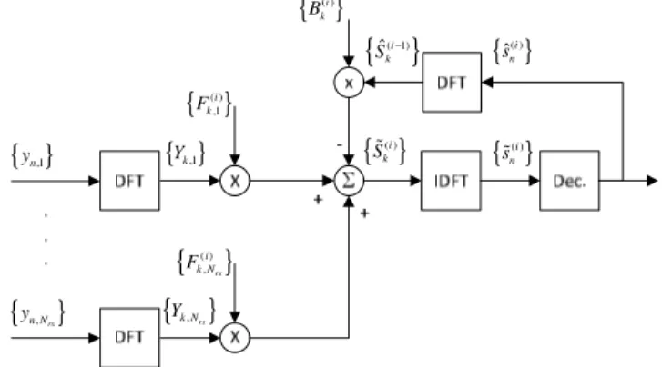
The structure of the iterative receiver which is a direct extension of the IBDFE proposed in [1] with several receive antennas (and similar to the one presented in [11] for only one user) is shown in Fig. 1. It assumes the use of a SC transmission where each block of N modulated symbols, sn, (n=1,…, N), is appended with a suitable cyclic prefix (CP) which is then removed at the receiver. Considering the presence of NI interferers and the use of Nrx receiver antennas, the sequence of received samples after the N-point DFT (Discrete Fourier Transform) block can be written as
= I I
k kSk+ k k+ k
Y H H S N (1)
where Yk is a Nrx×1 vector containing the samples for the kth subcarrier received in the Nrx antennas, Hk is the Nrx×1 vector containing the frequency domain channel coefficients for the different receive antennas, Sk is the kth DFT sample of the main user’s modulated symbols, I
k
H is the Nrx×NI matrix whose entries correspond to the frequency domain channel coefficients for the NI interferers in the different receive antennas (one column for each interferer), I
k
S is the NI ×1 vector whose elements are the kth DFT samples of the different interferers symbols and Nk is the Nrx×1 vector containing noise samples in the frequency domain. It is assumed that both Sk, and Nk are zero mean complex random variables with variances PS =E S k2 and
2
0
N k
P =E N =N N⋅ (N0 is the noise power spectral density). The elements of the interferers’ vector I
k
S are also assumed to be zero mean complex random variables with
( )
I
H
I I
k k S N
ES S = PI . According to Fig. 1, the estimates produced by the IBDFE in the frequency domain for iteration i (from a total a Q iterations) can be expressed as
( ) ( ) ( )ˆ( 1)
= ,
i i i i
k k k k k
Sɶ F Y −B S − (2) where Fk represents a 1×Nrx vector containing the feedforward coefficients for subcarrier k, Bk is the respective feedback coefficient and ˆ(i1)
k
S − is the kth DFT sample of the estimated block ˆ(i 1)
n
s − (n=1,…, N) from the previous iteration after the decision device. { }Yk,1 { }( ) ,1 i k F { }( )i k B
{ }
( )i k Sɶ { }ˆ( )i n s { }( )i n sɶ{
ˆ( 1)i}
k S − { }yn,1{
Yk N,rx}
{
( )}
,rx i k N F{
yn N,rx}
Fig. 1. IBDFE Receiver Structure.
III. OPTIMIZATION FOR INTERFERENCE REJECTION
In this section we will derive the feedforward and feedback coefficients that allow optimum combining of the received signals in the presence of interferers and minimize the MSE between the estimated symbols and the transmitted symbols at the detection point of the receiver. The expressions for computation of the coefficients are then simplified in order to reduce the complexity of the receiver after the first iteration. A. Derivation of IBDFE Coefficients
Let us first we express the MSE as
1 2 ( ) 0 1 N i n n k n MSE E s s N − = = −
∑
ɶ H{
}
1 2 ( ) ( )* 2 0 1 2 Real N i i k k S k k k k E S P E S S N − = = + − ∑
ɶ H ɶ H (3) with( )
2 2 ( ) ( ) ( ) ( ) ˆ H i i H i i k k k k k k k k S E S = E + B P ɶ H F Y Y H F{
( )* ( ) ˆ( 1)*}
2 Real i i i k k k k k k B E S S − − F H H , (4)( )
H H H I I k k k S k k S k k N N EY Y H = PH H +P EH H +P I , (5) and( )
( )*i ˆ H ( )i H ( )*i ˆ(i 1)* k k k S k k k k k k E Sɶ S H =PH F −B E S S − H (6) (throughout this paper (.)*denotes the complex conjugate and (.)H denotes conjugate transpose). The coefficients Fk and Bk that minimize (3) are found under the constraint that the feedback component does not remove the desired signal component [1], i.e., 1 ( ) 0 0 N i k k B − = =∑
. (7) The minimization can then be achieved with the Lagrange multipliers method using the function(
( ) ( ) ( ))
( )* 1 ( ) 0 , , Re N i i i i i k k k k B λ MSE λ B − = Ψ = + ∑
F (8)where λ is the Lagrange multiplier and Re{} denotes the real part. As this function is real valued with complex variables, its minimum can be found using
(
)
(
)
(
)
(
)
* * ( ) ( ) ( ) ( ) ( ) ( ) ( ) ( ) ( ) * , , ( ) ( ) ( ) * , , 0 , , , , 0 0 , , 0 H k k i i i k k H k i i i k k i i i k k B k i i i k k B B B B B λ λ λ λ λ λ ∂Ψ = ∂ ∂Ψ ∇ Ψ = ⇔ = ∂ ∂Ψ = ∂ F F F F F F (9) which leads to(
)
(
)
( )
1 2 ( ) ( ) ( 1) 1 H i i H i H I I N k k k k k k N S P E P γ ρ − − = − + + F H H H H H I (10) and(
)
( 1)* ( ) ( ) ˆ ˆ 1 i k k k i i k k k S E S S B P − = F H − H . (11) In (10), ρ(i−1) is defined as ( 1)* ( 1) ˆ ˆ ˆ . i k k k i S S E S S H P P ρ − − = (12)which can be regarded as a measure of the reliability of the data estimates used in the feedback loop, and γ is selected ( )i
so as to ensure that 1 ( ) 0 1 1 N i k k k N − = =
∑
F H , (13) (i.e., to fulfill condition (7)). Concerning the expected value( )
HI I
k k
E H H in (10), it must be computed over a time period much lower than the reciprocal of the channel fading rate [15]. In this paper we assume perfect knowledge of the interference plus noise covariance matrix at each transmission block (estimation techniques for a real system like LTE can be found in [16][17]).
It is important to note that in the first iteration of the proposed IBDFE we have Bk=0 and
( )
1 (1) (1) H H I I H N k k k k k k N S P E P γ − = + + F H H H H H I (14)which corresponds to a linear IRC detector. Regarding the feedback symbols ˆ( )i
n
s , we can employ soft decisions and compute them using
(
)
( ) ( ) ( ) ˆni E n ni n ni s s s s s p s s s ∈Λ = ɶ =∑
⋅ = ɶ , (15) with Λ representing the set of constellation symbols and(
( )i)
n n
p s =s sɶ corresponding to the probability of the correct symbol sn being s conditioned on the equalizer output sɶ . n
From (2), it is simple to verify that sɶ can be written as n
( )i ( )i
n n n
sɶ =s +ξ , (16) where ( )i
n
ξ represents noise and interference (cochannel and ISI). We can approximate ( )i
n
ξ as a zero mean complex
Gaussian random variable [8] and estimate its variance using
(
( ))
2 1 ( ) ( ) 2 0 1 2 , N i i i n n n s s N ξ σ = − = −∑
⌢ ɶ (17) with ( )i ns⌢ representing the hard decision symbol. The probability
(
( )i)
n n
p s =s sɶ can then be expressed as
(
)
2 ( ) 2( ) 2 ( ) i n i s s i n n p s s s Ke σξ − − = = ɶ ɶ , (18)where K is a normalizing constant. For the particular case of quadrature phase shift keying (QPSK) modulation, and after some manipulations, we can rewrite (15) as
( ) 1 2 ˆ tanh tanh 2 2 2 I Q i S n n n P s j N λ λ = + ⋅ , (19) with I n λ and Q n
λ representing the in-phase and quadrature log likelihood ratios (LLRs), respectively. These LLR are given by
{ }
{ }
( ) ( ) ( ) ( ) 2 Re 1 2 2 2 Im 1 2 2 i n I S n i i n Q S n i s P N s P N ξ ξ λ σ λ σ = = ɶ ɶ , (20)where Im{} denotes the imaginary part. From (19) we can obtain an estimate for ˆ(i 1)*
k k k E S S − H using 1 ( 1)* 0 1 ˆ tanh tanh 2 2 2 I Q N n n i S k k k n P E S S j N λ λ − − = = + ⋅
∑
H . (21)It is possible to extend the application of the receiver to other constellations. In this case E S Sk ˆk(i1)* k
−
H can be estimated following a similar approach to the one described in [20].
B. Simplified Computation of Equalizer Coefficients
Due to ρ(i−1)changing along the iterations, the computation
of the feedforward coefficients using (10) would require a new matrix inversion in every iteration. However the matrix inversion can be avoided after the first iteration by exploiting the Sherman-Morrison identity [21]. Defining the interference plus noise covariance matrix as
( )
= I I H N k k k N S P E P + Φ H H I (22)we can apply the Sherman-Morrison formula and write the matrix inverse in (10) as
(
)
(
)
(
2)
1 ( 1) 1 i H k ρ k k − − + − Φ H H(
)
(
)
(
)
(
)
2 1 1 ( 1) 1 2 1 ( 1) 1 1 1 H i k k k k k H i k k k ρ ρ − − − − − − − = − + − Φ H H Φ Φ H Φ H . (23)Combining (23) with (10),(11),(13) and after some manipulations we can express the feedforward coefficients as
(
)
(
)
( ) ( ) 2 ( 1) 1 1 i i k k i k γ φ ρ − = + − F Γ (24)the feedback coefficients as
(
)
(
)
( 1)* ( ) ( ) 2 ( 1) ˆ ˆ 1 1 1 i k k k i i k k i S k E S S B P φ γ φ ρ − − = − + − H , (25)and the normalizing parameter as
(
)
(
)
( ) 1 2 ( 1) 01 1 i N k i k k N γ φ φ ρ − − = = + −∑
, (26) where 1 H k k k − = Γ H Φ , (27) and k k k φ = Γ H (28) Although Γk depends on a matrix inversion, it only has to be computed once. After the first iteration the computation of( )i
k k
F Y requires only the multiplication of the scalar Γ Yk k by the update scalar ( )
(
(
( 1))
2)
1 1
i i
k
γ +φ − ρ −
which also allows
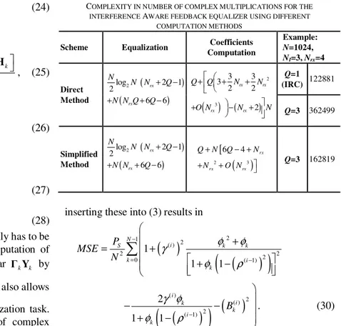
a small reduction in the complexity of the equalization task. Table I compares the complexity in number of complex multiplications of the interference aware IBDFE implemented using both the direct and simplified coefficients computation methods. The ‘Equalization’ column includes the complexity of the signal processing performed by the iterative receiver and the computation of the feedback symbols while the ‘Coefficients Computation’ column includes the complexity associated with ( )i
k
F , ( )i k
B and γ . We have considered that ( )i
the complexity associated with an N-point DFT/IDFT is
(
N 2 log)
2N and with the inversion of an Nrx×Nrx matrix is O(Nrx). In the last column of Table I are shown the number of multiplications for the case of N=1024, NI=3, Nrx=4 and it is possible to observe that while the interference aware IBDFE using a direct implementation results in about 195% of extra complexity over the IRC, the simplified computation method only requires about 32% more which is a substantial reduction.IV. PERFORMANCE ANALYSIS
According to (16), the output of the IBDFE can be represented as the sum of the original symbol with a noise plus interference component. Using the Gaussian approximation for ( )i
n
ξ , the BER dependent on a channel realization for QPSK modulation with Gray mapping can be written as
2 b b E P Q MSE ≈ , (29) with
( )
2 2 1 2 , 0 t x Q x π e dt x ∞ −=
∫
≥ and Eb being the average bit energy. Combining (22), (24), (27), (28) with (4)-(6) andTABLE I.
COMPLEXITY IN NUMBER OF COMPLEX MULTIPLICATIONS FOR THE INTERFERENCE AWARE FEEDBACK EQUALIZER USING DIFFERENT
COMPUTATION METHODS
Scheme Equalization Coefficients
Computation Example: N=1024, NI=3, Nrx=4 Direct Method ( ) ( ) 2 log 2 1 2 6 6 rx rx N N N Q N N Q Q + − + + −
(
)
( ) 2 3 3 3 3 2 2 2 rx rx rx rx Q Q N N O N N N + + + + − + Q=1 (IRC) 122881 Q=3 362499 Simplified Method ( ) ( ) 2 log 2 1 2 6 6 rx rx N N N Q N N Q + − + + − [(
)
2 3 6 4 rx rx rx Q N Q N N O N + − + + + Q=3 162819inserting these into (3) results in
( )
(
)
(
)
2 1 2 ( ) 2 2 2 0 ( 1) 1 1 1 N i S k k k i k P MSE N φ φ γ φ ρ − = − + = + + − ∑
(
)
(
)
(
)
( ) 2 ( ) 2 ( 1) 2 1 1 i i k k i k B γ φ φ ρ − − − + − . (30)It is often interesting to be able to compare the performance of the IBDFE with an ideal one where the feedback symbols are error free, i.e., ˆ(i 1)
k k
S − =S . In this case, inserting (25) and (26)into (30) and noting that ˆ(i 1)*
k k k S E S S − H = P and ( 1) 1 i ρ − =
, allow us to reduce the expression to
1 2 1 0 0 N S k N k k k P MSE φ φ − − = = =
∑
∑
(31)Expressions (29), (30) and (31) can also be used to obtain the BER performance of the conventional linear FDE and IBDFE (described in [10]) which deal with the cochannel interference as additional thermal noise. In this case matrix
k Φ must be defined as
(
1)
= diag ... ... rx k β βl βN Φ (32)where diag(v) denotes a diagonal matrix whose elements correspond to the components of vector v. These elements, βl (l=1,…, Nrx), represent the inverse of the signal to interference plus noise ratio (SINR) in each receive antenna l and can be computed using 2 , , 1 I N I N l k l i i S P E H P β = =
∑
+ , (33) where I, , 2 k l iE H is the channel variance of the ith interferer in the lth antenna and kth subcarrier.
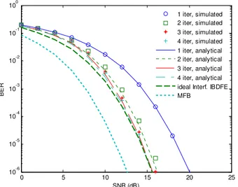
Fig. 2. Analytical and simulated BER performance of the interference aware IBDFE. (Nrx=2, NI=1 with IoT=12dB).
Fig. 3. SNR gain relative to the conventional linear MMSE as a function of the time window (normalized over the reciprocal of the channel fading rate) over which I
( )
I Hk k
E H H is computed. (target BER of 10-4, N
rx=2, NI=1 with
IoT=12dB).
V. PERFORMANCE RESULTS
In order to evaluate the performance of the proposed receiver, Fig. 2 presents analytical and simulated BER performances as a function of the signal to noise ratio (SNR) per antenna for an uncoded SC transmission with N=1024, a block duration of 67µs, a CP with 16.7µs and QPSK modulation. The channel model adopted was the Extended Typical Urban model (ETU) [22] with Rayleigh fading employed in the different taps (similar conclusions could be drawn for other severely time-dispersive channels with rich multipath propagation). Hk, I
( )
I Hk k
E H H and N0 were assumed to be perfectly estimated at the receiver. One interferer contributing with an interference over thermal (IoT) level of 12dB was considered and two receive antennas sufficiently spaced apart so that they can be assumed uncorrelated were used. As a reference we also include in the graph the MFB and the curve of the ideal interference aware
Fig. 4. BER performance of the interference aware IBDFE with several antennas. (NI=1 with IoT =12dB, 3 iterations).
Fig. 5. BER performance of the interference aware IB-FDE with several interferers. (Nrx=4, each interferer contributes with an IoT of 6dB).
IBDFE. It is visible in the figure that the analytical results are very close to the simulated ones. Furthermore, we can also see that the interference aware IBDFE is able to achieve a substantial performance improvement over the linear IRC (IBDFE with 1 iteration). The largest gains are attained after the first 3 iterations which enables the performance curve to become close to the ideal IBDFE for low BERs and with a loss of only about 3dB from the MFB (which does not include multiuser interference nor ISI).
Fig. 3 assumes the same conditions of Fig. 2 but presents the SNR gain relative to the conventional linear MMSE for a target BER of 10-4 as a function of the time window (normalized over the reciprocal of the channel fading rate) over which I
( )
I Hk k
E H H is computed. It is visible that both the interference aware IBDFE and the linear IRC achieve the best performances when the expected value is taken over a period much less than the reciprocal of the fading rate. In this case, the interference aware IBDFE not only has a substantially better performance than the linear IRC, it is also
0 5 10 15 20 25 10-6 10-5 10-4 10-3 10-2 10-1 100 SNR (dB) B E R 1 iter, simulated 2 iter, simulated 3 iter, simulated 4 iter, simulated 1 iter, analytical 2 iter, analytical 3 iter, analytical 4 iter, analytical ideal Interf. IBDFE MFB 10-4 10-2 100 102 104 0 2 4 6 8 10 12 Averaging Window S N R g a in ( d B ) Linear IRC Interf. IBDFE (3 iter.) Conv. IBDFE (3 iter.)
0 5 10 15 20 25 30 10-6 10-5 10-4 10-3 10-2 10-1 100 SNR (dB) B E R _____ N rx=2 ⋅⋅⋅⋅⋅⋅⋅⋅⋅ Nrx=4 ___ N rx=8
° - Conv. linear FDE
∇ - Conv. IBDFE (3 iter.)
∗ - Linear IRC
• - Interf. IBDFE (3 iter.)
0 2 4 6 8 10 12 14 16 18 10-6 10-5 10-4 10-3 10-2 10-1 100 SNR (dB) B E R _____ N I=0 ⋅⋅⋅⋅⋅⋅⋅⋅⋅ NI=1 ___ N I=2 _ ⋅_⋅ NI=3 NI=4 ° - Linear IRC
able to achieve an improvement over the conventional IBDFE receiver which is greater than the one achieved by the linear IRC over the linear MMSE. When the averaging window becomes longer, the performance of both receivers worsens significantly due to the interference on the different antennas being seen as uncorrelated (thus handled as additional thermal noise). In this case they become equivalent to the respective conventional receivers.
In Fig. 4 it is shown the impact of the number of receive antennas for the same conditions of Fig. 3. Only the curves for the linear receivers and IBDFEs with 3 iterations are included. As expected, increasing the number of receive antennas improves the performance of all the receivers (although the gradients increase only slightly due to the already high diversity gain achieved in the adopted frequency selective channel). Furthermore it also lessens the gains provided by the iterative receivers over the linear ones due to the additional diversity which reduces the negative impact of both the ISI and the interferer. However, even with several antennas, the gains provided by the IBDFE over the linear IRC can become quite substantial when the interference increases. This behavior is illustrated in Fig. 5 where the impact of different numbers of interferers is presented when 4 receive antennas are used. It is clearly visible the large gain achieved by the IBDFE when 3 or even 4 interferers are present.
VI. CONCLUSIONS
In this paper we have proposed an IBDFE for SC transmissions whose feedforward and feedback filters are designed with the aim of minimizing the MSE in the presence of cochannel interference, which is often correlated between the receiving antennas. A simplified method for the computation of the filters coefficients which allows reduced complexity after the first iteration was described. Analytical BER expressions were derived and it was shown that the proposed receiver achieves substantial performance gains over the conventional IBDFE and linear IRC detector in severely time dispersive channels with strong cochannel interference levels.
REFERENCES
[1] L.Cimini, ”Analysis and Simulation of a Digital Mobile Channel using Orthogonal Frequency Division Multiplexing,” IEEE Trans. on Comm., Vol. 33, No. 7, July 1985.
[2] D. Falconer, S.L. Ariyavisitakul, A. Benyamin-Seeyar, and B. Eidson, “Frequency domain equalization for single-carrier broadband wireless systems,” IEEE Commun. Mag., vol. 40, no. 4, pp. 58–66, Apr. 2002. [3] A. Gusmão, R. Dinis, R. Conceição, and N. Esteves, “Comparison of
two modulation choices for broadband wireless communications,” in Proc. VTC’00—Spring, vol. 2, pp. 1300–1305, Tokyo, Japan, May 2000. [4] "Evolved Universal Terrestrial Radio Access (E-UTRA); Physical
Channels and Modulation, " 3GPP TS 36.211 v11.3.0, June 2013. [5] M. Silva, A. Correia, R. Dinis, N. Souto, J. Silva, “Transmission
Techniques for Emergent Multicast and Broadcast Systems”, CRC Press -Taylor & Francis Group, Boca Raton, 2010.
[6] N. Benvenuto, R. Dinis, D. Falconer, and S. Tomasin, "Single Carrier Modulation With Nonlinear Frequency Domain Equalization: An Idea Whose Time Has Come—Again," Proceedings of the IEEE, Vol. 98, No. 1, pp. 69 - 96, Jan., 2010.
[7] N. Benvenuto and S. Tomasin, “Block iterative DFE for single carrier modulation,” Electron. Lett., vol. 39, no. 19, pp. 1144–1145, Sept. 2002.
[8] N. Benvenuto and S. Tomasin, “Iterative Design and Detection of a DFE in the Frequency Domain,” IEEE Trans. Commun., vol. 53, no. 11, pp. 1867–1875, Nov. 2005.
[9] C. Zhang, Z. Wang, C. Pan, S. Chen and L. Hanzo, "Low-Complexity Iterative Frequency Domain Decision Feedback Equalization," IEEE
Trans. Veh. Technology., vol. 60, no. 3, pp. 1295– 1301, Mar. 2011. [10] F. Amaral, R. Dinis, N. Souto, P. Montezuma, "Approaching the
matched filter bound with Block Transmission Techniques", Trans. On
Emerging Telecommunications Technologies, Vol. 23, No. 1, pp. 76 - 85, January 2012.
[11] R.Dinis, R. Kalbasi, D. Falconer and A. Banihashemi, “Iterative Layered Space-Time Receivers for Single-Carrier Transmission Over Severe Time-Dispersive Channels,” IEEE Communications Letters, vol. 8, no. 9, pp. 579–581, Sep. 2004.
[12] N. Benvenuto, F. Boccardi and G. Carnevale, ” Frequency Domain Realization of Space-Time Receivers in Dispersive Wireless Channels,”
IEEE Trans. on Signal Processing, Vol. 55, No. 1, Jan. 2007.
[13] C. Dong, J. Lin, K. Niu, Z. He, Z. Bie, “Block-Iterative Decision Feedback Equalizer With Noise Prediction for Single-Carrier MIMO Transmission”, IEEE Trans. Veh. Technology, Vol. 61, No.8, pp.3772-3776, Oct. 2012.
[14] G.M. Guvensen, A.O. Yilmaz, "A General Framework for Optimum Iterative Blockwise Equalization of Single Carrier MIMO Systems and Asymptotic Performance Analysis," Communications, IEEE Trans.
Commun., Vol.61, No.2, pp. 609-619, February 2013.
[15] J. Winters, “Optimum combining in digital mobile radio with cochannel interference,”, IEEE Journal on Selected Areas in Communications, vol. 2, no. 4, pp. 528–539, July 1984.
[16] Y. Ohwatari, N. Miki, Y. Sagae and Y. Okumura, “Investigation on Interference Rejection Combining Receiver for Space-Frequency Block Code Transmit Diversity in LTE-Advanced Downlink,” IEEE Trans.
Veh. Technology, vol. -, no. -, pp. -, June 2013.
[17] Y. Léost, M. Abdi, R. Richter and M. Jeschke, “Interference Rejection Combining in LTE Networks,” Bell Labs Technical Journal, vol. 17, no.1, pp. 25-49, June 2012.
[18] F. Tavares, G. Berardinelli, N. H. Mahmood, T. B. Sørensen, P. E. Mogensen, “On the Potential of Interference Rejection Combining in B4G Networks,” in Proc. VTC 2013—Fall, vol. -, pp. -, Las Vegas, USA, Sep. 2013.
[19] “Enhanced performance requirement for LTE User Equipment (UE),” 3GPP TR 36.829 v11.1.0, January 2013.
[20] R. Dinis, P. Montezuma, N. Souto, J. Silva, “Iterative Frequency-Domain Equalization for General Constellations,” in Proc. IEEE Sarnoff
Symp., vol. -, pp. -, Princeton, USA, April 2010.
[21] J. Sherman and W. J. Morrison, “Adjustment of an Inverse Matrix Corresponding to a Change in One Element of a Given Matrix,”, Annals
of Mathematical Statistics, vol. 21, no. 1, pp. 124–127, Mar. 1950. [22] "Evolved Universal Terrestrial Radio Access (E-UTRA); Base Station
(BS) radio transmission and reception, " 3GPP TS 36.104 v11.6.0, Sept. 2013.