Printed version ISSN 0001-3765 / Online version ISSN 1678-2690 http://dx.doi.org/10.1590/0001-3765201720160784
www.scielo.br/aabc | www.fb.com/aabcjournal
Growth of the silverside
Atherinella brasiliensis
in a subtropical estuary
with some insights concerning the weight-length relationship
BARBARA M. DE CARVALHO1
, JOSÉ RICARDO S. BARRADAS2
, NELSON F. FONTOURA2 and HENRY L. SPACH1,3
1
Programa de Pós-Graduação em Zoologia, Departamento de Zoologia, UFPR, Centro Politécnico, Caixa Postal 19020, Jardim das Américas, 81531-980 Curitiba, PR, Brazil
2
Faculdade de Biociências, PUCRS, Av. Ipiranga, 6681, 90619-900 Porto Alegre, RS, Brazil 3
Programa de Pós-Graduação de Sistema Costeiro e Oceânicos, UFPR, Av. Beira-Mar, s/n, Caixa Postal 61, Bal. Pontal do Sul, 83255-976 Pontal do Paraná, PR, Brazil
Manuscript received on November 10, 2016; accepted for publication on March 8, 2017
ABSTRACT
Specimens of Brazilian silverside (Atherinella brasiliensis, n=9672) with a length range of 1.5 to 14.2 cm were captured in the intertidal areas of the Estuarine Complex of Paranaguá, Brazil, between August 2010 and July 2011. The species’ weight-length relationship was represented by the equation W=0.00533 L3.136
with a slightly positive allometry (b>3) and could be divided into two growth stanzas: W = W1 + W2; Stanza 1: W1= SW. (0.005239 L3.152); Stanza 2: W2= (1 – SW). (0.000699 L3.913); Switch-Function: SW = [1 + e1.204 (L – 11.66)]-1. The breakpoint between the first and second stanza (11.66 cm) matches published values
for the estimated size at first maturity of adult females. Frequency distributions indicate that the species
is present in the shallow areas of the Estuarine Complex of Paranaguá during all phases of its ontogenetic development, with the recruitment of juveniles taking place between October and November. Modal
displacement was monitored throughout 12 months. The von Bertalanffy growth model and longevity was estimated as follow: asymptotic length (L∞) of 17.5 cm, growth coefficient (K) of 0.89 (year-1
) and longevity (A95) of 3.33 years. We present some considerations with regard to the general methodology for adjusting weight-length relationships.
Key words: Atherinopsidae, longevity, von Bertalanffy, weight-length relationship.
Correspondence to: Nelson Ferreira Fontoura E-mail: [email protected]
INTRODUCTION
Fish growth patterns are influenced by counteracting driving forces, such as food availability, environmental factors and species requirements during the fish life cycle, e.g. for reproduction, migration or territory defense. By
investing energy to grow faster, fish can avoid
high predation rates of smaller animals. On the
other hand, a focus on early reproduction reduces
expected final size, but increases the chance
of an individual to pass its genes on to the next
generation. Therefore, the success of a species and
its life-history strategy results from interacting
a specific growth pattern could be interpreted as
an indirect result of the selected life strategy. For example, species with a wide geographical range are likely to have latitudinal growth patterns,
with increasing final size and decreasing growth
rates in higher latitudes (Taylor 1958, 1959, 1960, 1962, Pauly 1980, Fontoura and Agostinho 1996, Giacomini and Shuter 2013, Peck et al. 2013).
The family of Atherinopsidae comprises 13 genera and 104 species of marine, estuarine
and freshwater fish, 14 of which occur in Brazil:
Atherina lessoni, Atherinella blackburni, A. brasiliensis, Odontesthes argentinensis, O. bicudo, O. bonariensis, O. incisa, O. humensis, O. ledae, O. perugiae, O. piquava, O. mirinensis, O. retropinnis
and Pseudothyrina iheringi (Froese and Pauly 2017).
Atherinella brasiliensis has the widest geographic distribution of all American Atherinopsidae, ranging from Venezuela (10° N) to southern Brazil (32° S) (Brian and Dyer 2006).
Atherinella brasiliensis is common in estuarine areas, but also occurs in coastal waters (Hostim-Silva et al. 1995, Pessanha and Araújo 2001, Neves et al. 2006, Fávaro et al. 2007). The species has generalist and opportunist feeding habits (Chaves and Vendel 2008, Contente et al. 2010). Estimated
length at first maturity varies from 7.6 to 9.1cm
of total length. Intense reproduction activities take place between October and January (Bervian and Fontoura 1997, Fávaro et al. 2003), involving the deposition of adherent benthic eggs and direct larval development (Del Río et al. 2005). A compilation of published information concerning growth and mortality of the species along the Brazilian coast is presented in Table I. The weight-length relationship is characterized by positive allometric growth. Concerning parameters of the
von Bertalanffy growth curve, asymptotic lengths
are estimated between 11.3 and 17 cm and the growth constant ranging between 0.82-0.89 (year -1
); resulting in longevity estimates of slightly more
than three years (Paiva-Filho and Giannini 1990, Haimovici and Velasco 2000, Pessanha and Araújo 2001, Giarrizzo et al. 2006, Macieira and Joyeux 2008, Mazzei et al. 2011, Freire et al. 2012, Costa et al. 2013, Franco et al. 2013).
In the present study we describe the weight-length relationship and growth patterns of A. brasiliensis within the Estuarine Complex of Paranaguá (Paraná, Brazil), aiming to identify possible latitudinal trends of the species along the Brazilian coast. Also, some considerations with regard to the general methodology for adjusting weight-length relationships are presented.
MATERIALS AND METHODS
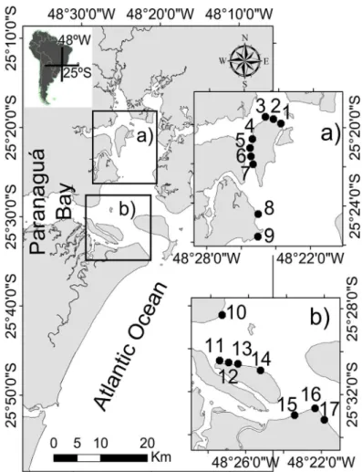
Specimens were collected once a month between August 2010 and July 2011 at 17 sites along the north-south axis in intertidal areas (~1 m, neap tide) of the Estuarine Complex of Paranaguá, Brazil (Fig. 1, 25º 15’ - 25° 35’ S and 48° 20’ - 48° 45’ W) through a 30 m coastal trawling with a beach seine net (15 m long; 2 m high; 2.5 mm mesh) (IBAMA 10.876). After collection, specimens were cooled, identified to species (Menezes and Figueiredo 2000), measured for total length (Lt; 0.01 cm) and weighed (P; 0.01 g).
Weight-length relationship was adjusted by using a power equation (Froese 2006): W = a.Lb, where W is the weight (g), L is the total length (cm), a is the coefficient of proportionality, and b
is the coefficient of allometry. To avoid the bias
TABLE I
Summary of published information concerning growth and longevity parameters of Atherinella brasiliensis along the
Brazilian coast. Lmax is the maximum total length (cm); L∞ and K are the asymptotic length (cm) and growth constant (year-1) according to the von Bertalanffy growth model; a
and b are the proportionality and allometry coefficients of the
weight-length relationship. And (J) means immature individuals, (M) male and (F) female.
Author Latitude Lmax
(cm)
L∞
(cm) K (year
-1
) Longevity
(years) a b
Giarrizzo et al. (2006) 0°10’S 11.4 0.0061 3.03
Freire et al. (2012) 05°46’S 14.9 0.004 3.23
Freire et al. (2012) 14°48’S 13.4 0.005 3.11
Mazzei et al. (2011) 19°57’S 12.36 0.0061 3.01
Macieira and Joyeux (2008) 20°50’S 7.1 0.0072* 2.91
Franco et al. (2013) 22°49’ to 57’S 17.7 0.005 3.01
Pessanha and Araújo (2001) 22°5’ to 23°0’S 11.26 0.930 3.1
Costa et al. (2013) 23°02’S 16.0 0.006 2.97
Paiva-Filho and Giannini (1990) 24°25’S 13.1 0.006* 3.03
Haimovici and Velasco (2000) 28° to 34°S 15.5 0.0033 3.33
Bervian and Fontoura (2007) 29°58’S 17.0 0.0068 (J) 3.03
16.0 0.884 3.4 0.0049 (M) 3.20
17.0 0.825 3.6 0.0049 (F) 3.20
* Length converted to centimeters.
within a single information point, aiming to reduce the natural variability that can hide subtle trends, and (2) by using narrower size classes for small and abundant juveniles, and by increasing
the size interval (on a log scale) for larger fishes
to account for their lower abundance in samples, thus minimizing (but not eliminating) bias from the unbalanced sampling design. To handle intrinsic heteroscedasticity of the weight-length relationship data, a power function was adjusted to the weight standard deviation of each size class: Wsd = asd. Lcbsd, where Wsd is the weight standard deviation for each size class, Lc is average total length of each size class, and asd and bsd are empirical
coefficients. Once a general trend concerning the heteroscedastic pattern was identified, this trend
was used to keep a homoscedastic residual: Rh = (W – West)/(asd.Lcbsd), were Rh is the homocedastic
residual, W is the measured weight of each individual and West is the estimated weight of the weight-length function. Complementary procedures for polyphasic adjustment can be found in Bervian et
al. (2006), Fontoura et al. (2010) and Oliveira et
al. (2011). Detailed scripts for polyphasic fitting
by using R statistical platform could be found in J.R. Barradas (unpublished data; http://repositorio. pucrs.br/dspace/bitstream/10923/8518/3/TES_ JOSE_RICARDO_DE_SOUZA_BARRADAS_ COMPLETO.pdf).
The species life cycle was interpreted by grouping specimens into length-frequency intervals (every other month) to improve visibility concerning the general pattern of modal displacement. Age groups were estimated by taking into account the time gap between each sample and the climax of the annual reproductive period (October in the Bay of Paranaguá; Fávaro et al. 2003). The age of each specimen was assessed according to its age group.
Superimposed age groups were artificially divided
within the crossing edge of both tails.
Size-at-age was described by the von
Bertalanffy (1938) growth curve: Lt = L∞ [1 - e-K.
(t–t0)
], where: Lt is total length (cm) at age t (years),
Figure 1 - Sampling area and sampling sites (black dots). Estuarine Complex of Paranaguá, Brazil.
growth rate, and t0 is a time-correcting factor
related to the size at birth or eclosion. Model
adjustment (SPSS 17.0; nonlinear routine;
Levenberg-Marquardt algorithm) was performed
by using the length to age relationship of all
captured individuals comprising a time series of
the first identified age-group in November/2010;
which was followed to July/2011. As there were
no captures after July/2011, animals that belonged
to this age group (1+) but were captured between
August-November/2010, were used to emulate the
growth pattern of this cohort. Longevity, estimated
as the time a fish takes to reach 95% of L∞, was
calculated as follows: A95= -2.96/K, in which K is
the instantaneous growth rate of the von Bertalanffy
growth model (Taylor 1958, 1959, 1960, 1962). Using the available growth and mortality parameters of A. brasiliensis along the Brazilian coast, linear regressions were applied to identify latitudinal patterns as described in the literature (Taylor 1958, 1959, 1960, 1962, Pauly 1980, Fontoura and Agostinho 1996, Giacomini and Shuter 2013, Peck et al. 2013).
RESULTS
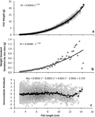
Figure 2a shows the weight-length relationship (W=0.00558 L3.113) for the complete data set (gray dots), as well as the average weight by average length by size class (black dots). Weight standard deviation by size class shows a typical power function pattern (Wsd = 0.00280 L2.198; Fig. 2b), which was used to correct the heteroscedastic pattern to obtain a homoscedastic residual distribution.
Residual distribution from a regular weight-length relationship is presented in Fig. 2c. Although no pattern was detected when analyzing the entire data set (gray dots), a clear trend was apparent for the average weight to average length by size class (black dots) which can be described as an empirical polynomial function (R = 0.0026x4 – 0.0825x3 + 0.895x2 – 3.903x + 5.753; R²=0.589), with notable anomaly regarding animals longer than 10 cm.
By applying a polyphasic model according to Bervian et al. (2006) the growth of A. brasiliensis
could be divided into two stanzas (Fig 3a): Switch-Function: SW = [1 + e1.204 (L – 11.66)]-1 Stanza 1: W1= SW . (0.005239 L3.152) Stanza 2: W2= (1 – SW). (0.000699 L3.913) W = W1 + W2
After adjusting the polyphasic model, no residual pattern could be identified (Fig. 3b; R²=0.00002), indicating that the polyphasic growth model accounted for all of the potentially explained weight variance.
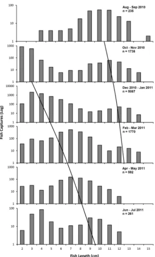
Figure 4 shows the size distribution of A. brasiliensis in the Estuarine Complex of Paranaguá (grouped bimonthly to increase data consistency). The first sampling period (Aug-Sep/2010) was characterized by a modal group in which most individuals were larger than 7 cm (mean Lt = 9.5 ± 1.86 cm), the smallest mature female reported by Bervian and Fontoura (1997), and comprise basically an adult age-group. In the Oct-Nov sample, newborn juveniles with a size range of 2-3 cm appeared and were present throughout the year, although with decreasing abundance, indicating a long recruitment period with increased intensity in October/November. Trend lines are presented in Fig. 4 to suggest modal displacement within the annual cycle.
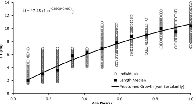
Figure 5 graphs the length of all collected specimens (open dots), month by month for the entire year, with individual age assessed by the length frequency distribution. It also presents the median total length of specimens of the same age (black squares) and the predicted growth curve following von Bertalanffy´s model. Estimated growth parameters are presented in Table II. Longevity (A95) was estimated to be 3.3 years.
Latitudinal patterns in relation to growth and mortality parameters were evaluated by using linear
regression, but with no identifiable trends (P>0.05).
Figure 2 -Atherinella brasiliensis in the Estuarine Complex of Paranaguá, Brazil. White dots represent data of individuals; black dots (or gray in Fig. 1b) represent average length to average weight for size classes: a) weight-length relationship;
DISCUSSION
As observed in the present study, most existing analyses of growth patterns of A. brasiliensis
(Table I) indicate a positive allometric growth, except for the analyses by Macieira and Joyeux (2008), and Costa et al. (2013). As a general trend, a positive allometric growth can be expected for
most fish species (Froese 2006, Froese et al. 2014).
Animals of all sizes were captured throughout the year, suggesting that the species completes its ontogenetic development in the shallow waters of
the study area. The occurrence of all ontogenetic phases of A. brasiliensis in intertidal zones was also observed by Favero and Dias (2015).
An in-depth review (Froese 2006) on the weight-length relationship of fish, and a meta-analysis using Bayesian statistics (Froese et al.
2014) identified general trends of the weight-length
relationship according to body shape. As a general approach they suggested to use Log10 transformed data to linearize the power function of the weight-length relationship.
Both papers, together with the review of Le Cren (1951), are landmarks in the weight-length literature, describing research history, clarifying Figure 3 -Atherinella brasiliensis in the Estuarine Complex
of Paranaguá, Brazil. White dots represent data of individuals; black dots represent average length to average weight for size classes: a) polyphasic weight-length relationship; b) residual distribution from a polyphasic weight-length relationship.
Figure 4 -Atherinella brasiliensis in the Estuarine Complex of Paranaguá, Brazil. Length frequency distribution for samples collected every other month. Diagonal lines are drawn by hand and represent the hypotheses for modal displacement.
TABLE II
Estimated parameters of the von Bertalanffy growth equation of Atherinella brasiliensis of the Estuarine
Complex of Paranaguá, Brazil;K = growth coefficient; to = age when fish have zero theoretical length; L∞ = asymptotic length; Std. Error = standard error; CI =
Confidence Interval.
Parameter Estimate Std. Error 95% CI
K (year-1
) 0.890 0.042 0.806 and 0.973 to (year) -0.060 0.003 -0.067 and -0.054
Figure 5 -Atherinella brasiliensis in the Estuarine Complex of Paranaguá, Brazil. Growth curve according to the von Bertalanffy
growth model.
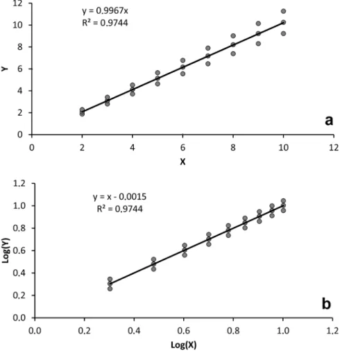
Figure 6 - Bias resulting from adjusting a power function from log-transformed data: a) an artificial data series using the simple power function:
Y = 1. X1, with homoscedastic variability (Y±1). The trend line represents the
concepts, suggesting approaches, and, importantly
proposing general trends concerning fish biology.
Nevertheless, the problems associated with log-transformations to cope with power functions has been pointed out by Smith (1993), and are
highlighted in Figure 6. For Fig. 6a, an artificial data
series was created using the simple power function: Y = 1. X1. We also introduced homoscedastic variability (Y±1) to simulate “real” world data. If a power function is adjusted using standard statistical packages (log-transformation routines), the result is far from a=1 and b=1. In this case, a
was underestimated to 0.899 and b overestimated to 1.05, i.e. a pure isometric data set was estimated as with positive allometry.
Fig. 6b explains the reason for these biases. When values are compressed, lower values undergo less compression than higher values. This is problematic in two ways. Any regression is a balance around a theoretical axis centered between average Y and X values. By compressing X values, the center of balance is downgraded to smaller X values, decreasing the number of individuals below X average. But the major problem is related to the compression of Y values. For each set of values, the Y values above the trend line will be more compressed than Y values below the trend line, and this is especially true for small animals. This unbalanced treatment of Y values will lower the trend line for small animals, underestimating presumed weight, and increase the weight of large animals, overestimating their presumed weight. As a mathematical “trap”, the trend line rotates counter-clockwise, decreasing the proportionality coefficient (a) and increasing the allometric coefficient (b). This second problem occurs especially with small samples and large weight variability.
Of course, these biases are amplified in the
present simulation due to artificially increased variability for small animals. Fortunately, with real
fish data, this is less of a problem since absolute
variability of small animals is usually narrow (see Fig. 7). Here, we used variability that was more similar to real data (heterocedastic; Y± Y/10). In this case, Log10 transformation brings the data to a homoscedastic pattern, although with an unbalanced compression of Y values above and below the adjusted trend line. In this simulation, however, the estimated allometry (b value) is correctly estimated as 1.0, although with some distortion concerning proportionality (0.9967 instead of 1.0), but with no practical implication.
By using the entire data set of A. brasiliensis
and by fitting a regular weight-length relationship
with non-linear adjustment, our estimate for b was 3.136, and was very similar when log-transformed data (b=3.139) were used, with no practical
difference regarding proportionality. If the general
recommendations of Froese (2006) are followed with good quality data, bias should be minimal.
Thus, although we argue that nonlinear algorithms are, in theory, better tools for the adjustment of weight-length relationships, the application of linear regression to log-transformed
data is sufficient for general use. In particular, the allometry coefficient appears not to be severely
compromised by data transformation and the general patterns described by Froese et al. (2014) are probably very close to real patterns.
With regard to the polyphasic weight-length relationship, our intention was to supply information that can elucidate details of the species’ life-history instead of simply describing a useful
tool for fishery management. The objective is not
the weight-length relationship itself, but to use weight-length information to examine the species’ biology.
For A. brasiliensis the weight-length
relationship can be divided in two stanzas. The first
stanza, with b=3.152, describes the weight-length relationship of animals up to 11.66 cm. Above this size, the b value increases to 3.913. The transition
a switch function at a relatively slow rate (1.204) with no strong disruption of the growth pattern. The
side effect is that the proportionality and allometry coefficients of the second stanza are mathematical artifacts, resulting from the “tail” of the first stanza
(Fig. 3a).
Although this general methodology is an interesting tool to describe the growth pattern for
each specific stanza, as in Bervian et al. (2006),
Fontoura et al.(2010) and Oliveira et al. (2011), it sets the potential trap of achieving a good statistical result with little biological meaning. But the
benefit of this approach does not lie in the stanzas
themselves, but in identifying the breakpoint between stanzas, that could indicate an interesting shift in the species’ life-cycle. Concerning A. brasiliensis, the breakpoint (11.6) is the size
estimated by Fávaro et al. (2003) for 100% of the
females at sexual maturity in the Paranaguá estuary. While this information is already available, the key point here is to identify whether the reproductive
cycle is imprinted in the growth patterns of fish
(Bervian et al. 2006, Fontoura et al.2010, Oliveira et al. 2011).
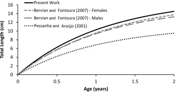
The adjusted von Berfalanffy growth model (L∞ = 17.45; K= 0.89; Paranguá; 25°S) was
Figure 7 - Bias resulting from adjusting a power function from log-transformed data: a)
an artificial data series using the simple power function: Y = 1. X1
, with heteroscedastic
similar to estimated models published by Bervian
and Fontoura (2007; Females: L∞=17.0; K=0.825; Males: L∞=16.0; K=0.884; Tramandaí; 29°S) and the FishBase life history tool (L∞=17.0; K=0.83).
On the other hand, Pessanha and Araújo (2001; Sepetiba Bay, 23°S) estimated a larger growth
constant (K=0.93) but a smaller asymptotic length (L∞ = 11.26), resulting in a reduced growth pattern
(Fig. 8).
Although a smaller total size is expected for lower latitudes as described by Taylor (1958, 1959,
1960, 1962), latitudinal differences did not explain the identified pattern. The length-frequency data
of Pessanha and Araújo (2001) indicates that very few animals were captured with total length > 10 cm (the largest animal was 13.8 cm). Also, there
is a difference in sampling methods: the present
work and Bervian and Fontoura (2007) used a 15 m long beach seine net, while Pessanha and Araújo (2001) used a 10 m long seine net. Although the escape capacity of larger animals is unknown, the lack of larger animals in Sepetiba bay may be due to sampling bias, since animals up to 16 cm length
have been reported for the same latitude (Costa et al. 2013).
An estimated life span of 3.3 years is very similar to the one proposed by Bervian and Fontoura (2007; Males; A95=3.4; Females; A95=3.6) and that of the FishBase Life history tool (3.4 years). Nevertheless, very few individuals in a size
compatible with a two year old fish (≈14 cm) and
none with size in size predicted for three year old
fish (≈16cm) were captured, although animals of
this size have been reported in literature (Table I). Especially, no animal was captured with lengths larger than 12 cm after April, suggesting that a displacement of large animals to deeper waters may be happening.
Considering that ten different estimates of the weight-length relationship of A. brasiliensis
are available (Table I), we also intended to test the hypothesis of a latitudinal trend concerning proportionality and allometry coefficients, as expected for maximum length (Taylor 1958, 1959,
1960, 1962). Nevertheless, no trend was identified,
Figure 8 -Atherinella brasiliensis in the Estuarine Complex of Paranaguá, Brazil. Growth curve according to the
von Bertalanffy growth model compared to published models (Pessanha and Araújo 2001, Bervian and Fontoura
possibly due to a nonexisting trend or to poor data quality.
Finally, growth studies of fish species are still
needed, since growth parameters for most species are unknown. Also, a meta-analytical approach is highly recommended to summarize growth patterns in relation to environmental gradients (Taylor 1958, 1959, 1960, 1962, Pauly 1980), body shape (Froese et al. 2014) and phylogenetic driving forces (Rodrigues et al. 2014).
ACKNOWLEDGMENTS
The authors would like to thank Coordenação de Aperfeiçoamento de Pessoal de Nível Superior (CAPES) for the scholarship awarded to Barbara Maichak de Carvalho and José Ricardo de S. Barradas (M.SC and PhD scholarships) and
Conselho Nacional de Desenvolvimento Científico
e Tecnológico (CNPq) for the scholarship awarded to Nelson Ferreira Fontoura (research scholarship).
REFERENCES
BERVIAN G AND FONTOURA NF. 1997. Reprodução de
Atherinella brasiliensis no estuário do rio Tramandaí, Imbé, Rio Grande do Sul, Brasil (Teleostei, Atherinopsidae). Biociências 5: 19-32.
BERVIAN G AND FONTOURA NF. 2007. Growth of the Silverside Atherinella brasiliensis in Tramandaí Estuary, Southern Brazil (Actinopterygii: Atherinopsidae). Neotrop Ichthyol 5: 485-490.
BERVIAN G, FONTOURA NF AND HAIMOVICI M. 2006. Statistical model of variable allometric growth: otolith growth in Micropogonias furnieri (Actinopterygii, Sciaenidae). J Fish Biol 68: 196-208.
BRIAN S AND DYER H. 2006. Systematic revision of the South American silversides (Teleostei, Atheriniformes). Biocell 30: 69-88.
CHAVES PT AND VENDEL AL. 2008. Análise comparativa da alimentação de peixes (Teleostei) entre ambientes de marisma e de manguezal num estuário do sul do Brasil (Baía de Guaratuba, Paraná). Rev Bras Zool 25: 10-15. CONTENTE RF, STEFANONI MF AND SPACH HL. 2010.
Feeding ecology of the Brazilian silverside Atherinella brasiliensis (Atherinopsidae) in a sub-tropical estuarine
ecosystem. J Mar Biol Assoc UK 91: 1197-1205.
COSTA MR, PEREIRA HH, NEVES LM AND ARAÚJO FG. 2013. Length–weight relationships of 23 fish species from Southeastern Brazil. J Appl Ichthyol 30: 1-3.
DEL RÍO V, ROSAS J, VELÁSQUEZ A AND CABRERA T. 2005. Desarrollo embrionário larval y tiempo de metamorfoses del pez tropical Xenomelaniris brasiliensis
(Pisces: Atherinidae). Rev Biol Trop 53: 1-10.
FÁVARO LF, LOPES SCG AND SPACH HL. 2003. Reprodução do peixe-rei, Atherinella brasiliensis (Quoy & Gaimard) (Atheriniformes, Atherinidae), em uma planície de maré adjacente à gamboa do Baguaçu, Baía de Paranaguá, Paraná, Brasil. Rev Bras Zool 20: 501-506. FÁVARO LF, OLIVEIRA EC AND VERANI NF. 2007.
Estrutura da população e aspectos reprodutivos do peixe - rei Atherinella brasiliensis (Quoy & Gaimard) (Atheriniformes, Atherinopsidae) em áreas rasas do Complexo Estuarino de Paranaguá, Paraná, Brasil. Rev Bras Zool 24: 1150-1156.
FAVERO JM AND DIAS JF. 2015. Juvenile fish use of the shallow zone of beaches of the Cananéia-Iguape coastal system, southeastern Brazil. Braz J Oceanogr 63: 103-114. FONTOURA NF AND AGOSTINHO AA. 1996. Growth with
seasonally varying temperatures: an expansion of the von Bertalanffy growth model. J Fish Biol 48: 569-584. FONTOURA NF, JESUS AS, LARRE GG AND PORTO JR.
2010. Can weight/length relationship predict size at first maturity? A case study with two species of Characidae. Neotrop Ichthyol 8: 835-840.
FRANCO TP, ARAÚJO CEO AND ARAÚJO FG. 2013. Length–weight relationships for 25 fish species from three coastal lagoons in Southeastern Brazil. J Appl Ichthyol 30: 1-3.
FREIRE KMF, NASCIMENTO FP, ROSÁRIO LMO, ROCHA
GRA, ALVES GA AND LINS-OLIVEIRA JE. 2012. Characterization of some biological aspects of Atherinella brasiliensis caught during sport fishing tournaments: a case study from Northeastern Brazil. Bol Inst Pesca 38: 171-180.
FROESE R. 2006. Cube law, condition factor and weight– length relationships: history, meta-analysis and recommendations. J Appl Ichthyol 22: 241-253.
FROESE R AND PAULY D (Eds). 2017. FishBase. World Wide Web electronic publication. <www.fishbase.org>, version (01/2017).
FROESE R, THORSON JT AND REYES JR RB. 2014. A Bayesian approach for estimating length-weight relationships in fishes. J Appl Ichthyol 30: 78-85.
GIACOMINI HC AND SHUTER BJ. 2013. Adaptive responses of energy storage and fish life histories to climatic gradients. J Theor Biol 339: 100-111.
fish fauna in a mangrove estuary in Northern Brazil. J Appl Ichthyol 22: 325-327.
HAIMOVICI M AND VELASCO G. 2000. Length weight relationships of marine bony fishes from Southern Brazil. Naga 23: 19-23.
HOSTIM-SILVA M, CLEZAR L, RIBEIRO GC AND MACHADO C. 1995. Estrutura populacional de
Xenomelaniris brasiliensis (Quoy & Gaimard, 1824) na Lagoa da Conceição, SC. Braz Arch Biol Technol 38: 949-960.
LE CREN ED. 1951. The length – weight relationship and season cicle in gonad weight and codition in the perch (Perca fluviatilis). Freshwater Biol Association 20: 201-219.
MACIEIRA RM AND JOYEUX JC. 2008. Length–weight relationships for rockpool fishes in Brazil. J Appl Ichthyol 24: 1-2.
MAZZEI E, JOYEUX JC AND SIMON T. 2011. Length– weight relationships for juvenile and small-sized adult fishes of the surf zone. J Appl Ichthyol 27: 1137-1138. MENEZES NA AND FIGUEIREDO JL. 2000. Manual de
peixe marinhos do sudeste do Brasil Teleostei I. Museu de Zoologia, Universidade de São Paulo, p. 1-101.
NEVES ML, PEREIRA HH, COSTA RM AND ARAÚJO GF. 2006. Uso do manguezal de Guaratuba, Baia de Sepetiba, Rio de Janeiro, pelo peixe-rei Atherinella brasiliensis
(Quoy & Gaimard) (Atheriniformes, Atherinopsidae). Rev Bras Zool 23: 421-428.
OLIVEIRA VA, FONTOURA NF AND MONTAG LFA. 2011. Reproductive characteristics and the weight-length relationship in Anableps anableps (Linnaeus, 1758) (Cyprinodontiformes: Anablepidae) from the Amazon Estuary. Neotrop Ichthyol 9: 757-766.
PAIVA-FILHO AM AND GIANNINI R. 1990. Contribuição ao conhecimento da biologia do peixe-rei, Xenomelaniris
brasiliensis (Quoy & Gaimard, 1824) (Atherinidae), no complexo baía-estuário de Santos e São Vicente, Brasil. Bol Inst Oceanogr 38: 1-9.
PAULY D. 1980. On the interrelationships between natural mortality, growth parameters, and mean environmental temperatures in 175 fish stocks. J Cons Int Explor Mer 39: 175-192.
PECK MA, REGLERO P, TAKAHASK M AND CATALÁN
IA. 2013. Life cycle ecophysiology of small pelagic fish and climate-driven changes in populations. Progr Oceanogr 116: 220-245.
PESSANHA ALM AND ARAÚJO FG. 2001. Recrutamento do peixe-rei, Atherinella brasiliensis (Quoy & Gaimard) (Atheriniformes, Atherinopsidae), na margem continental da Baía de Sepetiba, Rio de Janeiro, Brasil. Rev Bras Zool 18: 1265-1274.
RODRIGUES LHR, FONTOURA NF AND MARQUES DM. 2014. Food-web structure in a subtropical coastal lake: how phylogenetic constraints may affect species linkages.Mar Fresh Res 65: 453-465.
SMITH RJ. 1993. Logarithmic transformation bias in allometry. Am J Phys Anthrop 90: 215-228.
TAYLOR CC. 1958. Cod growth and temperature. J Cons Int Explor Mer 23: 366-370.
TAYLOR CC. 1959. Temperature and growth - the Pacific razor clam. J Cons Int Explor Mer 25: 93-101.
TAYLOR CC. 1960. Temperature, growth and mortality - the Pacific cockle. J Cons Int Explor Mer 26: 117-124. TAYLOR CC. 1962. Growth equations with metabolic
parameters. J Cons Int Explor Mer 27: 270-286.