1 Copyright © #### by ASME
“CLASSIFICATION OF RECORDED CLASSICAL MUSIC
USING NEURAL NETWORKS”
R. Malheiro
abR. P. Paiva
bA. J. Mendes
bT. Mendes
bA. Cardoso
b aESCT – Escola Superior de Ciências e Tecnologia da Universidade Católica PortuguesaCentro Regional das Beiras - Viseu,
Estrada da Circunvalação, P 3504-505, Viseu, Portugal
Tel. +351-232-419500, Fax: +351-232-428344, e-mail: [email protected]
bCISUC – Centro de Informática e Sistemas da Universidade de Coimbra
Departamento de Engenharia Informática, PÓLO II da Universidade de Coimbra, Pinhal de Marrocos, P 3030, Coimbra, Portugal
Tel. +351-239-790000, Fax: +351-239-701266, e-mail: {ruipedro, toze, tmendes, amilcar}@dei.uc.pt
Abstract
As a result of recent technological innovations, there has been a tremendous growth in the Electronic Music Distribution industry. In this way, tasks such us automatic music genre classification appear as new and exciting research challenges.
Automatic music genre recognition involves issues like feature extraction and development of classifiers using the obtained features.
As for feature extraction, we use the number of zero crossings, loudness, spectral centroid, bandwidth and uniformity. These features are statistically manipulated, making a total of 40 features.
Regarding the task of genre modeling, we train a feedforward neural network (FFNN) with the Levenberg-Marquardt algorithm.
A taxonomy of subgenres of classical music is used. We consider three classification problems: in the first one, we aim to discriminate between music for flute, piano and violin; in the second problem, we distinguish choral music from opera; finally, in the third one, we aim to discriminate between all the abovementioned five genres together.
We obtained 85% classification accuracy in the three-class problem, 90% in the two-class problem and 76% in the five-class problem. These results are encouraging and show that the presented methodology may be a good starting point for addressing more challenging tasks.
Keywords: neural networks, music information
retrieval, music classification, music signal analysis1. Introduction
Presently, whether it is the case of a digital music library, the Internet or any music database, search and retrieval is carried out mostly in a textual manner, based on categories such as author, title or genre. This approach leads to a certain number of difficulties for service providers, namely in what concerns music labeling. Real-world music databases from sites like AllMusicGuide or CDNOW grow larger and larger on a daily basis, which requires a tremendous amount of manual work for keeping them updated.
Thus, simplifying the task of music database organization would be an important advance. This calls for automatic classification systems. Such systems should overcome the limitations resulting from manual song labeling, which may be a highly time-consuming and subjective task.
Some authors have addressed this problem recently. Tzanetakis and Cook [13] classify music in ten genres, namely, classical, country, disco, hip-hop, jazz, rock, blues, reggae, pop and metal. They further classify classical music into choir, orchestra, piano and string quartets. Features used encompass three classes: timbral, rhythmic and pitch-related features. The authors investigate the importance of the features is training statistical pattern recognition classifiers, particularly, Gaussian Mixture Models and k-nearest neighbors. 61% accuracy was achieved for discriminating between the ten classes. As for classical music classification, an average accuracy of 82.25% was achieved. Golub [2] uses seven classes of mixed similarity (a capella, celtic, classical, electronic, jazz, latin and pop-rock). The features used are
loudness, spectral centroid, bandwidth and uniformity, as well as statistical features obtained from them. A generalized linear model, a multi-layer perceptron and a k-nearest classifier were used. The best of them achieved 67% accuracy. Kosina [5] classifies three highly dissimilar classes (metal, dance and classical) using k-nearest neighbors. The used features were mel-frequency cepstral coefficients, zero-crossing rate, energy and beat. 88% accuracy was achieved. Martin [7] addresses the problem of instrument identification. He proposes a set of features related to the physical properties of the instruments with the goal of identifying them in a complex auditory environment.
In our work we aim at classifying five subgenres of classical music, namely, opera, choral music and music for flute, piano and violin. This is due to the fact that there are not many studies regarding specifically classical music. Also, digital music libraries have a great diversity of taxonomies of classical music, which demonstrates its practical usefulness. Unlike other authors who use a broad range of generic classes, we chose to focus on specific set of related classes. This seems to be a more challenging problem since our classes show a higher similarity degree, leading to, we think, a more difficult classification problem. We chose a set of features based on those used in [14] and [2], encompassing especially timbre and pitch content, which seemed relevant for the task under analysis: the number of zero crossings, loudness, spectral centroid, bandwidth and uniformity. Rhythmic features were not used. An FFNN classifier is used, which is trained via the Levenberg-Marquardt algorithm. For validation purposes we obtained 76% accuracy. Our results, though far from ideal, are satisfactory. Comparing to [13], we got a similar accuracy using one more category and a reduced feature set.
This paper is organized as follows. Section 2 describes the process of feature extraction and the features used. In Section 3, a short overview of FFNNs and their application to our music genre recognition problem is presented. Experimental results are presented and analyzed in Section 4. Finally, in Section 5 some conclusions are drawn, as well as possible directions for future work.
2. Feature Extraction
Based on the classification objectives referred, and taking into account the results obtained in similar works, we gave particular importance to features with some significance for timbral and pitch content analysis. We used no rhythmic features, since they did not seem very relevant for the type of music under analysis. However, we plan
to use them in the future and evaluate their usefulness in this context.
We started by selecting 6 seconds’ segments from each musical piece (22khz sampling, 16 bits quantization, monaural). Since for training issues the segment samples used should have little ambiguity regarding the category they belong to, we selected relevant segments from each piece. The purpose was not to use long training samples. Instead, short significant segments are used, mimicking the way humans classify music, i.e., short segments [9] using only music surface features without any higher-level theoretical descriptions [8].
After collecting a relevant segment for each piece, the process of feature extraction is started by dividing each 6s signal in frames of 23.22 with 50% overlap. This particular frame length was defined so that the number of samples in each frame is a power of 2, which is necessary for optimizing the efficiency of Fast Fourier Transform (FFT) calculations [12] (Section 2.2). This gives 512 samples per frame, in a total of 515 frames.
Both temporal and spectral features are used, as described below.
2.1. Time-Domain Features
As for temporal features, we use loudness and the number of zero crossings. Loudness is a perceptual feature that tries to capture the perception of sound intensity. Only the amplitude is directly calculated from the signal. Loudness, i.e., the perception of amplitude, can be approximated as follows [2] (1): ⎟ ⎟ ⎠ ⎞ ⎜ ⎜ ⎝ ⎛ + =
∑
= N n n x N r L 1 2 ( ) 1 1 log ) ( (1)where L denotes loudness, r refers to the frame number, N is the number of samples in each frame, n stands for the sample number in each frame and x(n) stands for the amplitude n-th sample in the current frame.
The number of zero crossings simply counts the number of times the signal crosses the time axis, as follows [14] (2):
(
)
(
)
∑
= − − = N n n x n x r Z 1 ) 1 ( sgn ) ( sgn 2 1 ) ( (2)where Z represents the number of zero crossings. This is a measure of the signal frequency content, which is frequently used in music/speech discrimination and for capturing the amount of noise in a signal [13].
2.2. Frequency-Domain Features
The spectral features used, computed in the frequency domain, are spectral centroid, bandwidth and uniformity. Therefore, the process starts by converting the signal into the frequency domain using the Short-Time Fourier Transform (STFT) [10]. In this way, the signal is divided in frames, as stated above. The signal for each frame is then multiplied by a Hanning window, which is characterized by a good trade-off between spectral resolution and leakage [12].
Spectral centroid is the magnitude-weighted mean of the frequencies [2] (3):
∑
∑
= = ⋅ = N k r N k r k M k k M N r C 1 1 2 ) ( log ) ( 1 ) ( (3)where C(r) represents the value of the spectral centroid at frame r and Mr(k) is the magnitude of the Fourier
transform at frame r and frequency bin k. This is a measure of spectral brightness, important, for instance, in music/speech or musical instrument discrimination.
Bandwidth is the magnitude-weighted standard deviation of frequencies [2], as follows (4):
(
)
∑
∑
= = − = N k r N k r k M k M k r C r B 1 1 2 2 ) ( ) ( log ) ( ) ( (4)where B(r) represents the spectral bandwidth at frame r. This is a measure of spectral distribution: lower bandwidth values denote a concentration of frequencies close to the centroid (which is the energy-weighted mean of frequencies), i.e., a more narrow frequency range.
Uniformity gives a measure of spectral shape. It measures the similarity of the magnitude levels in the spectrum and it is useful for discriminating between highly pitched signals (most of the energy concentrated in a narrow frequency range) and highly unpitched signals (energy distributed across more frequencies) [2]. Uniformity is computed as follows (5):
∑
∑
∑
= = = ⋅ − = N k r r N N k N k r r k M k M k M k M r U 1 1 1 ( ) ) ( log ) ( ) ( ) ( (5)For each frame, the five features described are extracted. Then, first-differences are calculated, based on the feature values in consecutive frames, e.g., L(r) - L(r-1). These five new features plus the five features described before constitute our set of 10 basis features.
Classical music is usually characterized by accentuated variations in the basis features throughout time. Therefore, statistical manipulations of the basis features are calculated in order to cope with this aspect.
The means and standard deviations for the ten basis features are calculated in 2 seconds’ chunks, leading to 20 features. The final features that compose the signature correspond to the means and standard deviations of the 20 intermediate features computed previously. We get a total of 40 features (2×2×10).
3. Genre Modelling with FFNNs
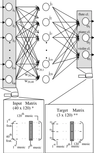
Artificial Neural Networks (ANN) [4] are computational models that try to emulate the behavior of the human brain. They are based on a set of simple processing elements, highly interconnected, and with a massive parallel structure. ANNs are characterized by their learning, adapting and generalization capabilities, which make them particularly suited for tasks such as function approximation.Feedforward Neural Networks (FFNN) are a special class of ANNs, in which all the nodes in some layer l are connected to all the nodes in layer l-1. Each neuron receives information from all the nodes in the previous layer and sends information to all the nodes in the following layer. A FFNN is composed of the input layer, which receives data from the exterior environment, typically one hidden layer (though more layers may be used [11]) and the output layer, which sends data to the exterior environment (Figure 1).
The links connecting each pair of neurons are given some weight, w. This attribution of weights to links is the job of any training algorithm, as described below. Each neuron computes an output value based on the input values received, the weights of the links from the neurons in the previous layer and the neuron’s activation function. Usually, sigmoid functions are used [4].
The capability of the FFNN for mapping input values into output values depends on the link weights. Their optimal determination is still an open problem. Therefore, iterative hill-climbing algorithms are used. Their main limitation comes from the fact that only local optima are obtained:
only occasionally the global optimum can be found. In the context of ANNs, these iterative optimization algorithms are called training algorithms.
Figure 1. FFNN used on the classification of music in three musical genres (flute, piano and violin). ANNs are usually trained in a supervised manner, i.e., the weights are adjusted based on training samples (input-output pairs) that guide the optimization procedure towards an optimum. For instance, in the case of our music genre classification, each network input is a vector with the 40 extracted features and each target value has a value of 1 for the correct class and a value of 0 otherwise (Figure 1). Our FFNN is trained in batch mode, i.e., all the training pares are presented to the network, an error measure is computed and only then the weights are adjusted towards error reduction. In Figure 1, we have a 40×120 input matrix where each line corresponds to a
particular feature and each column corresponds to each music feature-vector used for training the network. In the same figure, a 3×120 target output matrix is presented, where each column has information regarding the target class for the corresponding music feature-vector: all the lines have zero value, except for the line corresponding to the correct class, which has a value of one. For example, if the Tth music signature denotes a piano piece, and the second output neuron was assigned to the piano category, then the Tth ouput column would have a value of 1 in the second line, and zero for all other lines.
The most widely used training algorithm for FFNNs is backpropagation [4]. Here, there is a forward pass where inputs are presented to the network and output values are computed. The error between each target value and the corresponding output value is then calculated. Then, a backward pass is performed, where the weights are adjusted towards error reduction, using the gradient descent method. This process is repeated iteratively until the error is below a given threshold.
The gradient descent method has some limitations regarding convergence properties: the algorithm can get stuck in a local minimum and the selection of the learning rate is usually not trivial (if its value is too low, learning is slow; if it is too high, the network may diverge). Therefore, some variants are used, e.g., learning with a momentum coefficient or defining an adaptive learning rate [4].
Here, we use the Levenberg-Marquardt algorithm, which has the advantage of being significantly faster (10 to 100 times faster [1]) at the cost of higher memory consumption, due to the computation of a Jacobian matrix in each iteration. Also, this algorithm converges in situations where others do not [3].
After training, the neural network must be validated, i.e., its response to unknown data must be analyzed in order to evaluate its generalization capabilities. Thus, a forward pass is performed, with samples never presented before, and the same error measure used during training is computed. Typically, the available samples are divided in two sets, one for training and the other for validation, 2/3 for the former and 1/3 for the latter, respectively.
In order to avoid numerical problems, all the features were previously normalized to the [0, 1] interval [1].
4. Experimental Results
As stated before, our goal is to classify classical music into five subgenres: flute, piano, violin, choral and opera. These can be organized in a hierarchical manner, as depicted in Figure 2. The presented taxonomy is defined
.
.
.
.
.
.
i1 i2 i3 i39 i40 j2 j3 j20 j19 w20,40 w20,39 w20,1 j1 o1 o2 o3 flute cl. piano cl. violin cl. Input Matrix (40 x 120) * Tth music 1st music 1st feat. 40th feat. 120th music .. .. .. .. .. .. . . . . . . . . . . . . . . . . . Target Matrix (3 x 120) ** Tth music 1stmusic o1 120th music .. .. .. .. .. .. . . . . . . . . o2 o3 .. . . .. .. . .only for the sake of clarity: the practical classification performed was not hierarchical.
We collected a database of 300 monaural musical pieces (60 for each genre), sampled at 22050 Hz, with 16 bits quantization. For each piece, 6 seconds’ segments were extracted, based on their relevance for the genre in cause, as stated in Section 2.
Figure 2. Classical music genre classification. Our first goal was to discriminate between three genres of instrumental music: music for flute, piano and violin. The 6s’ segments extracted were chosen so as to include soles from each instrument by single or several players in unison, in isolation (monophonic segment) or with an orchestra in the background (polyphonic segment). For example, in the case of violin, we extracted a segment from “Spring” in Vivaldi’s Four Seasons.
In our second goal, we wanted to discriminate between genres of vocal music: chorals and opera. Typically, the musical pieces used for opera were vocal soles, essentially performed by tenors, sopranos and mezzo-sopranos (Callas, Pavarotti, etc.), whereas for choral music segments of simultaneous distinct voices were used without many of the stylistic effects used in opera (vibrato, tremolo). Many of the used pieces were also a cappela, i.e., only human voices, no instruments.
Finally, our third goal was to discriminate between all of the five genres referred above.
For the three problems addressed we used three-layered FFNNs, trained in batch mode via the Levenberg-Marquardt algorithm. Each network consists of 40 input neurons (one for each extracted feature) a variable number of hidden neurons (described below) and 2, 3 or 5 output neurons, according to problem under analysis. Both hidden and output neurons use sigmoid activation functions. For training purposes, we used 40 pieces from each genre, whereas for validation the remaining 20 were used (a total of 200 pieces for training and 100 for validation). Special care was taken so that the training samples for each genre were diverse enough.
Validation, i.e., classification of unknown pieces, was carried out under two different perspectives that we designate as percentage calculus rule 1 (PCR1) and percentage calculus rule 2 (PCR2).
PCR1
Under this perspective, a musical piece from a particular genre is well classified when the highest network output corresponds to that genre and its value is above or equal 0.7 (recall that the network outputs values between 0 and 1). In this situation, the piece considered is correctly classified, without any ambiguities.
When all output values are under 0.7, it is concluded that this particular musical piece does not belong to any of the defined categories. The highest value is not high enough to avoid possible ambiguities.
In order to improve class distinguishability, we check, for each well-classified piece, if the second highest network output value is at least 0.2 below the highest one. For this purpose we define the “gn2 < 0.2” measure, which represents the percentage of pieces where the second highest value was less than 0.2 below the highest one. For instance, if a musical piece has a value of 0.8 for the right genre (highest value) and 0.65 for the second highest value, this particular piece will make part on the “gn2 < 0.2” measure. In this situation, it is concluded that this piece shows some ambiguity regarding those genres.
PCR2
In this case, a musical piece from a particular genre is well classified if the highest network output value corresponds to the right genre, regardless of its amplitude.
We further define the “gn2 > 0.7” measure, which represents the percentage of wrongly classified pieces, where the correct genre corresponds to the second highest value, which is at least 0.7. The idea is to check if the piece is “almost” correctly classified.
Below we present the results for each of the classification problems addressed.
4.1. First Classification: Three Genres
In this case, musical pieces were classified into flute, piano and violin pieces.
For the determination of the most adequate number of neurons in the hidden layer, we tested several values in the range [10, 30]. The best classification results were obtained for 20 neurons in the hidden layer: an average classification accuracy of 83,3% for PCR1 and 85% for PCR2, for the three genres.
Regarding PCR1 analysis (Table 1), we got 85% accuracy for flute, 80% for piano and 85% for violin. Analyzing the results for flute pieces, we also notice that classical music
flute choral piano violin opera
vocal instrumental
5% of them were wrongly classified as piano, 5% as violin and 5% did not belong to any of the classes. We also see that the distance between the correct value and the second highest value was always at least 0.2 (“gn2 < 0.2” = 0%).
PCR1 83,3%
flute Piano Violin
Flute 85 10 5
Piano 5 80 10
Violin 5 10 85
unclassif. 5 0 0
gn 2 < 0.2 0 0 0
Table 1. Instrumental music confusion matrix: PCR1. As for PCR2 analysis (Table 2), we got 90% accuracy for flute, 80% for piano and 85% for violin. For violin pieces, 10% of pieces were wrongly classified but the violin class was the second highest value, which was above 0.7 (“gn2 > 0.7” = 10%).
PCR2 85% flute piano violin
Flute 90 10 5
Piano 5 80 10
Violin 5 10 85
gn 2 > 0.7 0 0 10
Table 2. Instrumental music confusion matrix: PCR2. By inspection of the classification errors, we noticed that they occur when the instruments are played in an unusual manner, not included in the training samples. For instance, two violin pieces were classified as piano, which had in common the fact of being extremely slow and having small amplitude variations. However, the output values for the violin class were high (above 0.7), which comes from the fact that the timbral features correctly detected the presence of violins.
4.2. Second Classification: Three Genres
In this situation, musical pieces were classified into opera and choral pieces. We obtained best classification results with 25 neurons in the hidden layer: an average classification accuracy of 90%, both for PCR1 and PCR2, for the two genres used.Regarding PCR1 analysis (Table 3), we obtained 90% accuracy for choral pieces and also 90% for opera.
PCR1 90% choral opera
choral 90 10
opera 10 90
unclassif. 0 0
gn 2 < 0.2 0 0
Table 3. Vocal music confusion matrix: PCR1. As for PCR2 analysis (Table 4), we obtained the same results: 90% accuracy both for opera and choral pieces.
PCR2 90% choral opera
choral 90 10
opera 10 90
gn 2 > 0.7 0 0
Table 4. Vocal music confusion matrix: PCR2. Only two choral pieces and two opera pieces were not correctly classified. One of those choral pieces has some instrumental parts, unlike most of the training samples, which are a capella. Also, that particular piece has a female voice that clearly stands out, which the average human being could easily classify as opera. As for the two mistaken opera pieces, we could not find any clear reasons for that behavior. The only conclusion we can draw is that the used features are good enough for the well-behaved cases. For more atypical situations, a more thorough feature analysis is required: elimination of redundant features and/or inclusion of necessary extra features.
4.3. Third Classification: Five Genres
Here, musical pieces were classified into the five categories listed before: flute, piano, violin, opera and choral music. Best classification results were obtained with 20 neurons in the hidden layer for PCR1, with 64% average classification accuracy, and 30 neurons for PCR2, with 76% average classification accuracy, for the five genres used.
Regarding PCR1 analysis (Table 5), we obtained 65% classification accuracy for flute pieces, 65% for piano, 70% for violin, 50% for chorals and 70% for opera. PCR1 64% flute piano violin choral opera
Flute 65 15 5 0 10 Piano 10 65 0 10 0 Violin 0 10 70 10 0 Choral 15 0 5 50 0 Opera 0 0 5 15 70 unclassif. 10 10 15 15 20 gn 2 < 0.2 0 10 20 5 15
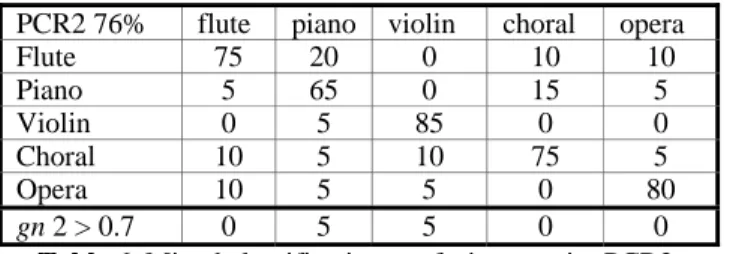
Table 5. Mixed classification confusion matrix: PCR1. As for PCR2 analysis (Table 6), the classification accuracy was 75% for flute pieces, 65% for piano, 85% for piano, 75% for chorals and 80% for opera.
PCR2 76% flute piano violin choral opera Flute 75 20 0 10 10 Piano 5 65 0 15 5 Violin 0 5 85 0 0 Choral 10 5 10 75 5 Opera 10 5 5 0 80 gn 2 > 0.7 0 5 5 0 0
Table 6. Mixed classification confusion matrix: PCR2. Though interesting, the results obtained for this more complex classification problem are less satisfactory. It is clear that the used features could not separate the five classes in a totally unambiguous manner. Therefore, a deeper feature analysis seems fundamental in order to obtain better results.
5. Conclusions
The main goal of this paper was to present a methodology for the classification of classical music. Although the results obtained are not sufficient for real-world applications, they are promising.
In the most complex case, where we defined five categories, the classification results were less accurate. However, in our opinion a hierarchical classifier, following the structure in Figure 3, would lead to better results.
In the future, we will conduct a more thorough analysis of the feature space: detection and elimination of redundant features, as well as definition and utilization of other features, which may help to discriminate the more atypical cases. Additionally, we plan to use a broader and deeper set of categories, i.e., more basis classes and subclasses. In case we use categories like waltz, rhythmic features, not used in the present work, will certainly be important.
Acknowledgments
This work was partially supported by the Portuguese Ministry of Science and Technology (MCT), under the program PRAXIS XXI.
References
[1] Demuth, H., Beale, M., “Neural Network Toolbox User’s Guide”, version 4, Mathworks, 2001
[2] Golub, S., “Classifying Recorded Music”, MSc Thesis, University of Edinburgh, 2000
[3] Hagan, M., Menhaj, M., “Training Feedforward Networks with the Marquardt Algorithm”, IEEE Transactions on Neural Networks, vol. 5, no. 6, November 1994
[4] Haykin S., “Neural Networks: A Comprehensive Foundation”, Macmillan College Publishing, 1994 [5] Kosina, K., “Music Genre Recognition”, MSc
Thesis, Hagenberg, 2002
[6] Lu, L., Jiang, H. and Zhang, H., “A Robust Audio Classification and Segmentation Method”, ACM MM 2001
[7] Martin, K., “Toward Automatic Sound Source Recognition: Identifying Musical Instruments” NATO Computational Hearing Advanced Study Institute, Il Ciocco, Italy, 1998
[8] Martin, K. D., Scheirer, E. D., Vercoe, B. L., “Musical content analysis through models of audition”, ACM Multimedia Workshop on Content-Based Processing of Music, 1998
[9] Perrot, D., and Gjerdigen, R.O., “Scanning the dial: An exploration of factors in the identification of musical style”, Proceedings of the 1999 Society for Music Perception and Cognition
[10] Polikar, R., “The Wavelet Tutorial”, http://engineering.rowan.edu/~polikar/WAVELETS/ WTtutorial.html, available by July 2003
[11] Sarle W. (maintainer), “Neural Nets FAQ”, ftp://ftp.sas.com/pub/neural/ FAQ3.html, 2001 [12] Smith, S., “The Scientist and Engineer's Guide to
Digital Signal Processing”
[13] Tzanetakis, G. and Cook, P., “Musical Genre Classification of Audio Signals”, IEEE Transactions on Speech and Audio Processing, vol. 10, no. 5, July 2002
[14] Tzanetakis, G., Essl, G. and Cook, P., “Automatic Musical Genre Classification of Audio Signals”, ISMIR 2001