Improving Load Balancing in Virtualized
Environments using Pearson’s Correlation
Sorocaba, SP
Improving Load Balancing in Virtualized
Environments using Pearson’s Correlation
Dissertação de mestrado apresentada ao Pro-grama de Pós-Graduação em Ciência da Com-putação (PPGCC-So) da Universidade Fed-eral de São Carlos como parte dos requisi-tos exigidos para a obtenção do título de Mestre em Ciência da Computação. Linha de pesquisa: Engenharia de Software e Sis-temas de Computação.
Universidade Federal de São Carlos – UFSCar
Centro de Ciências em Gestão e Tecnologia – CCGT
Programa de Pós-Graduação em Ciência da Computação – PPGCC-So
Supervisor: Prof. Dr. Fábio Luciano Verdi
Moraes Filho, Nilson Rubens de
Improving Load Balancing in Virtualized Environments Using Pearson's Correlation / Nilson Rubens de Moraes Filho. -- 2018.
108 f. : 30 cm.
Dissertação (mestrado)-Universidade Federal de São Carlos, campus Sorocaba, Sorocaba
Orientador: Fábio Luciano Verdi
Banca examinadora: Mateus Augusto Silva Santos, Gustavo Maciel Dias Vieira
Bibliografia
1. Load Balancing. 2. Virtualization. 3. Pearson Correlation. I. Orientador. II. Universidade Federal de São Carlos. III. Título.
Ficha catalográfica elaborada pelo Programa de Geração Automática da Secretaria Geral de Informática (SIn).
DADOS FORNECIDOS PELO(A) AUTOR(A)
I would like to acknowledge and thank,
God, as the source of all inspiration. "For the Lord gives wisdom, from his mouth come knowledge and understanding" (Prv 2, 6).
My parents, that always believed in my potential and encourage me to keep moving forward.
My wife, that supported me during this long journey and understood all the time and effort that it took me to get here, helping me to surpass all difficulties.
My kids, that had patience during all the countless weekends that I had to study.
To my family, in special my sisters, that were always on my side.
The companies Convergys and Qlik, for allowing me to pursue this dream.
My director Cesar Ripari and manager Alexandre Zacarias for supporting me at work during the conclusion of this dissertation.
Prof. Fábio, for all the knowledge transfer, helpful insights, persistence and support to assist me getting this project done.
All UFSCAR PPGCCS teachers, for the excellent classes and dedication.
All UFSCAR employees, especially Roberto Romualdo Marvulle, that supported us during the whole course.
My colleagues from the LERIS laboratory, especially André Beltrami.
UFSCAR, to seek and provide high quality education for its students.
Virtualização é um dos alicerces da computação em nuvem pois permite melhor utilização de recursos computacionais em um centro de dados. Existem diferentes abordagens para virtualização que oferecem a mesma funcionalidade, mas com diferentes níveis de abstração e métodos. Neste sentido podemos citar o uso de Máquinas Virtuais e contêineres. Definimos Elemento Virtual (EV) como sendo uma máquina virtual ou contêiner, e usaremos este conceito para generalizar a nossa proposta de balanceamento de carga. O balanceamento de carga pode ser realizado através da migração dos EVs, reduzindo o consumo de energia, disponibilizando uma melhor distribuição dos recursos computacionais e permitindo que clientes movam EVs de um provedor de nuvem para outro que ofereça melhor SLA ou custo. Existem alguns métodos que tratam da melhora do balanceamento de carga em um centro de dados. Um deles utiliza o coeficiente de correlação de Pearson relacionado ao consumo de CPU, para migrar EVs de um servidor sobrecarregado para outro que possua melhor disponibilidade de recursos. O coeficiente de correlação de Pearson estima o grau de dependência entre duas quantidades. Já a migração em tempo real é uma característica da virtualização que permite que um EV seja transferido de um servidor para outro, mantendo a execução dos processos ativos. Porém migrar um EV que possua forte dependência em relação ao tráfego de rede interno do servidor, pode gerar um aumento do consumo de recursos computacionais do ambiente. Isto devido ao aumento do consumo de rede ocasionado pela migração do EV para outro servidor que, topologicamente, esteja distante do servidor atual. Esta dissertação tem como objetivo definir uma heurística para melhorar o processo de decisão de migração de EVs. A heurística utiliza o coeficiente de correlação de Pearson e leva em conta não só o consumo de CPU mas também o tráfego de rede interno entre EVs. Os resultados mostraram que o uso da heurística, em um ambiente com tráfego de rede interno entre EVs, melhorou o processo de decisão em 18%, comparado com o método que considera apenas o coeficiente de correlação baseado em CPU.
Palavras-chaves: Virtualização. Máquina Virtual. Contêiner. Correlação de Pearson.
Virtualization is one of the foundations of cloud computing as it allows better utilization of computing resources in a data center. There are different virtualization approaches that offer similar functionality, but with different levels of abstraction and methods. In this sense we can mention the use of Virtual Machines and containers. We define Virtual Element (VE) as a virtual machine or a container, and we will use this concept to make our load balancing approach generic. Load balancing can be achieved through live migration of VEs, reducing energy consumption, enabling better distribution of computational resources and allowing customers to move VEs from a cloud provider to another one that may offer better SLA or costs. There are some methods that addresses the load balancing improvement in a data center. One of them applies the Pearson correlation coefficient related to CPU usage, to migrate VEs from an overloaded host to another that have better availability of resources. The Pearson correlation coefficient estimates the dependency level between quantities. Yet, live migration is a virtualization feature that allows a VE to be transferred from one equipment to another, keeping the active processes running. However, to migrate a VE that has strong dependency with the internal network traffic from a host, can create an increase in the overall network consumption due to the migration of the VE to another server, topologically distant from the current host. This dissertation defines a heuristic that has as objective improve the migration decision process of VEs. The heuristic applies Pearson’s correlation coefficient and takes in consideration not only CPU consumption, but also the internal network traffic between VEs. Results shown that the application of the heuristic improved the decision process in at least 18% compared to a method that considers only CPU correlation coefficient.
Key-words: Virtualization. Virtual Machine. Container. Pearson Correlation. Live
Figure 1 – Service models in a cloud environment. . . 26
Figure 2 – Container as a Service (CaaS).. . . 26
Figure 3 – Decision process example. . . 28
Figure 4 – VM Migration Phases. . . 39
Figure 5 – Container Migration Phases. . . 39
Figure 6 – Container Migration Pre-Copy Memory. . . 40
Figure 7 – Container Migration Post-Copy Memory. . . 40
Figure 8 – Heuristic hT X . . . 48
Figure 9 – Decision/Monitoring Scenario. . . 51
Figure 10 – Decision/Monitoring Instantiation. . . 52
Figure 11 – Decision/Monitor Flowchart.. . . 53
Figure 12 – Monitor Module - Docker Implementation. . . 59
Figure 13 – Container Migration Phases . . . 63
Figure 14 – Container Image and Layers.. . . 64
Figure 15 – Number of hosts and containers. . . 68
Figure 16 – Container allocation. . . 68
Figure 17 – Container Migration Results - 1000 Hosts. . . 70
Figure 18 – CPU Mean. . . 71
Figure 19 – CPU standard deviation. . . 71
Figure 20 – CPU variance between ¯x−1σ and ¯x+ 1σ (a). . . 72
Figure 21 – CPU variance between ¯x−1σ and ¯x+ 1σ (b). . . 72
Figure 22 – Number of hosts with CPU above 70%. . . 73
Figure 23 – Percentage Reduction in the number of overloaded hosts. . . 74
Figure 24 – Number of migrations and % Reduction. . . 74
Figure 25 – Migration Comparison between heuristic and high correlated hosts. . . 75
Figure 26 – Testbed Environment. . . 76
Figure 27 – Stress CPU Example. . . 77
Figure 28 – Iperf external traffic. . . 80
Figure 29 – Iperf internal traffic. . . 81
Figure 30 – Container Migration Results - 100 Hosts . . . 100
Figure 31 – Container Migration Results - 300 Hosts . . . 101
Figure 32 – Container Migration Results - 500 Hosts . . . 102
Figure 33 – Container Migration Results - 1000 Hosts . . . 103
Figure 34 – Container Migration Results - 2500 Hosts . . . 104
Table 1 – Pearson correlation coefficient score levels . . . 44
Table 2 – Definitions . . . 45
Table 3 – Heuristic scores for hT X . . . 47
Table 4 – test Definitions . . . 73
Table 5 – Number of migrations comparison between Heuristic and CPU only method 74 Table 6 – Migration Comparison between heuristic and high correlated hosts. . . . 75
Table 7 – Initial State - CPU percentage load . . . 107
Table 8 – Results after Pearson correlation considering CPU only method . . . 107
Table 9 – Results After Heuristic . . . 107
API Application Programming Interface
CaaS Container as a Service
CoW Copy-on-write
CRIU Checkpoint Restore In Userspace
GB Gigabytes
HA High Availability
HPC High Performance Computing
IaaS Infrastructure as a Service
I/O Input/Output
JSON JavaScript Object Notation
KB Kilobytes
MB Megabytes
OS Operating System
PaaS Platform as a Service
REST Representational State Transfer
RX Received Data
SaaS Software as a Service
SLA Service Level Agreement
TX Transmitted Data
VE Virtual Element
1 INTRODUCTION . . . 25
2 RELATED WORKS . . . 31
2.1 Basic Concepts . . . 31
2.2 Related Works . . . 34
3 PEARSON CORRELATION MODEL . . . 43
3.1 Pearson Correlation Coefficient. . . 43
3.2 Proposed Heuristic Model. . . 45
3.3 Heuristic based on CPU . . . 49
4 ARCHITECTURE AND IMPLEMENTATION . . . 51
4.1 Decision/Monitoring Architecture . . . 51
4.2 Implementation . . . 58
5 TESTS AND RESULTS . . . 67
5.1 Simulation . . . 67
5.2 Testbed . . . 76
5.2.1 Stress command . . . 77
5.2.2 Iperf command - External Data Traffic . . . 80
5.2.3 Iperf command - Internal Data Traffic . . . 81
Conclusion . . . 83
Bibliography . . . 85
APPENDIX A – COMMAND OUTPUTS . . . 89
A.1 Docker API JSON Response - call GET . . . 89
A.2 Docker API JSON Response - container statistical data . . . 91
A.3 Decision Module Output - CPU Stress Test . . . 94
A.4 Monitor Migration Module - Sub-Module Migrate Output - CPU Stress Test . . . 94
A.5 Monitor Migration Module - Sub-Module Restore Output - CPU Stress Test . . . 95
A.6 Monitor Module Output - CPU Stress Test . . . 95
A.7 Decision Module Output - External IPERF Test . . . 96
A.9 Monitor Module Output - Internal IPERF Test . . . 97
A.10 Decision Module Output - Internal IPERF Test . . . 97
A.11 IPERF Server and Client Output - Internal IPERF Test . . . 98
APPENDIX B – CONTAINER MIGRATION PERFORMANCE . . 99
B.1 100 Hosts Simulation Results. . . 100
B.2 200 Hosts Simulation Results. . . 101
B.3 500 Hosts Simulation Results. . . 102
B.4 1000 Hosts Simulation Results . . . 103
B.5 2500 Hosts Simulation Results . . . 104
B.6 5000 Hosts Simulation Results . . . 105
APPENDIX C – SUPPORTING TABLES . . . 107
C.1 Initial State - CPU Table Statistics . . . 107
C.2 After applying hCPU - CPU Table Statistics . . . 107
C.3 After applying hTot - CPU Table Statistics. . . 107
1 Introduction
Data center is a facility responsible for handling servers, mainframes, data storage and networking. The name data center comes from the fact that, in a centralized envi-ronment, all the devices are physically located in the same place. Cloud computing is an extension of this paradigm, in which a series of virtualized resources, like hardware and development platforms, can be exposed as services and be accessed through the network (BUYYA et al., 2009). These resources can be dynamically reconfigured and adjusted to different loads, allowing an optimized allocation of resources, concept called elasticity. Resources are typically explored in a pay per use model in which the infrastructure provider guarantee a certain level of service defined in a service level agreement (SLA)(VAQUERO et al., 2008). Companies can reduce their operational costs using the same services in the cloud, instead of providing them on premises (BUYYA et al., 2009). Providers like Amazon, Google, Microsoft, IBM, among others, have established data centers around the world in order to provide cloud services.
Virtualization is one of the cloud computing pillars, allowing providers to maximize their hardware processing power, offering elasticity and scalability of resources. There are different virtualization approaches that offer similar functionality, but with different levels of abstraction and methods. Virtual Machines (VMs) are one of the most used methods. VMs work with hardware emulation through a component called hypervisor, that offers isolation and it is responsible to execute different kernels or operating systems (OSs) under the same physical hardware. Example of solutions that work with hypervisors are VMWare (VMWARE, 2018), KVM (KVM, 2018), Xen (XEN, 2018) and Microsoft Hyper-V (HYPER-V, 2018). Nevertheless, in order to provide security and isolation of process and applications, this type of virtualization has a high performance impact.
Another method, in which computational resources are allocated more efficiently, is called virtualization by containers (JOY, 2015). Containers are a lightweight version of the OS, not having the VMs overload. Containers do not emulate I/O and offer isolation, portability, reduced initialization time and better performance compared to VMs (LI; KANSO, 2015). In order to provide isolation, containers use Linux OS functionalities like namespaces, control groups and chroot (LI; KANSO; GHERBI, 2015)(FELTER et al.,
2015). As examples of container solutions we can mention OpenVZ (OPENVZ, 2018), LXC (LXC, 2018), Rkt (RKT, 2018) and Docker (DOCKER, 2018). The last is a good example of container platform that has been widely used in the market (RIGHTSCALE,
26 Chapter 1. Introduction
With the adoption of containers in the data center, a new type of service model, called CaaS (Containers as a Service) has appeared (PIRAGHAJ et al.,2015). This service complements the existing IaaS (Infrastructure as a Service), PaaS (Platform as a Service) and SaaS (Software as a Service)(MELL; GRANCE et al., 2011) service models. Figure 1
details how the cloud service models have evolved over time:
Figure 1: Service models in a cloud environment.
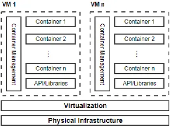
PaaS makes extensive use of VMs, although virtualization by VMs imposes an overhead regarding resource consumption for applications that demand elasticity (LI; KANSO; GHERBI,2015). Figure 2 details the new CaaS service model, in which we have containers running inside VMs. This model has been adopted in data centers as offers VMs security and containers scalability.
Figure 2: Container as a Service (CaaS).
running (ELSAID; MEINEL, 2014)(CELESTI et al., 2010)(ASHINO; NAKAE,2012). VM migration involves the transfer of larger files, making the VM migration process costly, from the network consumption perspective and platform down time. As container images are smaller, the migration process does not have the same cost.
VM and container migration can be used to better distribute the load depending on CPU utilization and network traffic. Migration and load balancing are also important in order to consolidate running applications in less servers during periods of low utilization (green computing)(KANSAL; CHANA,2012). Another motivation is to allow enterprises to freely choose the best cloud provider depending on a series of factors, like cost, availability or better SLAs. In this scenario, enterprises could choose to live migrate VMs or containers from one cloud provider to another (hybrid cloud) (LINTHICUM,2016).
Let us define host as any physical server in a data center environment and Virtual Element (VE) as any virtual machine or container. The VE concept will be used in this document to make our approach generic.
Problem and Objective
One of the problems for data centers and cloud providers is to better distribute the work load between available hosts. A better distribution will reduce power consumption and provide better allocation of available resources. The objective of this dissertation is to present a heuristic that improves the live migration decision process of VEs taking into consideration not only CPU usage, but also network data traffic.
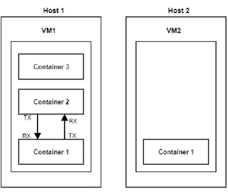
Figure 3 will help clarifying the problem and the objective of this work. Let us suppose that we have two hosts in one rack. Each host has one VM running, defined here as VM1 and VM2 respectively. VM2 has one container running that consumes very low CPU. Therefore, host 2 is under-loaded. VM1 is running 3 containers. Container 1 and container 2 have network traffic between each other. Suppose that host 1 becomes overloaded as its CPU goes above a specified threshold. The problem here is to decide which of the 3 containers should be migrated to host 2 in order to improve load balancing. One of the existing migration models uses Pearson correlation coefficient (PEARSON,
1895) monitoring only CPU consumption to make a decision (PIRAGHAJ et al., 2015). Consider that container 2 is the one that is consuming more CPU at host 1. Based on this model, container 2 should be migrated. However, if we migrate container 2 to host 2, we will improve load balancing, but, additional traffic in the network will be generated. Our proposed approach is to apply a heuristic that takes also in consideration network traffic in the decision process, using Pearson correlation coefficient as well. It is important to take into consideration network traffic, as tests have shown that power consumption raises with the increase in network traffic (MORABITO, 2015).
28 Chapter 1. Introduction
Figure 3: Decision process example.
host. If we migrate a VE that has network activity inside the same host, we may improve overall CPU utilization, but we will increase network traffic between hosts. An architecture was implemented to validate the assertiveness of the heuristic. It is not the intent of this dissertation to discuss how live migration of VEs is implemented for the different solutions available. Our focus is on the decision process itself.
The contributions of this dissertation to the scientific community are:
• Apply the Pearson correlation coefficient (PEARSON, 1895) with CPU and network
traffic during the migration decision process. Piraghaj et al. (PIRAGHAJ et al.,2015) monitored only at CPU consumption. We extend this concept looking at network traffic as well;
• Perform live migration of VEs that have low correlation coefficient for internal
network traffic and high correlation for CPU usage. Main objective is to better distribute the work load at the data center taking in consideration both CPU and network traffic;
• Define a heuristic as foundation to the decision migration process. The heuristic
score depends on the Pearson correlation coefficient for CPU and network traffic. Depending on the calculated score, the decision of migrating the VE is taken or not.
The remaining of this dissertation is organized as follows:
• Chapter 2: it presents the theoretical foundation and related works that are the basis
for this project;
• Chapter 3: it describes the Pearson correlation coefficient and how it relates with
this project. Furthermore, a heuristic is defined and its application is described in the decision process;
• Chapter 4: it details the architecture developed to validate the heuristic and all its
elements. A description of the implementation is explained;
• Chapter 5: it describes the test methodology and its respective results;
• Conclusion: it contains our final remarks and future works that can be developed
2 Related Works
This chapter describes the works that are related to this project. The first Section provides basic concepts that are important for the understanding of the scope of the dissertation. The following Section details work that is relevant and that served as motivation to the development of the presented solution.
2.1 Basic Concepts
This Section describes basic concepts of the cloud environment and the available cloud service models, like IaaS, PaaS, SaaS and CaaS. The VM and container virtualization approach are defined here and how these technologies have been used in data centers. Live migration is a fundamental characteristic that will be discussed as well. The next Section will expand the concepts presented here.
Buyya et al. (BUYYA et al.,2009) defines cloud computing as:
A type of parallel and distributed system consisting of a collection of inter-connected and virtualized computers that are dynamically provisioned and presented as one or more unified computer resource(s) based on service level agreements established through negotiation between the service provider and consumers.
Enterprises are interested in the cloud model as it represent a cost reduction com-pared to the on-premises model, in which companies need to invest in all the infrastructure. Buyya et al. (BUYYA et al., 2009) show how infrastructure based on virtualization of resources is utilized to offer scalability and elasticity.
The National Institute of Standards and Technology (NIST) (MELL; GRANCE et al., 2011) define five essential characteristics for the cloud model:
• On-demand self-service: consumer can provision computing resources as needed;
• Broad network access: capabilities are available over the network;
• Resource pooling: computing resources are pooled to serve multiple consumers
using a multi-tenant model, with different physical or virtual resources allocated on demand. There is a sense of location independence, i.e, the customer has no control or knowledge over the exact location of the provided resources;
• Rapid elasticity: capabilities can be elastically provisioned and released, in some cases
32 Chapter 2. Related Works
• Measured service: resource usage can be monitored, controlled and reported, providing
transparency for the cloud provider and to the consumer.
Vaquero et al. (VAQUERO et al., 2008) associated cloud to a new way to provide computing infrastructure. Cloud paradigm shifts infrastructure to the network in order to reduce management costs with hardware and software. The authors defined cloud as a large pool of usable and accessible virtualized resources that can be dynamically adjusted to a variable load. Resources are charged in a pay-per-use model that guarantees an agreed SLA. IaaS is defined as a large set of computing resources, like storage and processing capacity, that, through virtualization, can be dynamically offered to companies to run their services. PaaS is an additional abstraction level in which the platform is offered to run customer services. Yet, SaaS is an alternative to run applications, using services that are hosted in the cloud.
According to the National Institute of Standards and Technology (NIST) (MELL; GRANCE et al., 2011) the service models in a cloud environment are:
• Software as a Service (SaaS): the capability offered to consumers to use provider’s
application, running on a cloud infrastructure. The consumer does not manage or control the underlying cloud infrastructure, with the exception of some application configuration;
• Platform as a Service (PaaS): the capability provided to the consumer to deploy onto
the cloud infrastructure consumer’s applications. The consumer does not manage or control the underlying cloud infrastructure, but has control over the deployed application;
• Infrastructure as a Service (IaaS): the capability provided to the consumer to
provision processing, storage, networks, and other computing resources where the consumer is able to deploy and run software, which can include OSs and applications. The consumer does not manage or control the underlying cloud infrastructure, but has control over OS, storage and deployed application.
NIST also defines the possible deployment models:
• Private Cloud: cloud infrastructure provisioned exclusively by a single organization to
• Public Cloud: cloud infrastructure provisioned for open use by general consumers.
It may be owned, managed and operated by a business, academy, government or a combination of them. It exists on the premises of the cloud provider;
• Hybrid Cloud: cloud infrastructure is a composition of two or more distinct cloud
infrastructures (private or public) that remain unique entities. There is a standardized or proprietary technology that enables data and application portability.
Clark et al. (CLARK et al.,2005) mentioned that a VM encapsulate access to a set of physical resources. Amaral et al. (AMARAL et al., 2015) defined virtualization as a technology that allows the data center to offer on-demand and elastic resources. VMs have been widely used in traditional data centers and cloud environments (private, public and hybrid clouds), nevertheless, the interest in container technology has increased as containers are lightweight and fast. Containers provide less overhead compared to VM because they do not emulate a full physical hardware virtualization. Containers use Linux cgroups and namespaces to provide isolation of processes and file systems. Containers biggest advantage is the capability to run a copy of the Linux OS without running a hypervisor. The authors also discussed a new trend called microservices. A system can be developed in small sets, called microservices, that can be developed, managed and scaled independently. As microservices are a small set of the whole system, they fit very well with the concept of the lightweight containers.
Live migration is a powerful feature in a virtualized data center that can be used for load balancing, reduce power consumption, disaster recovery, among others. Elsaid & Meinel (ELSAID; MEINEL, 2014) studied the VM live migration impact considering network resources and power consumption.
Regarding performance, Felter et al. (FELTER et al.,2015) developed a comparison between VMs and containers. Their final results showed that containers have an equal or better performance in almost all proposed scenarios. The authors also detailed how containers implement isolation.
As far as the Pearson correlation coefficient (PEARSON, 1895) is concerned, Filho & Júnior (FILHO; JÚNIOR, 2009) described that the origin of this coefficient came from the research of Karl Pearson and Francis Galton (STANTON, 2001). According to the authors, Pearson correlation coefficient r is a measure of the linear association between
34 Chapter 2. Related Works
2.2 Related Works
There are several studies regarding the use of VMs in a cloud environment. The interest in containers has increased due to the benefits provided by this architecture. The combination of VMs and containers, concept called as CaaS, is a trend as it provides VM security and containers performance (RIGHTSCALE, 2016). Live migration of VMs and containers is an important feature for load balancing and high availability in a data center.
Bernstein (BERNSTEIN, 2014) mentioned that hypervisors and containers are part of the existing cloud environment. He details also the existence of a concept called bare metal cloud, in which the same characteristics of cloud technology are offered, but only in physical servers. The author observed that hypervisor based deployments are ideal when applications require different OSs on the same cloud. As containers share an OS, their deployment is much smaller in size compared to VMs, and its restart time, much quicker. Due to this characteristic, a container deployment can host hundreds of containers compared to VM deployments. Bernstein approached Docker (DOCKER,2018), an open source project, as a container technology that extends LXC containers (LXC, 2018) in order to provide faster Linux application development. Docker containers are created using base images. A base image can consist of just the OS or pre-built applications. The author commented about benchmarks that showed that containers are much faster than VMs, but also discussed that many deployments have decided for a hybrid implementation, with containers and VMs. One example of management solution that provides full VM and container integration is Proxmox VE (PROXMOX, 2018). Proxmox is a management platform with full integration with KVM hypervisor (KVM,2018) and LXC containers.
Microservices is a technology trend that has leverage the container architecture. A system can be developed in small sets called microservices that can be managed and scaled independently. Amaral et al. (AMARAL et al., 2015) analyzed performance of microservices in this environment. The cost of using microservices with containers is the computational overhead of running an application in different processes, and the increase in network traffic between containers. The increase in network traffic between containers is an issue that this work will address. Authors mentioned Kubernetes (KUBERNETES, 2018), an open source container cluster management solution developed by Google, that provides load balancing and failure management for containers. The objective of Kubernetes is to make the management of large number of microservices easier. Docker announced that has incorporated native support to Docker Swarm (DOCKERSWARM,2018) and Kubernetes in its platform. Docker Swarm is also a cluster management solution provided by Docker. Another container management system is called LXD (LXD, 2018). LXD is a layer on top of LXC that provides a REST API to manage containers and offers to the user the same experience as VMs. It is possible to run all flavors of containers inside LXD.
VMs and containers. Piraghaj & Buyya (PIRAGHAJ et al., 2015) developed a framework for container consolidation in a CaaS environment, in order to get a more energy efficient data center. The authors developed an algorithm that is invoked when the host CPU reaches a specific threshold. Then, they used the Pearson correlation coefficient (PEARSON,1895), based on CPU consumption, to decide if a container should be migrated or not. The article analyzed the correlation between host and container CPU. Our work take this concept as a reference, and adds network traffic at the live migration decision process. As the objective of the authors were to reduce power consumption in the data center, they used live migration to consolidate the work load in the smaller number of VMs as possible, and consequently, the smaller number of physical hosts. If there were hosts with no VMs and containers running after the migrations, the framework powered off these hosts. From the other side, if the framework detected that there were not enough VMs to run the processes, it invoked a module that creates more VM instances.
Still in the energy efficiency field, Morabito (MORABITO, 2015) compared power consumption of VM and containers. While both technologies present similar power con-sumption in idle state and also during CPU/memory stress test, during network tests VM showed a higher energy consumption compared to containers due to the fact that network packets need to be processed by extra layers in hypervisor environments. Network tests were done using iperf Linux tool (IPERF, 2018). The work developed by Morabito showed the importance of considering network traffic during load balancing in order to avoid unnecessary resource consumption.
Kansal & Chana (KANSAL; CHANA, 2012) described the importance that migra-tion, server consolidation and load balance have to green computing. The authors discussed existing load balancing techniques for cloud computing. They defined green computing as the implementation of policies and procedures that improve the efficiency of computing resources, reducing energy consumption and environmental impact.
36 Chapter 2. Related Works
evaluate how VMs communicate before deciding where to place them. For instance, if two VMs that communicate frequently are put in different physical servers, the CPU allocation criteria can be met, but can provide poor performance due to the frequent communication occurred between the VMs. They have developed a framework for VM placement that considers the software packages running on each VM. Based on the software packages, the framework make assumptions on how the VMs communicate, and decided where is the best place to run them.
Real time migration is an important feature available, not only in hypervisors, but also in containers, and can be used for load balancing, reduction in power consumption, disaster recovery, among others. Elsaid & Meinel (ELSAID; MEINEL, 2014) studied the overhead of VM live migration in the overall data center performance. Through live migration, a running VM is transferred from one physical server to another, with little interruption. Therefore, the study of resource consumption during VM live migration needs to be considered. The costs associated with live migration are: migration time and migration down time, overhead in power and CPU utilization and network bandwidth consumption. The authors described the VM live migration process using VMotion, a solution from VMWare (VMWARE, 2018), and created models to calculate the time to migrate and power consumption during the process. With those models, an estimation of live migration performance was done. Elsaid & Meinel have a concern regarding network bandwidth consumption, an issue that our work will address.
VM image size to be transferred during the migration is also a concern. Celesti et al. (CELESTI et al., 2010) explored the VM live migration process and described the concern of transferring GBs of data over the network. Authors focused on how to reduce the VM image size to be transferred during migration.
Ashino & Nakae (ASHINO; NAKAE,2012) analyzed VM migration to different hypervisor implementations. The authors reinforced the importance that VM migration is taken in cloud solutions, and that a VM migration method, between different hypervisor solutions, will be required. Current live migration process, when the destination is a different hypervisor, involves converting the VM image and the transfer of larger image files. VM image conversion can create boot problems at destination. The authors proposed a different migration method, that was destination dependent. With this approach, VM image was in general 20% smaller than the regular image.
having an orchestration tool to perform the live migration and monitor the whole process. Companies, like Jelastic (JELASTIC,2018), are implementing this type of orchestration tool.
As container adoption has increased, discussions about high availability (HA) and, consequently, real time migration has appeared. Romero & Hacker (ROMERO; HACKER,
2011) were one of the precursors in the study of container real time migration for parallel applications, especially with OpenVZ (OPENVZ, 2018). The authors decided to work with containers, compared to VMs, due to its lightweight characteristics. With containers, the amount of data to be dumped, moved and restarted is much smaller than compared to VMs. This characteristic will make the process quicker, what is very important when we talk about parallel applications.
Li & Kanso (LI; KANSO, 2015) compare VM and containers for achieving HA. One important aspect that the authors approached is a comparison between stateless and statefull containers. The first can have their state replicated in a storage and be deployed behind load balancers. Failures are transparent, as the load balancer will send traffic to healthy containers. Nevertheless, for statefull containers, in which the state of the application and the network stack needs to be maintained, the live migration approach is a viable alternative. VM and containers live migration is implemented through the checkpoint/restore capability. CPU compatibility is also required to ensure that a VM can perform normally at destination host after migration. OpenVZ (OPENVZ,2018) container technology was one of the first to implement the chekckpoint/restore functionality, however it was implemented as loadable modules in the OpenVZ kernel. The lack of integration with native Linux kernel reduced the adoption of OpenVZ. To solve this situation, CRIU (CRIU,2018) project was created, moving most of the checkpoint capability outside the kernel, into user space. With CRIU, one can freeze a running application and save it as a set of files in disk. Later these files can be used to restore the application and start it exactly from the point where it was frozen. Docker has adopted CRIU as a solution for checkpoint/restore. Currently this functionality is only available in Docker in experimental mode. Later it will available for production environments. Still in the HA topic, Kanso has developed another work with Gherbi (KANSO; HUANG; GHERBI, 2016), discussing the use of Kubernetes to manage containarized applications across multiple hosts. The authors mentioned that containers have been adopted to accelerate the development and operation of microservices, as microservices, in general, are loosely coupled and have independent life cycles and deployments. They have tested the effectiveness of Kubernetes (KUBERNETES,2018) to manage HA. Containers are grouped in what is called a pod.
38 Chapter 2. Related Works
The comparison between containers and VMs is also done by Xavier et al. (XAVIER et al.,2013) in a High Performance Computing (HPC) environment. The authors mentioned that the use of virtualization in HPC was avoided due to the performance overhead. However, with the enhancements on container virtualization, solutions like LXC (LXC,
2018) and OpenVZ (OPENVZ,2018) have been adopted in HPC environments. Techniques like live migration, checkpoint and resume are important in such environments.
Celesti et al. (CELESTI et al., 2010) defined cloud federation as an environment in which VMs can be migrated from a cloud to another. Their objective is to improve VM migration in such environment. VM migration implies the transfer of the VM image, causing consumption of network bandwidth and cloud resources. They proposed a mechanism that reduced the amount of data to be transferred. Each VM has a disk image, in a given hypervisor format, containing the file system and guest OS. There are two types of VM migration: hot (live) and cold. The biggest difference is that in hot migration the VM does not loose its status, and users does not notice any change, while in cold, users notice a service interruption. Downtime is defined as the time difference when a VM is turned it off in the source, and turned it on in the destination. In a hot migration the downtime is negligible. The authors proposed a combination of pre-copy and post-copy techniques to reduce down time. VM migration is a very expensive process, implying the migration of GBs of data.
Clark et al. (CLARK et al., 2005) described the logical steps to migrate a VM. They emphasize that migration is a powerful tool for cluster administration, and analyzed ways to live migrate VMs, reducing downtime and total migration time. For the authors, migrating a VM consists of transferring its memory image from source to destination server. Figure4 represents the migration time-line and required steps in order to perform the VM migration.
Voorsluys & Buyya (VOORSLUYS et al.,2009) discussed the cost of live migrating a VM, and mentioned the cold and hot live migration approaches in order to perform this task. Popular hypervisors work with hot migration in order to reduce down time, instead of the cold migration, that do a stop-and-copy mechanism.
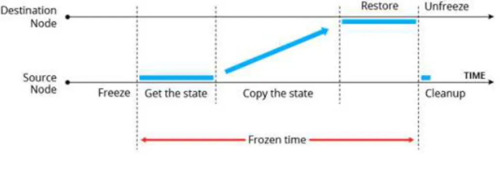
Synytsky (SYNYTSKY, 2016) described use cases for container live migration: hardware maintenance without downtime, load re-balance, HA within data centers and change of cloud vendor. The author mentioned some bottlenecks to container live migration, like applications with big amounts of data and fast changing data. Latency and data volume may be blockers to successful live migration. Figure 5describes how container live migration works.
Figure 4: VM Migration Phases.
Source:Clark et al. (2005, p. 5)
Figure 5: Container Migration Phases.
Source: Synytsky (2016, p. 3)
40 Chapter 2. Related Works
Figure 6: Container Migration Pre-Copy Memory.
Source:Synytsky (2016, p. 4)
Figure 7: Container Migration Post-Copy Memory.
Source:Synytsky (2016, p. 4)
In the pre-copy memory, during the migration process, memory from the source node is transferred to the destination until it reaches a minimum. At this point the container is frozen and the remaining data, including its state, is transferred to the destinations and the container is restored. While post-copy memory, or lazy migration, the container is frozen, the initial state is got, the fastest changing memory pages are transferred to destination and restore it. The rest of the state is copied to the destination in background mode.
Current network protocols impose significant management overhead in large data centers. Mysore et al. (MYSORE et al., 2009) proposed PortLand, a set of Ethernet compatible routing, forwarding and address resolution protocol to make management easier. They mentioned that usually data centers topology are inter connected as multi-rooted tree. Based on that, Portland employs a lightweight protocol to enable switches to discover their position in the topology. Portland uses Pseudo Mac Addresses (PMAC) to encode their position and suggests a fat tree topology. One aspect that motivated the study of server location in the data center was VM migration.
As far as monitoring is concerned, Grozev & Buyya (GROZEV; BUYYA, 2016) approached an interesting aspect, in which they do not only monitor CPU and memory, but also which VM configuration and type is more adequate for an specific application. The authors proposed a dynamic method for selecting VMs to be migrated, using machine learning techniques. In the proposed environment, the auto-scaling monitor module receives information every 5 seconds from the VMs. As far as CPU is concerned, they have collected information from the /proc/cpuinfo Linux kernel file. The objective of the auto-scaling module is to provide the ideal VM type for application servers.
The related work analysis reveals a vast study about the VM usage in the cloud environment and the growing relevance that containers are getting (RIGHTSCALE,2016). The usage of both, VM and containers, in the data center, is a solution that has shown benefits from the security standpoint and from scalability and elasticity. Real time migration is an important feature, available not only in hypervisors but also in containers, and can be used for load balancing, reduction in power consumption, disaster recovery, between others. VM solutions, like VMWare (VMWARE,2018) and Xen (XEN,2018), provide live migration mechanisms. Container live migration has evolved with the implementation of the checkpoint/restore functionality through CRIU (CRIU,2018).
This dissertation defines a heuristic that use Pearson correlation not only for CPU, but includes network traffic in the migration decision process. None of the works above mentioned takes into account CPU and network traffic at the same time. Piraghaj & Buyya (PIRAGHAJ et al., 2015) have considered only Pearson correlation coefficient for CPU in order to make a decision of which container should be migrated. Elsaid & Meinel (ELSAID; MEINEL,2014) have focused in monitoring and modeling VM live migration,
3 Pearson Correlation Model
In this Section, we describe the Pearson correlation coefficient and the heuristic developed to assist during the migration decision process. The objective of the heuristic is to determine if a VE is a good candidate to be migrated or not, considering CPU and data network traffic. By definition, a heuristic is designed to find an approximate solution, making the decision process quicker compared to complex methods that look for an exact solution.
The work of Filho & Júnior (FILHO; JÚNIOR, 2009) was the basis to explain the most important concepts of the Pearson Correlation model presented below.
3.1 Pearson Correlation Coefficient
The Pearson correlation coefficient (PEARSON,1895) estimates the dependency level between quantities. If we considern samples of two variablesx andy, represented here forxi eyi, the Pearson correlation coefficient is calculated by Equation3.1, in which ¯x and
¯
y represent the arithmetic mean of x and y, respectively. The coefficient rxy ranges from
[-1,+1] (PIRAGHAJ et al.,2015). The signal indicates the positive or negative relationship direction between variables, and the value, the strength of the relationship. When the coefficient has a value of -1 or +1, it is called a perfect correlation. Otherwise, when the coefficient has a value of 0, it means that there is no linear relation between variables.
rxy =
Pn
i=1(xi−x¯)(yi −y¯)
q Pn
i=1(xi−x¯)2Pni=1(yi−y¯)2
(3.1)
The closer the coefficient is to 1, the more dependent the variables are. When variables are dependent, they have greater probability to reach peak/valley together. Consider, for example, a VE called X and a host system Y. If the CPU correlation coefficient between X and Y is close to +1, means that CPU of VE X is contributing for a CPU peak at host Y.
Filho & Júnior (FILHO; JÚNIOR, 2009) described that the origin of the Pearson coefficient comes from the research of Karl Pearson and Francis Galton (STANTON,
2001). According to the authors, Pearson correlation coefficient r is a measure of the
44 Chapter 3. Pearson Correlation Model
that the increase or decrease of one unity in variable X generates the same impact in Y. Therefore, Pearson correlation coefficient requires shared variance, and that this variation should be distributed linearly.
In order to interpret the coefficient at this dissertation, we considered the study developed by Christine & John (CHRISTINE; JOHN,2004) that adopted the classification defined at Table1 for the coefficientr. During the interpretation of the results in Chapter 5, we will make reference to this classification. The level of association is important to our work because it will define when the CPU or network traffic of a VE is strongly associated with the host. The objective is to migrate VEs that have CPU strongly associated with the host and network traffic weakly associated.
Table 1: Pearson correlation coefficient score levels.
Coefficient Score r Classification 0.0 no relation 0.1 to 0.3 weak 0.4 to 0.6 moderate 0.7 to 1.0 strong
Source: (CHRISTINE; JOHN,2004)
The closer the score gets to 1 (independent of the signal), the greater is the linear statistical dependency degree between variables. In the opposite side, the closer to 0, the lesser is the relationship strength.
According to Filho & Júnior (FILHO; JÚNIOR,2009) the following observations can be done that are relevant for our work:
1. Pearson correlation coefficient does not differ between dependent and independent variables. Therefore, the correlation between X and Y is the same between Y and X;
2. The correlation value (score) does not change if you change the measurement unity of the variables. As an example, if you have a variable in kilograms, the score will be the same if you use grams;
3. The coefficient is dimensionless, i.e, it does not have a unity that defines it. If you have a coefficient with value r = 0.4, it cannot be interpreted as 40%, for example.
Also it can not be interpreted as been twice as strong thanr = 0.2;
4. Correlation requires that variables are quantitative;
5. The observations should be independent.
3.2 Proposed Heuristic Model
We are addressing the problem of deciding which VE to migrate based on CPU consumption and network traffic. Given that we are collecting data from the CPU con-sumption and network traffic over time, we can use the Pearson correlation coefficient presented on Section 3.1 in order to analyze if the VE resource consumption has a strong relationship with the host consumption.
Table 2 has a list of the symbols that will be used in this section with their respective definition.
Table 2: Symbol Definitions.
Symbol Definition
rCP U Pearson coefficient based on CPU
rnetwork Pearson coefficient for network (TX+RX)
rT X Pearson coefficient for TX data traffic
rRX Pearson coefficient for RX data traffic
hT X heuristic based on rCP U and rT X
hRX heuristic based on rCP U and rRX
hT ot proposed heuristic = hT X + hRX
hCP U heuristic based on CPU = rCP U
TCP U threshold for CPU consumption
T PCP U threshold for rCP U
Theuristic threshold for hT ot
CPU is an important variable in our analysis. The migration decision process starts when the CPU level reaches an established threshold. The main objective is to better load balance the workload, distributing the VEs accordingly, considering CPU and network traffic. Therefore, in our evaluation, CPU will have a higher level of importance and this will be considered while applying the heuristic. As far as the network traffic is concerned, there are two components that should be taken in consideration. The transmitted traffic (TX) and the received traffic (RX), between VEs located in the same host. As far as network traffic, the purpose is to avoid migration of VEs that exchange data with other VEs inside the same host. If we migrate such VEs, we may get an improvement in the CPU allocation, but the network traffic between hosts will increase, consuming extra network resources. The work of Morabito (MORABITO, 2015) showed the importance of considering network traffic during load balancing in order to avoid unnecessary resource consumption. Also, the extensive use of microservices technology, will create more data exchange between VEs, increasing the importance of considering network traffic during the migration process. (AMARAL et al., 2015).
46 Chapter 3. Pearson Correlation Model
was developed based on the Pearson correlation coefficient and takes into consideration the level of correlation between the host CPU and the VEs running inside the host. Furthermore, looks at the network traffic between VEs inside the host. The objective is to migrate a VE that has high correlation with host CPU but low correlation for data traffic between VEs inside the host. Therefore, we avoid migrating VEs that generate high data traffic inside the host. If we migrate such VEs, we can better distribute the load, but generate higher network data traffic between hosts. The heuristic is defined in equation
3.2:
hheuristic =
1−(weight∗rCP U)
(1 + (weight∗rCP U)−(weight∗rnetwork)) (3.2)
During simulations, the weight equals to 0.5 showed good results according to the premise of moving high correlated CPU and low correlated network traffic. Therefore, we decided to use 0.5 as the weight factor.
For network traffic, it is necessary to consider TX and RX between VEs in the same host (Figure3). To make the calculation process simpler, we decided to treat RX and TX separately, and then, add the results. Two variables were defined,hT X to calculate
the Pearson correlation coefficient for TX traffic (equation3.3) and hRX for RX traffic
(equation3.4).
hT X =
1−(0.5∗rCP U)
(1 + (0.5∗rCP U)−(0.5∗rT X)) (3.3)
hRX =
1−(0.5∗rCP U)
(1 + (0.5∗rCP U)−(0.5∗rRX)) (3.4)
At the end of the process, both calculations are added in order to generate the heuristic hT ot (equation 3.5).
hT ot =hRX +hT X (3.5)
The heuristic hT ot places a higher weight for the CPU correlation coefficient
compared to the network traffic correlation. The reason is that we only want to migrate VEs from an overloaded host, i.e, a host with high CPU and low network correlation. In order to analyze the heuristic behavior, let us look at some scenarios forhT X presented at
Table 3.
Table 3: Heuristic scores for hT X.
rCP U rT X hT X
0.0 0.0 1.00 0.0 1.0 2.00 0.3 0.3 0.85 0.6 0.6 0.70 0.7 0.0 0.48 0.7 0.6 0.62 0.7 0.7 0.65 1.0 0.0 0.33 1.0 1.0 0.50
Source: Equation 3.3
coefficient is equal to 0, there is no association between the variables, and when the coefficient is equal to 1, we have a perfect correlation. We also considered coefficients equal to 0.3 (weak association), 0.6 (moderate association) and 0.7 (strong association) (CHRISTINE; JOHN,2004). For strong associations, we also analyzed some variances in
the correlation coefficient for TX network traffic (rT X).
Let us assume that for a particular VE, the Pearson correlation coefficient for the CPU, here called rCP U, is equal or close to 0. In other words, there is no association
between the CPU consumption of the VE and the host. In this scenario, there are two alternatives regarding network traffic, one with strong relationship between VE and host (rT X >= 0.7) and the other without relationship. In the first case, if we assume a perfect
correlation (rT X = 1.0), then the score of hT X is equal to 2.00 and for the last case,
considering rT X = 0.0, the score for hT X is equal to 1.00. If we calculate the score of hT X
with weak correlations (rCP U = 0.3 andrT X = 0.3), we will get hT X = 0.85. For moderate
correlations (rCP U = 0.6 and rT X = 0.6) the score ofhT X will be 0.70. Let us look some
scenarios in which the coefficient represent strong relationship. If we look when rCP U is
equal to 0.7 (strong) and rT X = 0.6 (moderate) we got a score of 0.62 for hT X. Now if we
look when rCP U is equal to 0.7 (strong) and rT X = 0.7 (strong), the score ofhT X is equal
to 0.65. In the case of perfect association (rCP U = 1) and no association with data traffic
(rT X = 0.0), we will have a score of 0.33 for hT X. When there is association with data
traffic (rT X = 1.0), hT X will be equal to 0.50. When we compare the heuristic with the
model based on CPU only (PIRAGHAJ et al., 2015), in which migration happens when
rCP U >= 0.70, the score ofhT X will be equal to 0.48.
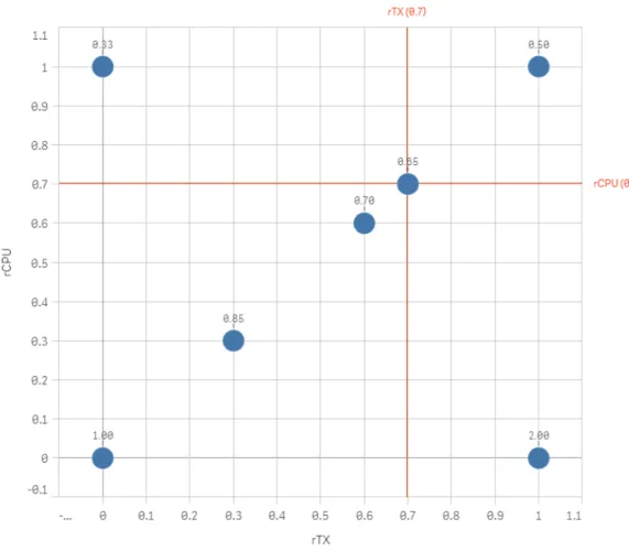
Figure8 represents the values present in Table 3.
In the y axis we haverCP U, and in the xaxis we have rT X. The value above the
plotted point is the score for hT X. Two reference lines were drawn as well, showing when
the Pearson correlation coefficient is equal to 0.70 (strong correlation). Notice that the intersection of rCP U and rT X, when the coefficients are equal to 0.70, provides a score of
48 Chapter 3. Pearson Correlation Model
Figure 8: Heuristic hT X
in most of the cases, VEs that should not be migrated. Therefore, we assume 0.65 as a threshold for hT X, meaning that values lesser or equal to 0.65 should be considered for
migration. For our test cases, results showed that the heuristic is a good approximation for most of the cases.
The same reasoning applies exactly to hRX. Therefore, the threshold for hRX is
0.65 as well.
As defined by equation 3.5, hT ot is equal to the sum of hT X and hRX. Then, the
thresholdTheuristic for hT ot is equal to 0.65 plus 0.65, resulting in a score of 1.30. If hT ot is
greater than 1.30, the module should continue with the monitoring process without any migration. Otherwise, if hT ot score is less or equal to 1.30, the VE is a candidate to be
migrated. Equation3.6 summarizes what was just described:
Heuristic=
hT ot <=Theuristic - migration
hT ot > Theuristic - do nothing
(3.6)
The heuristichT ot can be fine tuned, through changing the weightfrom equation
Theuristic, the model will be more conservative, migrating less VEs. If you increase the
threshold, the model will more flexible, migrating more VEs. Therefore, we can change the value of Theuristic to tune our model. For our tests, we will consider the threshold equals to
1.30.
3.3 Heuristic based on CPU
For comparison purposes, let us introduce a heuristic called hCP U, that will be
equal to the Pearson correlation coefficient based on CPU only, rCP U (Equation3.7). As
mentioned in Chapter 2, Piraghaj & Buyya (PIRAGHAJ et al.,2015) considered migration of containers when rCP U reaches a specific threshold. We will use the migration results
based on the score of hCP U to compare with the migrations based on hT ot.
hCP U =rCP U (3.7)
Let us define here another threshold, calledT PCP U, which establishes a threshold
for rCP U, and consequently, for hCP U. Comparing the highest coefficient of hCP U with
T PCP U, will confirm if the CPU from the VE has relationship with the CPU usage from
host. If hCP U is greater or equal than T PCP U, then there is a relationship between the
host CPU and the CPU consumption of the VE. Equation 3.8 shows the decision process.
hCP U =
hCP U < T PCP U weak relationship - do nothing
hCP U >=T PCP U strong relationship - migrate
(3.8)
4 Architecture and Implementation
This Chapter details the architecture used to validate the heuristic. It also describes how we implemented it. This implementation will be the basis for the tests accomplished in the next Chapter.
4.1 Decision/Monitoring Architecture
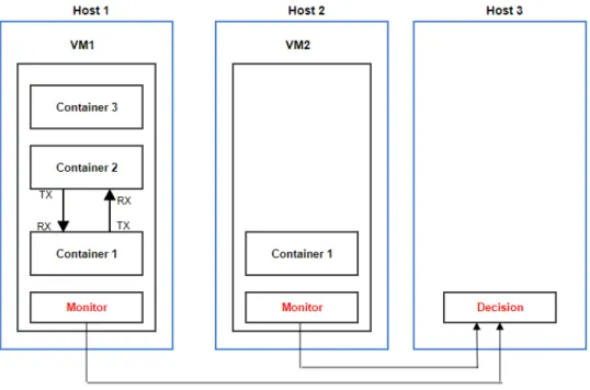
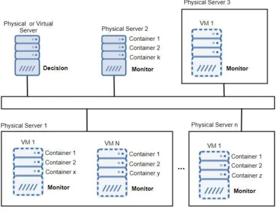
The architecture was developed to validate the proposed heuristic. It is generic in the sense that can support hosts running VMs, hosts running containers or a hybrid environment. By hybrid we consider an environment with hosts running VMs, and inside the VMs, one or more containers (CaaS model). Figure9 represents the proposed architecture and also the two main modules developed: the Decision and Monitoring modules.
Figure 9: Decision/Monitoring Scenario.
Yet, Figure 10 shows an instantiation of the architecture with different types of configurations:
Below a description of the main modules:
a. Monitor: it is responsible for collecting CPU and network data traffic statistics
52 Chapter 4. Architecture and Implementation
Figure 10: Decision/Monitoring Instantiation.
b. Decision: it receives statistics from all hosts running the Monitor Module. This
module stores the data so it can be used to calculate the Pearson correlation coefficient and apply the heuristic. When a particular host is overloaded, exceeding the established threshold, the heuristic is applied to check if there is a VE candidate to be migrated to an under-loaded host.
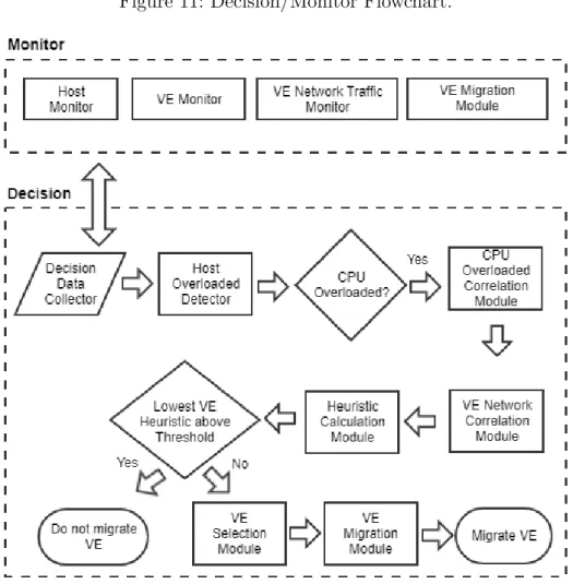
Figure 11 depicts a flowchart of the main modules and tasks executed by the Monitor and Decision modules. Following a description of each task by module.
A. Monitor Module
1. Host Monitor: it collects statistics from a host;
2. VE Monitor: it collects statistics from VEs in the host;
3. VE Network Traffic Monitor: it is responsible for collecting network traffic statistics between VEs inside the same host. It ignores the traffic that goes out; 4. VE Migration Module: it executes the commands to perform VE migration.
Figure 11: Decision/Monitor Flowchart.
54 Chapter 4. Architecture and Implementation
occur over the external network. However, if container 3 from VM1 exchanges data with container 1 of VM2, and if we transfer container 3 to host3, nothing will change in the network performance, as this traffic is already happening over the network.
The VE Migration Module executes two different tasks, one at source host and the other at destination. At source, receives the ID of the VE to be migrated and the destination host. The module executes the necessary commands to checkpoint the VE. At destination, when the VE image transfer is completed, the VE restore process takes place.
B. Decision Module
1. Decision Data Collector: it receives statistics from all hosts running the Monitor module. It stores the data so it can be later used during the Pearson correlation coefficient calculation process and to decide which host is most under-loaded to receive a migrated VE;
2. Host Overloaded Detector: after data is received by the Decision Data Collector, the CPU utilization level from the host, CP UHost, is compared to a static
threshold, called hereTCP U. IfCP UHost is less thanTCP U, then the host system
is under-loaded, otherwise, the host is overloaded. For our simulation we have set
TCP U in 70%, the same threshold value used by Piraghaj & Buyya (PIRAGHAJ
et al., 2015). Equation4.1 details the comparison:
HostCP U =
CP UHost < TCP U - under-loaded
CP UHost >=TCP U - overloaded
(4.1)
3. CPU Overloaded Correlation Module: in case that the host CPU is overloaded, the Overloaded Correlation Module is responsible for calculating the Pearson correlation coefficient between the CPU usage of every VE running in the host, and the CPU of the overloaded host (Equation 3.1). As a result, we will have a coefficient, called here rCP U, for every VE in the host. Let us define
another threshold, called T PCP U, which establishes a static threshold for rCP U.
Comparing the highest coefficient of rCP U from the host with T PCP U, will
confirm if the CPU from the VE has relationship with the CPU usage of the host. Equation4.2 summarizes the comparison. IfrCP U is greater or equal than
T PCP U, then, there is a relationship between the host CPU and the CPU usage
of the VE. This module will also store the value of rCP U for every VE, that
later will be used when applying the heuristic. Likewise, this module will create a log, registering which VE should be migrated considering rCP U only. It is
logic presented by Piraghaj & Buyya (PIRAGHAJ et al., 2015) that considers migration of containers whenrCP U reaches the threshold T PCP U. If the highest
rCP U is less or equal than the static threshold T PCP U, than the CPU usage
from the VE is not related to the CPU host consumption. Otherwise, if rCP U
is greater than T PCP U, then the CPU utilization of the VE is related to the
high CPU usage in the host. For our purpose, we will consider T PCP U greater
than 0.70 as a strong correlation (CHRISTINE; JOHN,2004). In Section 3.3
we have defined the heuristic hCP U, that is equal to rCP U.
P earsonCP U =
rCP U < T PCP U - weak relationship
rCP U >=T PCP U - strong relationship
(4.2)
Algorithm 1VE Migration Selector based on rCP U >= T PCP U
1: Input: V E_Hash, Host, CP UHost
2: Output: Hostdest, V E.M igrateID
3: if CP UHost >=TCP U then
4: V EList←host.getV EList(V E_Hash)
5: for all V Es in V EListdo
6: rCP U ← Pearson(CP UHost,CP UV E)
7: end for
8: V EM igr.rCP U ←get.HigherP earson(rCP U)
9: V E.M igrateID←get.M igrationID.HigherP earson(rCP U)
10: if V EM igr.rCP U >=T PCP U then
11: Hostdest ←host.getLowestCpuU tilization(V E_Hash)
12: Send Migration Manager (V E.M igrateID,Hostdest)
13: else
14: No migration. 15: continue; 16: end if
17: end if
Algorithm 1 receives as input a hash table with all VEs and their respective statistics per host. As output, we will have the destination host and the ID of the VE to be migrated. At line 3, we compare if the CPU of the host is overloaded, i.e, if the CPU consumption is greater or equal to the static threshold TCP U. If
it is overloaded, at line 4, VEList receives a list of the VEs for the host. Lines 5 and 6 do the Pearson’s correlation coefficient calculation for each VE in the host. Line 8 detects which VE has the highest rCP U, and, in line 9, gets the
ID of this VE. In line 10, it compares if the highest rCP U is greater or equal to
the static threshold T PCP U. If it is greater, then this VE should be migrated.
56 Chapter 4. Architecture and Implementation
migration done. If rCP U is less thanT PCP U, no migration is required. Notice
that, during this process, the network data traffic is ignored.
4. VE Network Correlation Module: This module retrieves network traffic statistics between running VEs from the overloaded host, and the objective is to verify if there is traffic between them. If internal traffic is high correlated, migration should be avoided. For the TX traffic of the VE, this module calculates the Pearson correlation coefficient rT X between the VE and all internal TX traffic
at host. The same logic is applied to RX, and the coefficient is called rRX. If
we compare the Pearson correlation coefficient to a threshold called T Pnetwork,
we can evaluate if the network traffic of a VE has a strong relationship with the host or not. For our purpose we will consider T Pnetwork greater than 0.70
as a strong correlation (CHRISTINE; JOHN, 2004). Equations 4.3 and 4.4
summarize the comparison.
P earsonT X =
rT X < T Pnetwork - weak relationship
rT X >=T Pnetwork - strong relationship
(4.3)
P earsonRX =
rRX < T Pnetwork - weak relationship
rRX >=T Pnetwork - strong relationship
(4.4)
5. Heuristic Module: previous modules have calculated the Pearson correlation coefficient for CPU and network, here called rCP U, rT X andrRX respectively.
With those values in hand, we can apply the heuristics for hT X, hRX and hT ot
and get their respectively scores (Equations 3.3, 3.4 and 3.5). The heuristic score should be compared to a static threshold, called here Theuristic. If the
lowest score forhT ot is less or equal than the static thresholdTheuristic, then the
VE is the one that should be migrated. Otherwise, if hT ot score is greater than
Theuristic, then the VE should not be migrated as there is considerably internal
traffic between VEs inside the same host. A heuristic is an approximation of the exact solution. Note that if Theuristic is defined too low, the model will be
very restrictive, allowing few migrations. Otherwise, if defined too high, the model will be very flexible, allowing more migrations. As defined in Section
3.2, we will work with Theuristic equals to 1.30. Equations 4.5summarizes the
explanation. Heuristic=
hT ot <=Theuristic - migrate
hT ot > Theuristic - do not migrate
(4.5)