Onset detection in music signals

(1)

Department of Information Science and Technology

Onset Detection in Music Signals

Carlos Manuel Tadeia Ros˜ao

A Dissertation presented in partial fulfilment of the Requirements for the Degree of Master in Open Source Software (Software de C´odigo Aberto)

Supervisor:

Doctor Ricardo Daniel Santos Faro Marques Ribeiro, Assistant Professor, ISCTE-Instituto Universit´ario de Lisboa

Co-supervisor:

Doctor David Manuel Martins de Matos, Assistant Professor, Instituto Superior T´ecnico, Universidade T´ecnica de Lisboa

(2)

(3)

Department of Information Science and Technology

Onset Detection in Music Signals

Carlos Manuel Tadeia Ros˜ao

A Dissertation presented in partial fulfilment of the Requirements for the Degree of Master in Open Source Software (Software de C´odigo Aberto)

Supervisor:

Doctor Ricardo Daniel Santos Faro Marques Ribeiro, Assistant Professor, ISCTE-Instituto Universit´ario de Lisboa

Co-supervisor:

Doctor David Manuel Martins de Matos, Assistant Professor, Instituto Superior T´ecnico, Universidade T´ecnica de Lisboa

(4)

(5)

(6)

(7)

Resumo

A Deteçcão de Onsets, ou seja, a tarefa que procura encontrar o momento de in´ıcio de notas musicais num sinal de áudio, tem sido uma área de investiga¸cão activa, uma vez que a De-teçcão de Onsets é comummente utilizada como primeiro passo em tarefas de alto-n´ıvel de processamento musical.

Tendo em conta a necessidade de saber que método de Deteçcão de Onsets é mais adequado a cada tarefa de alto-n´ıvel, nesta tese foram seguidas duas abordagens que visam, acima de tudo, obter uma informa¸cão mais completa sobre cada método de Deteçcão de Onsets.

A primeira abordagem consiste numa compara¸cão em profundidade do comportamento dos métodos de Deteçcão de Onsets que usam caracter´ısticas espectrais do sinal. Os resultados obtidos mostram que o comportamento dos diferentes métodos varia significativamente entre as fun¸cões de deteçcão usadas, entre os tipos de Onset, e ainda de acordo com a técnica de interpreta¸cão do instrumento.

Na segunda abordagem avalia-se a influência do passo final de Seleçcão de Picos nos resultados globais de Deteçcão de Onsets. Os resultados obtidos mostram que o passo de Seleçcão de Picos influencia profundamente os resultados – negativa e positivamente –, e que esta influência difere significativamente de acordo com o tipo de Onset e com o método de Deteçcão de Onsets usado.

(8)

(9)

Abstract

Onset Detection, that is, the quest for finding the starting moment of musical notes in an audio signal, is an active research subject since note onset detection is commonly used as a first step in high-level music processing tasks.

Driven by the need to know which Onset Detection method can suit better each high-level music processing task, two approaches are followed in this thesis in order to obtain a more complete information about the different onset detection methods.

The first consists in a full comparison of the performance of Onset Detection Methods that use Spectral Features. Our results in two distinct datasets show that the behaviour of onset detection varies clearly between onset types and between detection functions, as well as between instrument interpretation style.

The other approach assesses the influence of the final Peak Selection step in the global re-sults of Onset Detection. Our rere-sults show that the Peak Selection step used deeply influences both positively and negatively the results obtained, and that its influence differs significantly according to the onset classes and to the onset detection functions.

(10)

(11)

Palavras Chave

Keywords

Palavras Chave

Detec¸c˜ao de Onsets

Segmenta¸cão de Notas Musicais Capta¸cão de Informa¸cão Musical Transcri¸cão Musical Automática Deteçcão de Novidade

Processamento de Sinal

Keywords

Onset Detection Note Segmentation

Music Information Retrieval Automatic Music Transcription Novelty Detection

(12)

(13)

Acknowledgements

I would like to thank to my supervisors Ricardo Ribeiro and David Martins de Matos for all the helpful discussions and fruitful advices.

Another thank goes to Professors Carlos Costa and Manuela Apar´ıcio for all their advices and guidance during the completion of the master course.

A great thank you goes also to my colleagues in the Master in Open Source Software, who pointed some interesting questions concerning the subject of my thesis.

I would like also to thank my friends for being there for me.

Finally, I am most grateful to my family, especially my mother, grand-mother and brother for all the invaluable support and for sharing with me the taste for learning.

Lisboa, Abril 30, 2012 Carlos Manuel Tadeia Ros˜ao

(14)

(15)

“Music is a moral law. It gives soul to the universe, wings to the mind,

flight to the imagination, and charm and gaiety to life and to

everything”

Plato

(16)

(17)

List of Figures

2.1 Attack, onset and transient in a single note. . . 6

2.2 Polyphonies – (a)synchronous onsets. . . 7

2.3 An onset produced by a clarinet, as an example of extended transient. . . 8

2.4 The glissando as an example of an ambiguous onset. . . 8

2.5 Traditional onset detection work-flow. . . 10

2.6 Time vs Amplitude and Time vs Spectral Magnitude representation of piano notes. . . 12

2.7 High Frequency Content, Signal, and Spectrogram for 1s of a PP song from the Bello Dataset. . . 14

2.8 Spectral Flux and Signal for 1s of a PP song from the Bello Dataset. . . 15

2.9 Phase Deviation and Signal for 1s of a PP song from the Bello Dataset. . . . 18

2.10 Complex Domain and Signal for 1s of a PP song from the Bello Dataset. . . . 19

2.11 Filter classification. . . 23

2.12 Constant threshold. . . 24

2.13 Running-mean adaptive threshold. . . 26

3.1 Relationship between the quantities defined in the Classification Matrix. . . . 30 3.2 Precision vs Recall for the SF OSS in all the onset classes of the Bello Dataset. 35 3.3 Precision vs Recall for the RCD OSS in all the onset classes of the Bello Dataset. 37

(20)

(21)

List of Tables

3.1 Classification Matrix . . . 29

3.2 Alicante Dataset Structure . . . 32

3.3 Bello Dataset Structure . . . 32

3.4 Overal Results by OSS in the Alicante Dataset . . . 34

3.5 Overal Results by OSS in the Bello Dataset . . . 34

3.6 Results for the Alicante Dataset: Precision(P), Recall(R), and F-measure(F) 34 3.7 Results for NPP and PP onset classes in the Bello Dataset: Precision(P), Recall(R), and F-measure(F) . . . 34

3.8 Results for PNP and Mix onset classes in the Bello Dataset: Precision(P), Recall(R), and F-measure(F) . . . 34

3.9 Top 5 results for violin song 1 - common interpretation . . . 39

3.10 Top 5 results for violin song 2 - virtuoso interpretation . . . 39

3.11 Components of the Peak Selection Methods A, B, C, D and E. . . 41

3.12 Results for NPP onsets in the Bello Dataset using the Peak Selection methods A, B, and C: P, Precision, F, F-measure and R, Recall. . . 41

3.13 Results for NPP onsets in the Bello Dataset using the Peak Selection methods D and E: P, Precision, F, F-measure and R, Recall. . . 42

3.14 Results for PP onsets in the Bello Dataset using the Peak Selection methods A, B, and C: P, Precision, F, F-measure and R, Recall. . . 42

3.15 Results for PP onsets in the Bello Dataset using the Peak Selection methods D and E: P, Precision, F, F-measure and R, Recall. . . 43

3.16 Results for PNP onsets in the Bello Dataset using the Peak Selection methods A,B, and C: P, Precision, F, F-measure and R, Recall. . . 43

3.17 Results for PNP onsets in the Bello Dataset using the Peak Selection methods D and E: P, Precision, F, F-measure and R, Recall. . . 44

3.18 Results for Mix onsets in the Bello Dataset using the Peak Selection methods A, B, and C: P, Precision, F, F-measure and R, Recall. . . 44

3.19 Results for Mix onsets in the Bello Dataset using the Peak Selection methods D and E: P, Precision, F, F-measure and R, Recall. . . 44

(22)

(23)

1

Introduction

1.1 Context & Motivation

It is thought that music appeared between 60.000 and 30.000 years ago (Wallin et al., 2001) when humans started creating several art forms such as painting and jewellery. On the other hand, there is no general agreement in the precise form it appeared. Some suggest that its origin is based on natural occurring sounds and rhythms while others suggest its origin is related to hunting purposes (Wallin et al., 2001).

The sound, and specifically music, have been present in the human life since music was discovered, thus it is no surprise that humans have an innate capacity to understand some of its elements (tone, rhythm, dynamic, texture).

Music has been the subject of study and research for at least more than two millennia. Pythagoras, 2.500 years ago, is usually credited with the first studies in proportion and harmony (Abraham, 1979).

The study of music has continued throughout the centuries, although in the past 50 years, with the fast advances in computers and digitalization, new means were created to aid this study (Casey et al., 2008), which led to faster and in-depth advancements. More recently, when music downloaded over the internet outsold music in CD format, the music industry turned its way even more to music in digitalized format which created an exponential growth in research on this area (Casey et al., 2008).

The work presented with this thesis is part of the broad area of Music Information Re-trieval (MIR). MIR is a recent and emerging research area devoted to fulfil the listeners’ music information needs (Orio, 2006). That is, it aims at finding and retrieving relevant informa-tion to humans from the musical signal. This informainforma-tion is not necessarily a mathematical property of the music, such as pitch or tempo, it can also be a “psychological property” of

(24)

the music, such as musical style or mood (Orio, 2006).

In this thesis, we are mainly concerned with Onset Detection, a very specific subject within the MIR broad area. In a very general way, Onset Detection deals with finding the starting moments of notes in an musical audio signal (Dixon, 2006)1.

Onset Detection has innumerable applications. It can be used as the first step for segmen-tation (Duxbury, Bello, Davies, & Sandler, 2003), beat tracking (Davies & Plumbley, 2007) and query by humming (Ding et al., 2011). It can also be used as the basis for the retrieval of many high level musical features (Eyben et al., 2010), such as Chord Estimation, Harmonic Description or Music Genre Classification (Davies & Plumbley, 2007), which allows one to make content-based querying and retrieval (Casey et al., 2008).

Onset Detection can even be applied to Biology, as was done by the pioneering work of Barthet et al. (2010). In this work, onset detection methods were used to analyse the calcium activity in zebrafish (tropical freshwater fish) living embryos.

1.2 Objectives

The main purpose of the work described in this thesis is to explore the most common methods of Onset Detection, trying to understand how their results vary according to the musical type, and which factors influence most their performance.

Two different but complimentary research directions are followed: a comparison of six different Onset Detection Methods and a study in how the Peak Selection step of Onset Detection influences its results.

Both these approaches aim at providing the most complete information about the different Onset Detection methods, that is, how the results of different Onset Detection methods differ amongst themselves, according to the musical type, and which Peak Selection Method suits best each Onset Detection method.

This information can be of great help to someone who wants to use Onset Detection for a particular application – query by humming or segmentation, to name just two examples – and does not know which method suits best his needs.

1

(25)

1.3. THESIS CONTRIBUTIONS 3

1.3 Thesis Contributions

The outcome of this work consists mainly of five contributions:

state of the art - A vast introduction and explanation of the most common Onset Detection Methods that make use of many types of tools: from Time-domain analysis, to Machine-learning approach, passing through the Spectral Domain analysis.

comparison of onset detection methods - A full comparison of the results of six distinct Onset Detection Methods that use Spectral Features.

influence of violin interpretation style on onset detection - A comparison of the in-fluence of violin interpretation style in the results of Onset Detection Methods.

analysis of the peak selection influence on onset detection - A deep study of the in-fluence of five of the most common peak selection techniques in the results of Onset Detection.

open source framework for audio analysis - In order to explore and test the results of the different Onset Detection methods, an audio-framework was build with the Java programming language and made freely available 2_.

1.4 Related Publications

Alongside the development of the thesis, three papers were produced:

• Ros˜ao, C. & Ribeiro, R. (2011). Trends in Onset Detection. In Proceedings of the 2011 Workshop on Open Source and Design of Communication. ACM.

• Ros˜ao, C., Ribeiro, R., & de Matos, D. Martins. (2012). Comparing Onset Detection Methods Based on Spectral Features. In Proceedings of the 2012 Workshop on Open Source and Design of Communication. ACM.

2

(26)

• Ros˜ao, C., Ribeiro, R., & de Matos, D. Martins. (2012). Influence of Peak Selection Methods in Onset Detection. In Proceedings of the 13th International Society for Music Information Retrieval Conference (ISMIR 2012).

1.5 Outline of the Thesis

This document is organized as follows:

Chapter 1 introduces our aims and gives an overview of the worked developed in the thesis and its contributions.

Chapter 2 gives a general overview of the Onset Detection area. It starts with a musi-cal introduction that helps defining clearly an onset and the different onset classes. Next, the complete process that leads from the audio signal to the onsets is explained. The most common onset detection techniques are grouped by Time-domain, Spectral-domain, Probabilistic, Pitch-based, and Data-driven. Each of the groups is explained mathematically and its strengths and weaknesses introduced. The chapter ends with an overview of the most common peak selection methods.

Chapter 3 explains, evaluates and discusses the results of the different experiments made. It starts by defining the datasets used as well as the evaluation methods that are used to analyse the results. Next, it explains the experiments and discusses the results in three disctinct parts: Comparison of Onset Detection Methods, Influence of Interpretation Style and Influence of Peak Selection Methods.

Chapter 4 concludes this thesis: final conclusions are presented, the contributions of the work developed are revisited, and possible directions for future work are enumerated.

(27)

2

Onset Detection

The history of onset detection using computers can be traced back to the 1980’s when several algorithms, such as the one presented by Schloss (1985), were proposed to find the beats in music signals composed solely of percussion.

However, only in the 1990’s Goto & Muraoka (1994) proposed the first algorithm aimed at finding the rhythm of a general audio signal.

Since the 1990’s, as the available computational power increased, the interest in music transcription has grown rapidly and several different algorithms to find onsets in music signals were developed (Klapuri & Davy, 2006).

Before introducing the most common Onset Detection Techniques, one must define pre-cisely what an onset is. In order to do so, a short musical introduction is required.

2.1 Definitions

2.1.1 Musical Introduction

In a general way, music is composed by sounds generated simultaneously by several musical instruments of different kinds (Klapuri & Davy, 2006). Thus, one can consider the notes played by these musical instruments as the basic unit for a musical signal.

Notes can be categorized as harmonic or percussive. Harmonic are the ones which humans would categorize as musical notes, because they have a well defined pitch and harmonically related partials (Klapuri & Davy, 2006). On the other hand, percussive notes, do not have a defined pitch, being analogous to noise clouds (Klapuri & Davy, 2006).

(28)

2.1.2 Onset

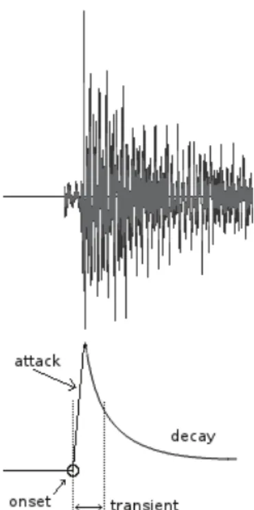
There are several equivalent ways of defining an onset. One can define it as the start of a musical note (not restricting notes to those having a clearly defined pitch) (Dixon, 2006), the starting moment of an acoustic event (Eyben et al., 2010), or as a single instant chosen to mark the temporally extended transient (Bello et al., 2005). The transient can be understood as a short-time interval in which a significant energy change occurs in the signal (Bello et al., 2005; Klapuri & Davy, 2006).

For the ideal case of a single musical note, one can see a clear definition of these concepts in the schema present in Fig. 2.1.

Figure 2.1: Attack, onset and transient in a single note (Bello et al., 2005).

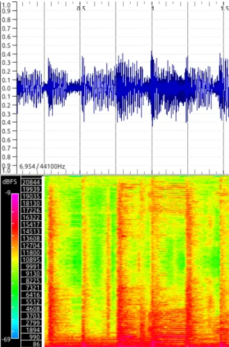
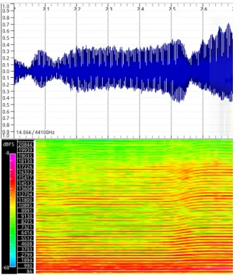
At first sight, an onset seems like a very well-defined concept, although the definition becomes blurred when dealing with polyphonies (see Fig. 2.2) where chords are played “syn-chronously” (Dixon, 2006) – the start of the notes that compose a chord might spread by tenths of milliseconds – or when we have instruments with long attack times (clarinet for instance) which produce extended transients (see Fig. 2.3), or even when we have certain

(29)

2.1. DEFINITIONS 7

Figure 2.2: Polyphonies – (a)synchronous onsets (signal on top and spectrogram on bottom)

performance techniques such as glissando, tremolo or vibrato (see Fig. 2.4).

To overcome this ambiguities in defining precisely an onset, usually the definition of onset is suited to particular applications (Dixon, 2006).

2.1.3 Onset Classes

As we have seen in Section 2.1.2, we can consider an onset as the starting moment of a musical note, in this way it is possible to categorize onsets the same way we have categorized notes in Section 2.1.1.

Hence, we can distinguish the following onset classes: • Non-pitched Percussive (NPP);

(30)

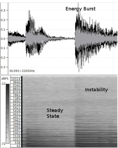
Figure 2.3: An onset produced by a clarinet, as an example of extended transient (signal on top and spectrogram on bottom)

Figure 2.4: The glissando as an example of an ambiguous onset (signal on top and spectrogram on bottom)

(31)

2.2. ONSET DETECTION METHODS 9 • Pitched non-percussive (PNP); and,

• Complex Mixtures (Mix).

One can think of Complex Mixture as any polyphonic music where several instruments are played together, something that happens, for instance, in a rock or pop song. The NPP onsets are the ones typically produced by percussion instruments such as drums or cymbals, while the PP onsets are those that have a percussive characteristic but, nonetheless, still maintain a well defined pitch; these onsets appear, for instance, when a piano is playing. Finally, the PNP onsets are those that do not have percussive characteristics and have a very well defined pitch; this category contains onsets from instruments such as bowed strings or wind instruments.

2.2 Onset Detection Methods

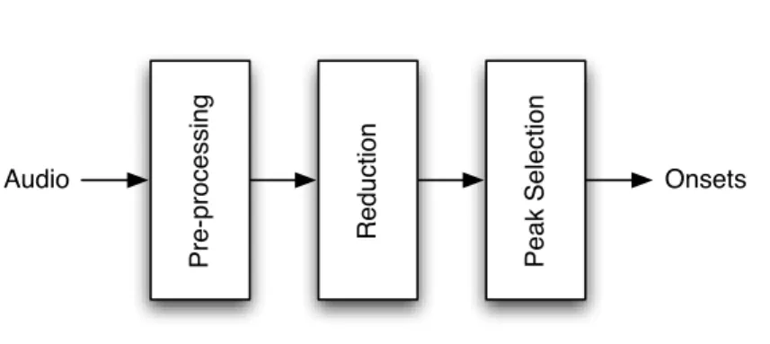
Most of the existing Onset Detection algorithms follow a general pattern, depicted in Fig. 2.5, which comprises the following steps (Bello et al., 2005; Eyben et al., 2010; Holzapfel et al., 2010):

1. Preprocessing of the raw audio signal in order to improve the performance of later stages;

2. Computation of a detection function1, i.e., a function whose peaks should be simulta-neous, within a tolerance margin, with onset times (Dixon, 2006); and,

3. Application of a peak-picking algorithm to the detection function in order to select the appropriate peaks.

2.2.1 Preprocessing

Preprocessing is an optional step that transforms the original signal aiming to emphasize its most important properties to onset detection (Bello et al., 2005; Eyben et al., 2010).

1

In the literature, other terms are also used to denote detection function, for instance Ellis (2007) uses onset strength signal (OSS) and Foote (2007) uses audio novelty. The term audio novelty comes from the novelty function, very common to the literature in machine learning and communication theory.

(32)

Pre -p ro ce ssi n g Pe a k Se le ct io n R e d u ct io n Audio Onsets

Figure 2.5: Traditional onset detection work-flow (Eyben et al., 2010).

The most common pre-processing methods consist in separating the signal into multiple frequency bands and transient/steady-state separation (Bello et al., 2005). As an example, the algorithms proposed by Goto & Muraoka (1996) and by Scheirer (1998) both use the separation of the original signal in multiple frequency bands. Despite being commonly related to music modelling (Bello et al., 2005), the process of transient/steady-state separation can also be used as a pre-processing method for onset detection; Duxbury et al. (2001) used this possibility in the development of an onset detection method.

There is yet another very common pre-processing method called Adaptive Whitening. This method was proposes by Stowell & Plumbley (2007) and consists in normalising the magnitude of each bin according to a recent maximum, aiming to mitigate the influence of the strong dynamics of most musical audio signals (Stowell & Plumbley, 2007).

2.2.2 Detection Function

A detection function is aimed at detecting changes in the properties of an audio signal (Dixon, 2006), by simplifying it (lowering the sample rate, for instance), but maintaining the impor-tant information. Thus, a detection function is the result of a process, sometimes called Reduction, that transforms the original signal into a more simplified function which easily expresses the transients (Bello et al., 2005).

During the years, many detection functions have been proposed. In spite of analysing every approach separately, one can group them in several groups according to their properties. Thus, we have (Eyben et al., 2010): time domain reduction functions, spectral domain reduction functions, probabilistic reduction functions, pitch-based onset detection techniques and

(33)

data-2.2. ONSET DETECTION METHODS 11 driven reduction functions.

2.2.2.1 Time domain reduction functions

Typically, an onset corresponds to an increase in the signal’s amplitude (Bello et al., 2005). Early methods, such as the one proposed by Schloss (1985), picked this concept and analysed the amplitude envelope of the signal, obtaining satisfactory results on music with intense percussive transients. This envelop can be obtained by:

E0(n) = N 2−1 X m=−N₂ |x(n + m)|w(m) (2.1)

where x is the signal function and w(m) is an N -point rectangular window.

There is an improvement of this method in which the local energy is followed instead of the amplitude: E(n) = N 2−1 X m=−N₂ [x(n + m)]2w(m) (2.2)

It is possible to further refine this method by analysing the time derivative of the energy and not the energy itself. In this way bursts of energy are converted to peaks in the derivative function (Bello et al., 2005). There is yet another possible refinement which is based on experimental clues that loudness is perceived logarithmically by the human hear (Moore et al., 1997). Accordingly to Klapuri (1999), this strategy causes a better elimination of false onsets. Thus, this method uses the following equation, for the relative difference function W , to mimic the human ear perception of loudness (Klapuri, 1999):

W = d

dt(log(E(t))) =

dE dt

E (2.3)

2.2.2.2 Spectral domain reduction functions

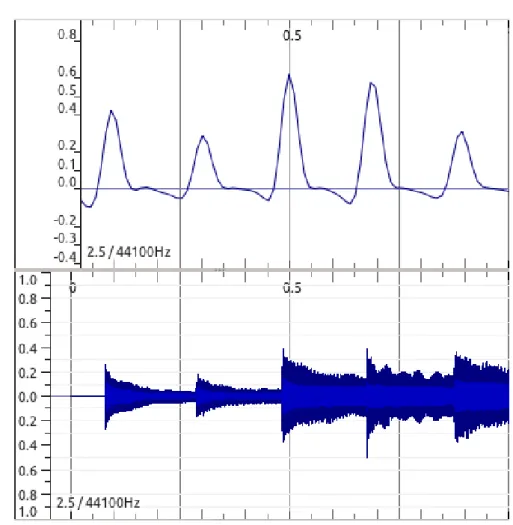
Instead of analysing the time domain of a signal, recent systems employ reduction functions that work in the spectral domain (Eyben et al., 2010). In Fig. 2.6 one can see this two representations for the same excerpt of piano music.

(34)

Figure 2.6: Time vs Amplitude (top) and Time vs Spectral Magnitude (bottom) representa-tion of piano notes.

In the following paragraphs we will briefly explain several onset detection methods be-longing to the group of spectral domain reduction functions. Note that the methods listed in this subsection are all based on a STFT of the signal, that for a general signal x(n) and the nth _{bin of the k}th _{frequency can be defined as:}

Xk(n) = N 2−1 X m=−N₂ [x(nh + m)]2w(m)e−−2iπmkN (2.4)

where w(m) represents an N -point rectangular window and h the hop-size, i.e., the time-shift between adjacent windows.

(35)

2.2. ONSET DETECTION METHODS 13 frequency components in the spectrogram (Klapuri & Davy, 2006):

E(n) = 1 N N 2−1 X k=−N₂ |X_k(n)|2 (2.5)

2.2.2.2.1 High frequency content By observing that an energy increase in one or more frequency bands can be a simple indicator of an onset (Dixon, 2006), one can notice that an onset has a more intense energy in the bands in which the interference with other simultaneous components is smaller (Dixon, 2006), a situation which typically occurs in the high-frequencies region (Rodet & Jaillet, 2001; Bello et al., 2005). This fact can be exploited by weighting each STFT bin with a factor proportional to its frequency. Hence, by summing all weighted bins, one obtains a function called HFC or eE – see Fig. 2.7 –, that can be used as detection function: HF C(n) = 1 N N 2−1 X k=−N₂ Wk|Xk(n)|2 (2.6)

where Wk represents the frequency dependent weighting.

The authors Masri (1996) and Masri & Bateman (1996) proposed a linear weighting of the frequencies with Wk = |k|. Although this method works well for percussive onsets, it shows

weaknesses for other onset types (Bello et al., 2005).

Later, Rodet & Jaillet (2001), proposed a similar method and obtained good results for high-frequencies, thus showing consistency with Masri’s idea.

2.2.2.2.2 Spectral Difference There is a more general approach based in spectral changes of the signal, and is related to the formulation of the detection function as a “dis-tance” between successive STFT, treating them as points in an N -dimensional space (Bello et al., 2005). According to the distance function used, the detection function receives different names:

1. If using the L1-norm as a distance function, then, the detection function is called SF (Dixon, 2006; Masri, 1996) – see Fig. 2.8;

(36)

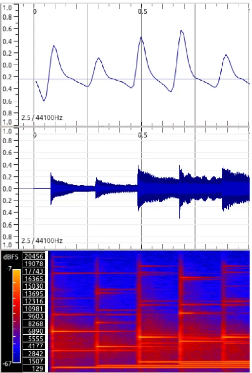
di-Figure 2.7: High Frequency Content (top), Signal (middle), and Spectrogram (bottom) for 1s of a PP song from the Bello Dataset.

(37)

2.2. ONSET DETECTION METHODS 15 vergence, then, the detection function is called SD (Duxbury et al. (2002) developed an algorithm that uses this distance function).

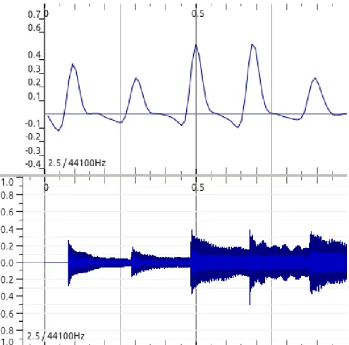
Figure 2.8: Spectral Flux (top) and Signal (bottom) for 1s of a PP song from the Bello Dataset.

Dixon (2006) showed that the results with the L1-norm outperform those with the L2-norm. Nonetheless, in any of the cases, the function measures the change in magnitude in each frequency bin (Dixon, 2006) and is calculated by computing the difference of two consecutive short-time spectra bin by bin (Eyben et al., 2010) (using any of the distance functions referred above to calculate the difference). With the L1-norm it becomes:

SF (n) = N 2−1 X k=−N₂ H(|Xk(n)| − |Xk(n − 1)|) (2.7)

(38)

and with the L2-norm it takes the form: SDL2(n) = N 2−1 X k=−N₂ {H(|X_k(n)| − |Xk(n − 1)|)}2 (2.8)

where H(x) = x+|x|₂ is called the half-wave rectifier function (Dixon, 2006) and has the purpose of eliminating negative differences. In this way, it ignores offsets and sticks to onsets.

There is also a related form of Spectral Difference function introduced by Foote (2007), which uses the correlation between STFT to be calculated. However, according to Bello et al. (2005), this approach is only effective when small width windows are used in its calculus. The methods using Spectral Difference or Spectral Flux give very good results in finding NPP onsets (Bello et al., 2005). Furthermore, these methods have proved to be among the best overall performers so far (Eyben et al., 2010), so it is not surprising to see many studies using them (Holzapfel et al., 2010), like, for instance, the works of Hainsworth & Macleod (2003), Collins (2005a) and Dixon (2006).

2.2.2.2.3 Phase deviation The methods we have seen so far use the magnitude of the spectrum as their source of information, however, in recent years, several studies make use of the phase spectra. This type of analysis is also important, because much of the temporal structure of a signal is contained in the phase spectrum (Bello et al., 2005).

Let φk(n) be the phase of the transformed signal Xk(n), i.e., respects the relation:

Xk(n) = |Xk(n)|eiφk(n) (2.9)

where φ is mapped onto the range ] − π, π].

It is unlikely that the frequency components of the new sound are in phase with the previous sound, so irregularities in the phase of several frequency bins can be used to indicate the presence of onsets (Dixon, 2006). According to Eyben et al. (2010), the change of the phase in a STFT frequency bin is a rough estimate of its instantaneous frequency, and can be used as indicator of an onset.

(39)

2.2. ONSET DETECTION METHODS 17 signals), so, one can write the instantaneous frequency as:

φ0_k(n) = φk(n) − φk(n − 1) (2.10)

And the variation of the instantaneous frequency as:

φ00_k(n) = φ0_k(n) − φ0_k(n − 1) (2.11)

In 2003, Bello & Sandler (2003), proposed an algorithm that analyses the distribution of phase deviations across all frequencies. Later in the same year, Duxbury, Bello, Davies, & Sandler (2003) proposed a simpler measure of the spread of the previous distribution, denoted by PD:

P D(n) = 1 N N 2−1 X k=−N₂ |φ00_k(n)| (2.12)

A few years later, Dixon (2006) proposed a refinement of the previous method, so it can account for “noise introduced by components with no significant energy” (Bello et al., 2005). The PD considers all frequencies equally, so Dixon (2006) proposed weighting the frequency bins by their magnitude, in order to obtain a new onset detection function which he named WPD: W P D(n) = 1 N N 2−1 X k=−N₂ |X_k(n)φ00_k(n)| (2.13)

where Xk(n) represents the magnitude.

A further option is to normalize the previous equation, obtaining a NWPD function:

N W P D(n) = PN2−1 k=−N₂ |Xk(n)φ 00 k(n)| PN2−1 k=−N₂ |Xk(n)| (2.14)

These methods based on phase deviation tend to give better results on PNP onsets than the methods that use the spectral magnitude (Bello et al., 2005), though, in NPP onsets the results are not as good as the ones obtained with the other type of methods.

(40)

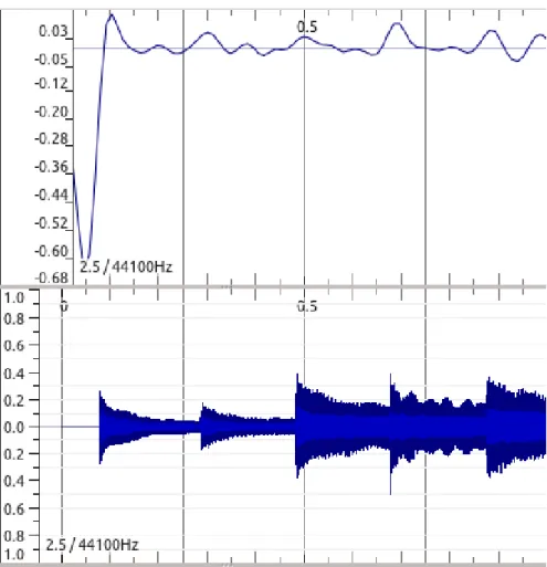
Figure 2.9: Phase Deviation (top) and Signal (bottom) for 1s of a PP song from the Bello Dataset.

2.2.2.2.4 Complex domain Like in the previously defined WPD and NWPD functions, one can combine both energy and phase information for the production of a CD func-tion (Duxbury, Bello, Davies, & Sandler, 2003).

In this way, amplitude and energy are used together to check for irregularities in the steady state (Dixon, 2006). A method that uses this concept was first proposed by Duxbury, Bello, Davies, Sandler, & Others (2003), and later extended by Bello et al. (2004).

A few years later, Dixon (2006) made an equivalent, but simpler formulation, of Bello’s approach. He defined the CD as:

CD(n) = 1 N N 2−1 X k=−N₂ |Xk(n) − ˜Xk(n)| (2.15)

(41)

2.2. ONSET DETECTION METHODS 19 where Xk is the amplitude and phase of the current bin, based on the previous two bins,

and ˜Xk is the target value, i.e., the value predicted by the previous frames. The prediction

assumes constant amplitude and rate of phase change:

˜

Xk(n) = |Xk(n − 1)|ei(φk(n−1)+φ

0

k(n−1)) (2.16)

All in all, this method sums the magnitude of the complex differences between the actual values for each frequency bin and the estimated ones, and uses the result as a detection function.

In Fig. 2.10 we see a representation of this OSS.

Figure 2.10: Complex Domain (top) and Signal (bottom) for 1s of a PP song from the Bello Dataset.

(42)

so in 2006 he proposed a RCD function to surpass this problem. This method uses a half-wave rectification (similar to the SF method) in order to preserve only the positive variations of energy in the spectral bins. Hence, the RCD is defined as:

RCD(n) = N 2−1 X k=−N₂ RCDk(n) (2.17) where RCDk(n) =            |X_k(n) − ˜Xk(n)| if |Xk(n)| > |Xk(n − 1)| 0 otherwise (2.18)

Although being a little harder to implement, these kind of methods show very good results in the detection of both NPP and PNP onsets (Bello et al., 2005).

2.2.2.3 Probabilistic reduction functions

An alternative to the previous models is to base the description of the signals on probabilis-tic/statistical methods, i.e., assuming that the signal can be described by some probabilistic model and to look for abrupt difference between the model and the “real signal”. Obviously, the success of this approach is dependent on the degree of closeness between the model and the “real signal”. This type of similarity can be quantified using measures of likelihood or Bayesian model selection criteria (Bello et al., 2005).

Every statistical method of this kind follows one of two main strategies:

1. Approaches Based on “Surprise Signals” — the strategy here is to look for a sudden change (surprise signal) of a particular global model that is assumed to describe the signal (Bello et al., 2005);

2. Model-Based Change Point Detection Methods — in this case, the goal is to observe which of the two previously defined probability models the system follows (Eyben et al., 2010).

(43)

2.2. ONSET DETECTION METHODS 21 is an example of a model based on “surprise signals” and shows very good results in music with non-percussive onsets (Bello et al., 2005). On the other hand, the sequential probability ratio test, applied, for instance by Basseville & Nikiforov (1993), is a good example of the utility of the second strategy.

The statistical onset detection methods have the peculiarity of providing very good results in the discovery of non-percussive onsets (Bello et al., 2005).

2.2.2.4 Pitch-based onset detection techniques

Pitch is a perceived sound property closely related to frequency that allows one to organize sounds in a frequency-related scale, i.e., with notions of “higher” and “lower” in the com-mon way associated with melody (Klapuri & Davy, 2006). This means that pitch is not a physical property of sound, it is a subjective property, commonly studied in the area of psychoachoustics.

The physical concept closer to pitch is the fundamental frequency, f0, though, for

poly-phonic music signals, there are some dificulties in finding the value of this property (Klapuri & Davy, 2006). Pitch-based onset detection methods use the concept of pitch contour, i.e., the variation in time of the fundamental frequency, and assume that discontinuities and abrupt changes in this function indicate the presence of onsets (Eyben et al., 2010). Hence, pitch-based onset detectors are pitch-based on finding these kind of discontinuities and abrupt changes in the pitch contour (Collins, 2005b).

Several algorithms were proposed, for instance, the works of Collins (2005b) or Zhou & Reiss (2007), that use this kind of strategy, and according to the comparative study performed by Bello et al. (2005), they show better results in PNP onsets than the algorithms based in the magnitude of the spectrum (Collins, 2005b).

2.2.2.5 Data-driven reduction functions

One of the difficulties that the previous methods have shown is that they perform well only for certain types of music: performance diminishes when range of music signals increases (Eyben et al., 2010).

(44)

In order to try to overcome this limitation, data-driven reduction functions have been proposed.

These functions tend to depend on machine-learning algorithms, such as neural networks and some of them have great performance in a large spectrum of music types. For instance, La-coste & Eck (2005) is based on a feed forward neural network and achieved the best perfor-mance in the Mirex 2005 audio onset detection evaluation (MIREX, 2005), and Eyben et al. (2010) uses a bidirectional Long Short-Term Memory recurrent neural network and was the algorithm which performed best in the Mirex 2010 audio onset detection evaluation (MIREX, 2010).

Statistical methods seem to have the best overall performance. However, computational requirements and the need of a training corpus may difficult their application (Bello et al., 2005).

2.2.3 Peak Selection

A detection function created with any of the above methods shows well localized maxima, generally with some variability due to noise (Bello et al., 2005). In order to pick the onsets from the detection function, several steps are used that typically fit in the following categories: Post-processing, Thresholding and Peak-picking.

2.2.3.1 Post-processing

Post-processing deals with simplifying the subsequent processes of thresholding and peak picking by increasing the uniformity in the detection function (Bello et al., 2005). This process of increasing the uniformity of the detection function typically makes use of normalization methods and filters.

The normalization typically works in one of two ways (Dixon, 2006; Holzapfel et al., 2010):

• Subtract the average value of the function from each value, so that the average will be zero and then divide by the maximum value so that the function will be in the interval [-1,1] (later we will call this normalization method by norm).

(45)

2.2. ONSET DETECTION METHODS 23

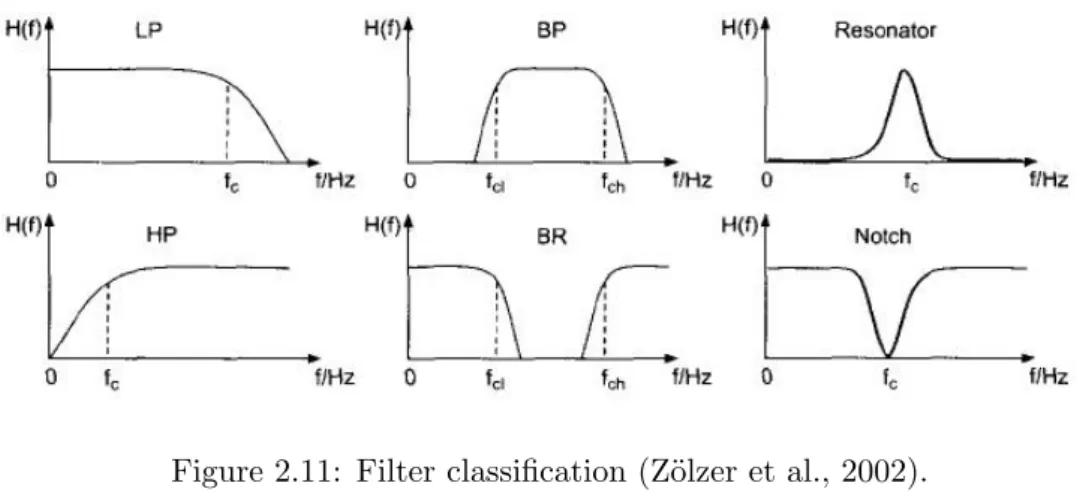
Figure 2.11: Filter classification (Z¨olzer et al., 2002).

• Subtract the average value of the function from each value and then divide by the maximum absolute deviation, so that the average will be 0 and the standard deviation 1 (later we will call this normalization method by stdev).

The filters used are typically low pass filters (Bello et al., 2005; Holzapfel et al., 2010; Dixon, 2006), which, in general, select low frequencies up to the cut-off frequency (fc) and

attenuate frequencies higher than fc(Z¨olzer et al., 2002) and can be defined as:

yi = αxi+ (1 − α)yi−1 (2.19)

With the smoothing factor α defined as:

α = ∆T

RC + ∆T (2.20)

where ∆T is the inverse of the sampling frequency and the cut-off frequency is:

fc=

1

2πRC (2.21)

2.2.3.2 Thresholding

Even after post-processing there will be certain peaks that do not correspond to onsets. So, it is common to define a threshold that separates event-related and non-event-related peaks (Bello et al., 2005).

(46)

The first approach is to define a constant threshold (Klapuri et al., 2006) (see Fig. 2.12), δ, and, in this case, onsets would be peaks where the detection function, d, is bigger than the threshold: d(n) ≥ δ (2.22) -0.1 0 0.1 0.2 0.3 0.4 0.5 0.6 0.7 0.8 0.9 1 0.5 1 1.5 2 2.5 3 3.5 Amplitude Time HFC constant threshold

Figure 2.12: Constant threshold.

Since music typically exhibits great dynamics, constant thresholds usually give weak re-sults (Bello et al., 2005), so it is common to use adaptive thresholds (Holzapfel et al., 2010; Dixon, 2006). An adaptive threshold can be constructed in several ways. An option is to make use of a linear LP-FIR filter (Holzapfel et al., 2010; Bello et al., 2005):

˜ δ = δ + M X i=0 aid(n − i) (2.23)

where ai are the filter coefficients. Other option is to use the square of the detection

(47)

2.2. ONSET DETECTION METHODS 25 ˜ δ = δ + λ M X i=−M wid2(n − i) (2.24)

where λ is a positive constant and wi is a smooth window of choice.

Although better than the constant threshold, the previous adaptive thresholds still present problems when facing musics with great dynamical change. The best way to overcome this problems is to build a function based on the local mean (see Fig 2.13) or local median of the detection function, d (Kauppinen, 2002):

˜

δ(n) = δ + λ mean(|d(n − M )|, ...., |d(n + M )|) (2.25)

or

˜

δ(n) = δ + λ median(|d(n − M )|, ...., |d(n + M )|) (2.26) where λ and δ are positive constants, that can be tweaked, and M is the size of a window around each of the points of the detection function.

These threshold functions based on the mean and on the median are the most robust to signal dynamics (Bello et al., 2005; Dixon, 2006; Kauppinen, 2002).

It is important to notice that the parameters used in thresholding have a large impact on the final results, mainly in the ratio of false positives to false negatives (Dixon, 2006).

2.2.3.3 Peak-picking

After the above procedures, picking the onsets, o(n), is reduced to the identification of local maxima above the defined threshold, which can be summarized as (Eyben et al., 2010):

o(n) =                        1 if d(n) > ˜δ(n) and d(n − w) ≤ d(n) ≤ d(n + w) 0 otherwise (2.27)

(48)

-0.2 0 0.2 0.4 0.6 0.8 1 0.5 1 1.5 2 2.5 3 3.5 Amplitude Time HFC running-mean threshold

Figure 2.13: Running-mean adaptive threshold.

2.3 Summary

In this chapter, we define the concept of onset, discussing the difficulties and ambiguities in the definition, and the concept of onset class, that is, the classification of onsets.

The complete process that leads from the audio signal to the onsets – pre-processing, reduction and peak selection – is explained and each step focused.

Pre-processing methods, in general, try to emphasize the features relevant to onset detec-tion, in order to help the subsequent stages.

When it comes to the Detection Function step of Onset Detection, it can be of several types. From the perspective of representation of the signal, the Onset Detection functions can be of Time Domain or Spectral Domain type; although, according to other properties, we have also other possibilities for classifying detection functions: probabilistic, pitch-based, and data-driven.

The spectral-domain OSS are the most focused on this chapter, as this is the type of functions created and explored in Chapter 3. The most common spectral-domain OSS are the

(49)

2.3. SUMMARY 27 High Frequency Function, the Spectral Flux, the Phase Deviation family and the Complex Domain family. The HFC, SF and PD use only information from the magnitude of the spectrum, while the Complex Domain family (CD and RCD functions) and the WPD function use information from both the magnitude and phase of the spectrum.

Next, we describe the Peak Selection step of onset detection, that is, how can one select the peaks of the OSS functions that correspond to onsets. This step usually consists of 3 parts: post-processing, thresholding and peak selection. The post-processing part is responsible for making the OSS more uniform, while the threshold – usually a dynamic and not a constant threshold – separate even-related from non-event-related peaks. Finally, the peak picking is responsible for collecting the position of the peaks that are greater than the threshold.

(50)

(51)

3

Analysis of Onset

Detection Performance

Aiming at providing the most complete possible information about Onset Detection, a selec-tion of six Onset Detecselec-tion Methods using Spectral Features, described in Chapter 2, were explored in this chapter using two approaches:

• Direct comparison of the performance of each Onset Detection Method;

• Assessment of the influence of the Peak Selection part of Onset Detection process on the results of each OSS.

In order to be able to follow these two approaches, one must define first how the results are evaluated – the evaluation metrics (Section 3.1) – and on which audio signals the methods will be tested – the datasets (Section 3.2).

3.1 Evaluation Metrics

When facing classification problems, the main source for performance measurements is called a Classification Matrix (Olson & Delen, 2008), and it can be defined as in Table 3.1.

True (Reference)

Predicted True Positive (TP) False Positive (FP) (Inferred) False Negative (FP) True Negative (TN)

Table 3.1: Classification Matrix

The upper-left to lower right diagonal of the matrix represent the correct decisions made while the other diagonal represent the errors made (Olson & Delen, 2008). With the help of this matrix, we can define several useful quantities, that are depicted in Fig. 3.1.

With the help of both the classification matrix (Table 3.1) and Fig. 3.1, it is possible to define Precision, Recall and F-measure, the quantities that will be used to evaluate the results in Section 3.3, Section 3.4 and Section 3.5.

(52)

FP

TN

Inferred

Reference

Figure 3.1: Relationship between the quantities defined in the Classification Matrix (Manning et al., 2008)

The Precision (also called overall accuracy (Olson & Delen, 2008)), that is, the fraction of retrieved instances that are relevant, is defined by dividing the total correctly detected positives by the total number of returned results.

P recision = T P

T P + F P (3.1)

On the other hand, the Recall (also called true positive rate or hit rate), that is, the fraction of relevant instances that are retrieved, is obtained by dividing the correctly detected positives by the number of results that should have been returned.

Recal = T P

T P + F N (3.2)

In the particular case of onset detection one can interpret the TP as the correctly detected onsets, the FP as falsely detected onsets and the FN as onsets that were not detected.

It is important to note that the Mirex Onset Detection Task specifications (MIREX, 2011), and most of the papers in this area, consider onsets detected as TP if they are in a window of 50ms around the annotated onset. On the other hand, if more than one detection fall inside the same tolerance window, only one is counted as TP, the others are considered as FP. When a detection is inside the tolerance window of two onset annotations, one TP and one FN are counted.

We can also define a quantity that joins both precision and recall in a sort of weighted average. It is called F-measure and can be obtained by:

(53)

3.2. DATASETS 31 F-measure = ₁ 2 P + 1 R = 2 · P · R P + R (3.3)

There is another form of evaluation, called Correct Detection Rate(CDR) (Liu et al., 2003; Collins, 2005a), defined as:

CDR = total − F N − F P

total (3.4)

3.2 Datasets

The main difficulty with evaluating an onset detection algorithm is that of having a signifi-cantly large balanced songs for which the onset times are known (Dixon, 2006). This is not easy to achieve, because precise onset times are available only to a small amount of musics, such as produced by computer-monitored pianos (Dixon, 2006), and all the other has to be labelled by hand, which is an error-prone task.

With these difficulties in mind, we chose to datasets: one publicly available, and the other developed for a paper by Bello et al. (2005).

3.2.1 Alicante Dataset

The Alicante Dataset is a publicly available annotated dataset (Alicante, 2012) created by the Pattern Recognition and Artificial Intelligence Group of the University of Alicante (PRAIg-UA). This dataset contains 19 real recordings that cover a relatively wide range of instruments and musical genres (Alicante, 2012) and 2155 onsets. The songs are available in WAV format (sample rate 22.050 kHz, mono, 16 bit) and their onset positions (in seconds) in text format. We can divide the recordings of the dataset in 3 distinct groups, according to the charac-teristic of their onsets: Complex Mixture (Mix), Pitched Non-percussive (PNP) and Pitched Percussive (PP), as show in Table 3.2.

The ground truth onset labelling in this dataset was marked and reviewed with the help of the software Speech Filling QSystem (Sciences, 2012).

(54)

No. Songs No. Onsets

Mix 11 1397

PNP 3 254

PP 5 504

Total 19 2155

Table 3.2: Alicante Dataset Structure 3.2.2 Bello Dataset

The Bello Dataset is a hand labelled and annotated dataset first proposed in Bello et al. (2005) and used in several other works, such as the ones of Dixon (2006) and Holzapfel et al. (2010). It contains commercial and non-commercial recordings, covering a variety of musical styles and instrumentations, in a total of 23 songs (Bello et al., 2005) and 1065 onsets. The songs are available in WAV format (sample rate 22.050 kHz, mono, 16 bit) and their onset positions (in seconds) in text format.

One can group the songs in this dataset just as it was done for the previous dataset, but adding the NPP class that was absent in the Alicante Dataset. This grouping of songs by onset classes is described in Table 3.3.

No. Songs No. Onsets

Mix 7 271

PNP 1 93

PP 9 489

NPP 6 212

Total 23 1065

Table 3.3: Bello Dataset Structure

3.3 Comparison of OSS functions Using Spectral

Fea-tures

In order to compare the performance of the different Onset Detection Methods, the algorithms of 6 Onset Detection Methods using Spectral Features were reproduced: HFC, SF, PD, WPD, CD, and RCD.

Several experiments were created to test and compare the behaviour of these Onset De-tection Methods according to the different Onset Classes and to the two datasets described

(55)

3.3. COMPARISON OF OSS FUNCTIONS USING SPECTRAL FEATURES 33 in the previous section.

3.3.1 Experiments

The following general steps were used to run the experiments:

• Read the data from the WAV file;

• Build the detection functions with the help of a spectral-domain representation of the signal obtained by the calculus of consecutive STFT (with Hamming-window size and hop size as parameters);

• Normalize the detection function so that it will be in the interval [-1, 1] and its average will be zero, that is, for each value one subtracts the mean and divides by the maximum value;

• Create a running-median threshold, as defined in Eq. 2.25, with λ, delta and M as parameters;

• Consider as onset every value in the detection function that is bigger than the threshold and is a local maximum (in a window of 3 samples around it).

We ran our experiments in the Alicante and Bello datasets by varying the parameters with the purpose of maximizing the F-measure for each group of onsets (Mix, PP, PNP and NPP) described in the previous subsection. By multiple experiments we found that the maximum values for F-measure appear when we use a window of 1024 samples (that is 46.4ms in this 22.05kHz sampled signals) with hop size of 50% when calculating the STFT and by setting M = 10 in Eq. 2.25. Moreover, we found that the best threshold parameters λ and δ varied per group of musics. Hence, the results presented and discussed in the next section were all obtained by varying the parameters λ and δ between 0 and 1, maintaining the other parameters fixed to the values stated.

(56)

F-measure Precision Recall HFC 0.708 0.724 0.692 SF 0.840 0.829 0.852 PD 0.455 0.390 0.557 WPD 0.704 0.693 0.715 CD 0.768 0.781 0.755 RCD 0.771 0.741 0.804

Table 3.4: Overal Results by OSS in the Alicante Dataset F-measure Precision Recall

HFC 0.781 0.760 0.806 SF 0.921 0.930 0.913 PD 0.589 0.465 0.816 WPD 0.794 0.780 0.813 CD 0.835 0.830 0.843 RCD 0.856 0.856 0.860

Table 3.5: Overal Results by OSS in the Bello Dataset

PP PNP Mix F P R F P R F P R HFC 0.814 0.849 0.801 0.542 0.555 0.529 0.783 0.784 0.782 SF 0.921 0.916 0.926 0.780 0.794 0.767 0.816 0.776 0.861 PD 0.377 0.281 0.668 0.473 0.423 0.534 0.529 0.468 0.610 WPD 0.825 0.822 0.843 0.606 0.612 0.600 0.804 0.791 0.816 CD 0.883 0.923 0.848 0.621 0.651 0.594 0.824 0.827 0.821 RCD 0.893 0.911 0.875 0.694 0.675 0.714 0.797 0.747 0.854

Table 3.6: Results for the Alicante Dataset: Precision(P), Recall(R), and F-measure(F)

NPP PP F P R F P R HFC 0.921 0.922 0.920 0.838 0.846 0.830 SF 0.931 0.946 0.926 0.961 0.964 0.947 PD 0.652 0.573 0.819 0.497 0.410 0.734 WPD 0.916 0.959 0.882 0.810 0.796 0.826 CD 0.947 0.978 0.923 0.883 0.892 0.874 RCD 0.933 0.977 0.903 0.882 0.880 0.883

Table 3.7: Results for NPP and PP onset classes in the Bello Dataset: Precision(P), Recall(R), and F-measure(F) PNP Mix F P R F P R HFC 0.553 0.519 0.591 0.812 0.753 0.881 SF 0.911 0.888 0.935 0.880 0.922 0.842 PD 0.615 0.479 0.860 0.540 0.396 0.851 WPD 0.660 0.602 0.731 0.832 0.762 0.811 CD 0.684 0.650 0.720 0.866 0.798 0.854 RCD 0.808 0.745 0.882 0.824 0.823 0.770

Table 3.8: Results for PNP and Mix onset classes in the Bello Dataset: Precision(P), Re-call(R), and F-measure(F)

(57)

3.3. COMPARISON OF OSS FUNCTIONS USING SPECTRAL FEATURES 35 3.3.2 Results & Discussion

The results of our experiments are shown in Table 3.4, to Table 3.8, and in Figures 3.2 and 3.3. These results were obtained by choosing the parameters that maximize the F-measure for each group of onsets.

The results in the two datasets allow us to notice right away that the PNP onset type has the lower performance, that is, soft onsets are harder to detect. This result is in complete agreement with the results in the literature (Bello et al., 2005; Dixon, 2006; Holzapfel et al., 2010). 0.65 0.7 0.75 0.8 0.85 0.9 0.95 1 0 0.1 0.2 0.3 0.4 0.5 0.6 0.7 0.8 0.9 1 Precision Recall SF - Mix SF - NPP SF - PP SF - PNP

Figure 3.2: Precision vs Recall for the SF OSS in all the onset classes of the Bello Dataset.

In general, the results are better for the NPP class (in the Bello Dataset), followed by the PP, Mix and lastly by the PNP class. Although there are some exceptions: the PD OSS performs best for the Mix onsets on the Alicante dataset and the in the Bello Dataset it performs worse for the PP class.

(58)

The organization of the tables allow us to understand easily how each detection function performs on the different onset classes.

Globally, when looking at the results, one can clearly see that the SF was the best overall performer – except for Mix onsets in the Alicante Dataset and NPP onsets in the Bello Dataset – followed closely by the CD, RCD and WPD functions, a result that confirms previously obtained results in the literature (Bello et al., 2005; Dixon, 2006). Also confirmed by previous literature (Dixon, 2006) is the PD as the function with the worst performance.

One can try to explain the overall poor results obtained with the PD detection function with the impact it suffers from the phase distortion of signals where percussive sounds have preponderance. Although this fact counts for explaining well the PD results in the PP and Mix onset types, it does not explain why the PD still performs badly for PNP onsets, where the phase distortion does not have a clear impact. A possible explanation to these poor results by the PD function is some sort of possible filter and/or normalization that the authors that proposed this method used but did not publish in their papers.

Our results show also, in accordance with Dixon (2006), that the WPD function brings great improvement on the results of the PD function. In the dataset used, for PP onset types, this improvement is of more than 30pp1. On the contrary, the improvements brought by the RCD function to the CD function are not as relevant and for the Mix onset class in both the datasets the RCD performs 3 to 4pp worse than the CD function.

As expected, the HFC presents very good results – staying very close to the results of the WPD, CD and RCD OSS – for Mix, PP and NPP onsets, that is, those onsets where the percussive components are predominant, lowering its performance for the PNP onsets. All in all, the HFC presents very high results in this two datasets, mainly because they are largely dominated by percussive onsets.

The functions that use information from the magnitude and phase of the spectrum per-form relatively well in al onset classes except the PNP, where the results drop most of the times by 20pp. The overall good performance of this functions is in aggreement with the liter-ature (Duxbury, Bello, Davies, & Sandler, 2003; Dixon, 2006; Bello et al., 2005), although the

1

(59)

3.3. COMPARISON OF OSS FUNCTIONS USING SPECTRAL FEATURES 37 0.65 0.7 0.75 0.8 0.85 0.9 0.95 1 0 0.1 0.2 0.3 0.4 0.5 0.6 0.7 0.8 0.9 1 Precision Recall RCD - Mix RCD - NPP RCD - PP RCD - PNP

Figure 3.3: Precision vs Recall for the RCD OSS in all the onset classes of the Bello Dataset.

drop of performance for the PNP class was not something to be expected a priori from the lit-erature. A possible explanation for this fact is some kind of problem with the implementation done of the algorithms proposed by the authors.

By comparing Table 3.4 with Table 3.5 and Table 3.6 with Tables 3.7 and 3.8, we can see that, in general, the results in the Bello Dataset outperform those in the Alicante Dataset. The only exceptions are the WPD, CD and RCD OSS which perform slightly better in the Alicante Dataset for the PP onset class.

A possible explanation for this result can be the fact that the Bello Dataset has more percussive onsets than the Alicante Dataset, being the percussive onsets – PP and NPP onset classes – easier to detect than the PNP and Mix onset classes.

On a song per song basis, the results allow us to understand that even between different songs with the same type of onsets, the results can be quite different. This fact can be used to explain the differences in performance between the two datasets, and means that the dataset

(60)

chosen can influence significantly the results.

It is not only the maximum values of F-measure for each detection function that one wants to analyse; the relation of false positives to true positives is also relevant, because it tells us information about the properties of the detection function. One can see the true positives vs false positives relationship by drawing a graph TP vs FP or by drawing a Precision vs Recall curve.

Figures 3.2 and 3.3 depict the precision vs recall curve of our results in the case of the SF and RCD detection functions for all onset classes in the Bello Dataset. The figures were obtain by varying δ in small steps.

The ideal case would be a curve touching the top-right corner (Precision = 1, Recall = 1) of a graphic of this type, that is, detecting all onsets without any false positives. That is something very hard to achieve, but one wants a curve as close to the top-right corner as possible.

Since some applications, like tempo estimation, require high accuracy on the detected onsets (that is, as few false positives as possible) even if missing a few onsets, and other ap-plications require the maximization of the percentage of detections, even if increasing number of FP, the behaviour of this curve is of great interest when choosing which onset detection function to use. This clearly means that the choice of onset detection function depends on the particular application where one wants to apply the onsets obtained.

3.4 Influence of interpretation style on Onset Detection

An interesting result that was not reported yet in the literature was obtained with the previous experiments.

In Tables 3.9 and 3.10, we show the top 5 results of two violin songs from the PNP class of the Alicante Dataset: the violin song 1 is a simple song played with the most common violin techniques, while the violin song 2 is a piece composed by the Italian composer Niccol`o Paganini and it requires several skilful and advanced techniques (like very fast arpeggios, and extreme glissando) in order to be performed correctly.

(61)

3.5. INFLUENCE OF PEAK SELECTION METHODS ON ONSET DETECTION 39 F-measure Precision Recall

SF 0.828 0.759 0.911

SF 0.825 0.769 0.888

SF 0.816 0.755 0.888

Table 3.9: Top 5 results for violin song 1 - common interpretation F-measure Precision Recall

CD 0.810 0.899 0.737

CD 0.806 0.888 0.737

CD 0.804 0.878 0.742

CD 0.803 0.868 0.747

Table 3.10: Top 5 results for violin song 2 - virtuoso interpretation

The F-measure results are similar in the two songs, although the OSS function that dominates the top results is not the same in the two cases. For the common interpretation, the SF function dominates, while for the virtuoso song, the CD achieves the top results. This means that the advanced violin technique produces softer onsets than the usual technique and that the CD is able to distinguish between closer onsets than the SF in this particular case. These results, however, cannot be generalized, as the dataset only has two songs of this type.

3.5 Influence of Peak Selection Methods on Onset

De-tection

Several papers in this area (Bello et al., 2005; Dixon, 2006; Holzapfel et al., 2010), mention that the Peak Selection part of the Onset Detection process influences greatly the final results. However, at the present time, to the best of our knowledge, there is no study that deeply explores this influence.

With this in mind, we tested the six Onset Detections developed and compared in Sec-tion 3.3 with five different Peak SelecSec-tion Methods in order to test and compare the influence of four different aspects of Peak Selection:

(62)

• Normalization type;

• The use of a smoothing filter;

• The use of a local maximum for selecting peaks.

3.5.1 Experiments

In order to assess the influence of peak selection methods on the results of onset detection, different simulations were run each with a particular peak selection method. These methods were selected because they have been used in recent work (Bello et al., 2005; Dixon, 2006; Holzapfel et al., 2010).

We used the following abbreviations to name the used peak selection methods:

norm Normalize the detection function by dividing by the absolute maximum and subtract-ing the average value, so that the average will be zero.

stdev Normalize the detection function by dividing by the maximum standard deviation and subtracting the average value, so that the average will be zero.

mean Create a running mean threshold (Eq. 2.26). median Create a running median threshold (Eq. 2.25).

filter Before normalization, smooth the detection function by applying a simple low pass filter (Eq. 2.19).

no-filter Do not apply the low pass filter, that is, do not use smoothing.

local-max Consider as onsets every value in the detection function that is greater than zero, greater than the threshold and is a local maximum in a window of 3 samples around it. I.e., use w = 3 in Eq. 2.27.

no-local-max Consider as onset every value bigger than the threshold. In other words, use w = 0 in Eq. 2.27.

(63)

3.5. INFLUENCE OF PEAK SELECTION METHODS ON ONSET DETECTION 41 A B C D E norm × × × × stdev × mean × median × × × × filter × local-max × × × ×

Table 3.11: Components of the Peak Selection Methods A, B, C, D and E.

First we run our experiments with the peak selection method median-norm-no-filter-local-max(A), then we replaced the running mean threshold with a running average-threshold with parameter M = 10 by running the experiments with the peak selection method mean-norm-no-filter-local-max(B).

After that, in order to assess the influence of the type of normalization, we ran the experiments by replacing the norm type of normalization with the stdev type of normalization, that is, using the peak selection method median-stdev-no-filter-local-max(C).

We also tested the influence of a smoothing step before the peak selection – with the use of a simple lp-filter – by running the experiments with the median-norm-filter-local-max(D) peak selection method.

Finally, to test the final peak picking algorithm’s influence, we ran the experiments without the local maximum condition, that is we used the median-norm-no-filter-no-local-max(E) peak selection method.

3.5.2 Results & Discussion

A B C F P R F P R F P R HFC 0.921 0.922 0.920 0.922 0.957 0.901 0.921 0.922 0.920 SF 0.931 0.946 0.926 0.943 0.957 0.937 0.934 0.946 0.932 PD 0.652 0.573 0.819 0.650 0.571 0.819 0.652 0.573 0.819 WPD 0.916 0.959 0.882 0.922 0.933 0.918 0.914 0.945 0.891 CD 0.947 0.978 0.923 0.946 0.987 0.913 0.943 0.970 0.923 RCD 0.933 0.977 0.903 0.933 0.966 0.913 0.936 0.977 0.908

Table 3.12: Results for NPP onsets in the Bello Dataset using the Peak Selection methods A, B, and C: P, Precision, F, F-measure and R, Recall.

(64)

D E F P R F P R HFC 0.823 0.913 0.766 0.622 0.525 0.798 SF 0.939 0.953 0.933 0.782 0.709 0.903 PD 0.628 0.586 0.749 0.520 0.417 0.893 WPD 0.828 0.900 0.778 0.603 0.507 0.816 CD 0.872 0.931 0.835 0.583 0.482 0.820 RCD 0.909 0.919 0.904 0.419 0.298 0.824

Table 3.13: Results for NPP onsets in the Bello Dataset using the Peak Selection methods D and E: P, Precision, F, F-measure and R, Recall.

A B C F P R F P R F P R HFC 0.838 0.846 0.830 0.848 0.829 0.867 0.842 0.846 0.839 SF 0.961 0.968 0.954 0.965 0.978 0.953 0.961 0.969 0.954 PD 0.497 0.410 0.734 0.488 0.414 0.740 0.388 0.278 0.823 WPD 0.810 0.796 0.826 0.811 0.793 0.830 0.811 0.793 0.830 CD 0.883 0.892 0.874 0.899 0.876 0.923 0.903 0.883 0.923 RCD 0.882 0.880 0.883 0.891 0.863 0.920 0.881 0.823 0.947

Table 3.14: Results for PP onsets in the Bello Dataset using the Peak Selection methods A, B, and C: P, Precision, F, F-measure and R, Recall.

size of the STFT at 1024 samples (that is 46.4ms in these 22.05kHz sampled signals) with hop size of 50%. The parameters δ and λ are tweaked while running the experiments, in order to obtain the values that maximize the f-measure.

The results obtained by running the experiments in the Bello dataset with all the peak selection methods described in the previous section are shown in Tables 3.12 through 3.19.

In order to do the comparisons, we consider as base the results with the peak selection method A and compare all others with this one.

First we will analyse the influence of the peak selection methods on the results obtained for the different onset classes and next we will analyse the influence of the peak selection methods on each of the OSS, and, finally, we will make a global balance about the significance of the compared results of the different Peak Selection Methods.

3.5.2.1 Onset Classes

The differences between running the experiments by using a running-median threshold – Peak Selection Method A – or a running-mean threshold – Peak Selection Method B – have mixed behaviours according to the onset classes. In the NPP and PP classes, the mean gives slightly

Onset detection in music signals

Onset Detection in Music Signals

Onset Detection in Music Signals

Resumo

Abstract

Palavras Chave

Keywords

Palavras Chave

Keywords

Acknowledgements

“Music is a moral law. It gives soul to the universe, wings to the mind,

flight to the imagination, and charm and gaiety to life and to

everything”

Plato

Contents

List of Figures

List of Tables

1

Introduction

1.1

Context & Motivation

1.2

Objectives

1.3

Thesis Contributions

1.4

Related Publications

1.5

Outline of the Thesis

2

Onset Detection

2.1

Definitions

2.2

Onset Detection Methods

2.3

Summary

3

Analysis of Onset

Detection Performance

3.1

Evaluation Metrics

FP

TN

Inferred

Reference

3.2

Datasets

3.3

Comparison of OSS functions Using Spectral

Fea-tures

3.4

Influence of interpretation style on Onset Detection

3.5

Influence of Peak Selection Methods on Onset

De-tection