Emotionally-Relevant Features for Classification and Regression of Music Lyrics

Emotionally-Relevant Features for Classification

and Regression of Music Lyrics

Ricardo Malheiro, Renato Panda, Paulo Gomes and Rui Pedro Paiva

Abstract— This research addresses the role of lyrics in the music emotion recognition process. Our approach is based on several state of the art features complemented by novel stylistic, structural and semantic features. To evaluate our approach, we created a ground truth dataset containing 180 song lyrics, according to Russell’s emotion model. We conduct four types of experiments: regression and classification by quadrant, arousal and valence categories. Comparing to the state of the art features (ngrams - baseline), adding other features, including novel features, improved the F-measure from 69.9%, 82.7% and 85.6% to 80.1%, 88.3% and 90%, respectively for the three classification experiments. To study the relation between features and emotions (quadrants) we performed experiments to identify the best features that allow to describe and discriminate each quadrant. To further validate these experiments, we built a validation set comprising 771 lyrics extracted from the AllMusic platform, having achieved 73.6% F-measure in the classification by quadrants. We also conducted experiments to identify interpretable rules that show the relation between features and emotions and the relation among features. Regarding regression, results show that, comparing to similar studies for audio, we achieve a similar performance for arousal and a much better performance for valence.

Index Terms—affective computing, affective computing applications, music retrieval and generation, natural language processing, recognition of group emotion

——————————  ——————————

1

I

usic emotion recognition (MER) is gaining significant at-tention in the Music Information Retrieval (MIR) scientific community. In fact, the search of music through emotions is one of the main criteria utilized by users [1].

Real-world music databases from sites like AllMusic1 _or

Last.fm2 _{grow larger and larger on a daily basis, which requires}

a tremendous amount of manual work for keeping them up-dated. Unfortunately, manually annotating music with emotion tags is normally a subjective process and an expensive and time-consuming task. This should be overcome with the use of auto-matic recognition systems [2].

Most of the early-stage automatic MER systems were based on audio content analysis (e.g., [3]). Later on, researchers started combining audio and lyrics, leading to bi-modal MER systems with improved accuracy (e.g., [2], [4] [5]). This does not come as a surprise since it is evident that the importance of each dimen-sion (audio or lyrics) depends on music style. For example, in dance music audio is the most relevant dimension, while in po-etic music (like Jacques Brel) lyrics are key.

Several psychological studies confirm the importance of lyr-ics to convey semantical information. Namely, according to Juslin and Laukka [6], 29% of people mention that lyrics are an important factor of how music expresses emotions. Also, Besson et al. [7] have shown that part of the semantic information of songs resides exclusively in the lyrics.

Despite the recognized importance of lyrics, current research in Lyrics-based MER (LMER) is facing the so-called glass-ceiling

1 _{AllMusic - http://www.allmusic.com/}

[8] effect (which also happened in audio). In our view, this ceil-ing can be broken with recourse to dedicated emotion-related lyrical features. In fact, so far most of the employed features are directly imported from general text mining tasks, e.g., bag-of-words (BOW) and part-of-speech (POS) tags, and, thus, are not specialized to the emotion recognition context. Namely, these state-of-the-art features do not account for specific text emotion attributes, e.g., how formal or informal the text language is, how the lyric is structured and so forth.

To fill this gap we propose novel features, namely:

 Slang presence, which counts the number of slang words from a dictionary of 17700 words;

 Structural analysis features, e.g., the number of repeti-tions of the title and chorus, the relative position of verses and chorus in the lyric;

 Semantic features, e.g., gazetteers personalized to the employed emotion categories.

Additionally, we create a new, manually annotated, (par-tially) public dataset to validate the proposed features. This might be relevant for future system benchmarking, since none of the current datasets in the literature is public (e.g., [5]). More-over, to the best of our knowledge, there are no emotion lyrics datasets in the English language that are annotated with contin-uous arousal and valence values.

The paper is organized as follows. In section 2, the related work is described and discussed. Section 3 presents the methods employed in this work, particularly the proposed features and ground truth. The results attained by our system are presented and discussed in Section 4. Finally, section 5 summarizes the main conclusions of this work and possible directions for future research.

2 _{Last.fm - http://www.lastfm.pt/}

xxxx-xxxx/0x/$xx.00 © 200x IEEE Published by the IEEE Computer Society

M

————————————————

 R. Malheiro is with Center for Informatics and Systems of the University of Coimbra (CISUC) and Miguel Torga Higher Institute. E-mail: rsmal@ dei.uc.pt.

2

R

W

The relations between emotions and music have been a subject of active research in music psychology for many years. Different emotion paradigms (e.g., categorical or dimensional) and taxon-omies (e.g., Hevner, Russell) have been defined [9], [10] and ex-ploited in different computational MER systems.

Identification of musical emotions from lyrics is still in an em-bryonic stage. Most of the previous studies related to this subject used general text instead of lyrics, polarity detection instead of emotion detection. More recently, LMER has gained significant attention by the MIR scientific community.

Feature extraction is one of the key stages of the LMER pro-cess. Previous works employing lyrics as a dimension for MER typically resort to content-based features (CBF) like Bag-Of-Words (BOW) [5], [11], [12] with possible transformations like stemming and stopwords removal. Other regularly used CBFs are Part-Of-Speech (POS) followed by BOW [12]. Additionally, linguistic and text stylistic features [2], are also employed.

Despite the relevance of such features and their possibility of use in general contexts, we believe they do not capture several aspects that are specific of emotion recognition in lyrics. There-fore, we propose new features, as will be described in Section 3.

As for ground truth construction, different authors typically construct their own datasets, annotating the datasets either man-ually (e.g., [11]), or acquiring annotated data from sites such as AllMusic or Last.fm (e.g., [12], [13]).

As for systems based on manual annotations, it is difficult to compare them, since they all use different emotion taxonomies and datasets. Moreover, the employed datasets are not public. As for automatic approaches, frameworks like AllMusic or Last.fm are often employed. However, the quality of these an-notations might be questionable because, for example in Last.fm, the tags are assigned by online users, which in some cases may cause ambiguity. In AllMusic, despite the fact that the annotations are made by experts [14], it is not clear whether they are annotating songs using only audio, lyrics or a combination of both.

Due to the limitations of the annotations in approaches like AllMusic and Last.fm and the fact that the datasets proposed by other researchers are not public, we decided to construct a man-ually annotated dataset. Our goal is to study the importance of each feature to the lyrics in a context of emotion recognition. So, the annotators have been told explicitely to ignore the audio during the annotations to measure the impact of the lyrics in the emotions. In the same way some researchers of the audio’s area ask annotators to ignore lyrics, when they want to evaluate models focused on audio [15]. This all independently of in the process of audition we may use both dimensions. In the future we intend to fuse both dimensions and make a bimodal analysis. Additionally, to facilitate future benchmarking, the constructed dataset will be made partially public3_{, i.e., we provide the names}

of the artists and the song titles, as well as valence and arousal values, but not the song lyrics, due to copyright issues; instead we provide the URLs from where each lyric was retrieved.

Most current LMER approaches are black-box models instead of interpretable models. In [14], the authors use a human-com-prehensible model to find out relations between features from General Inquirer (GI) and emotions. We use interpretable rules to match emotions and features not only from GI but from other

3 _{http://mir.dei.uc.pt/resources/MER_lyrics_dataset.zip}

types (e.g. Stylistic, Structural and Semantic) and platforms such as LIWC, ConcepNet and Synesketch.

3

M

3.1 Dataset Construction

As abovementioned, current MER systems either follow the categorical or the dimensional emotion paradigm. It is often ar-gued that dimensional paradigms lead to lower ambiguity, since instead of having a discrete set of emotion adjectives, emotions are regarded as a continuum [11]. One of the most well-known dimensional models is Russell’s circumplex model [16], where emotions are positioned in a two-dimensional plane comprising two axes, designated as valence and arousal, as illustrated in Figure 1. According to Russell [17], valence and arousal are the “core processes” of affect, forming the raw material or primitive of emotional experience.

Figure 1. Russell’s circumplex model (adapted from [11]).

3.1.1 Data Collection

To construct our ground truth, we started by collecting 200 song lyrics. The criteria for selecting the songs were the following:

 Several musical genres and eras (see Table 1);

 Songs distributed uniformly by the 4 quadrants of the Russell emotion model;

 Each song belonging predominantly to one of the 4 quadrants in the Russell plane.

To this end, before performing the annotation study de-scribed in the next section, the songs were pre-annotated by our team and were nearly balanced across quadrants.

Next, we used the Google API to search for the song lyrics. In this process, three sites were used for lyrical information: lyr-ics.com, ChartLyrics and MaxiLyrics.

The obtained lyrics were then preprocessed to improve their quality. Namely, we performed the following tasks:

 Correction of orthographic errors;

 Elimination of songs with non-English lyrics;

 Elimination of songs with lyrics with less than 100 char-acters;

 Elimination of text not related with the lyric (e.g., names of the artists, composers, instruments).

 Elimination of common patterns in lyrics such as [Cho-rus x2], [Vers1 x2], etc;

added to the lyrics).

To further validate our system, we have also built a larger validation set. This dataset was built in the following way:

1. First, we mapped the mood tags from AllMusic into the words from the ANEW dictionary (ANEW has 1034 words with values for arousal (A) and valence (V)). De-pending on the values of A and V, we can associate each word to a single Russell's quadrant. So, from that map-ping, we obtained 33 words for quadrant 1 (e.g., fun, happy, triumphant), 29 words for quadrant 2 (e.g., tense, nervous, hostile), 12 words for quadrant 3 (e.g., lonely, sad, dark) and 18 words for quadrant 4 (e.g., relaxed, gentle, quiet).

2. Then, we considered that a song belongs to a specific quadrant if all of the corresponding AllMusic tags belong to this quadrant. Based on this requirement, we initially extracted 400 lyrics from each quadrant (the ones with a higher number of emotion tags), using the AllMusic's web service.

3. Next, we developed tools to automatically search for the lyrics files of the previous songs. We used 3 sites: Lyr-ics.com, ChartLyrics and MaxiLyrics.

4. Finally, this initial set was validated by three people. Here, we followed the same procedure employed by Laurier [5]: a song is validated into a specific quadrant if at least one of the annotators agreed with AllMusic's an-notation (Last.FM in his case). This resulted into a dataset with 771 lyrics (211 for Q1, 205 for Q2, 205 for Q3, 150 for Q4). Even though the number of lyrics in Q4 is smaller, the dataset is still nearly balanced.

3.1.2 Annotations and Validation

The annotation of the dataset was performed by 39 people with different backgrounds. To better understand their background, we delivered a questionnaire, which was answered by 62% of the volunteers. 24% of the annotators who answered the ques-tionnaire have musical training and, regarding their education level, 35% have a BSc degree, 43% have an MSc, 18% a PhD and 4% have no higher-education degree. Regarding gender bal-ance, 60% were male and 40% were female subjects.

During the process, we recommended the following annota-tion methodology:

1. Read the lyric;

2. Identify the basic predominant emotion expressed by the lyric (if the user thought that there was more than one emotion, he/she should pick the predominant); 3. Assign values (between -4 and 4) to valence and

arousal; the granularity of the annotation is the unit, which means that annotators could use 9 possible val-ues to annotate the lyrics, from -4 to 4;

4. Fine tune the values assigned in 3) through ranking of the samples.

To further improve the quality of the annotations, the users were also recommended not to search for information about the lyric neither the song on the Internet or another place and to avoid tiredness by taking a break and continuing later.

We obtained an average of 8 annotations per lyric. Then, the arousal and valence of each song were obtained by the average of the annotations of all the subjects. In this case we considered

the average trimmed by 10% to reduce the effect of outliers. To improve the consistency of the ground truth, the standard deviation (SD) of the annotations made by different subjects for the same song was evaluated. Songs with an SD above 1.2 were excluded from the original set. As a result, 20 songs were dis-carded, leading to a final dataset containing 180 lyrics. This leads to a 95% confidence interval [18] of about ±0.4. We believe this is acceptable in our -4.0 to 4.0 annotation range. Finally the con-sistency of the ground truth was evaluated using Krippendorff’s alpha [19], a measure of inter-coder agreement. This measure achieved, in the range -4 up to 4, 0.87 and 0.82 respectively for the dimensions valence and arousal. This is considered a strong agreement among the annotators.

One important issue to consider is how familiar are the lyrics to the listeners. 13% of the respondents reported that they were familiar with 12% of the lyrics (on average). Nevertheless, it seems that the annotation process was sufficiently robust re-garding the familiarity issue, since there was an average of 8 an-notations per lyric and the annotation agreement (Krippen-dorff’s alpha) was very high (as discussed in the following chap-ters). This suggests that the results were not skewed.

Although the size of the dataset is not large, we think that is acceptable for experiments and is similar to other datasets man-ually annotated (e.g., [11] has 195 songs).

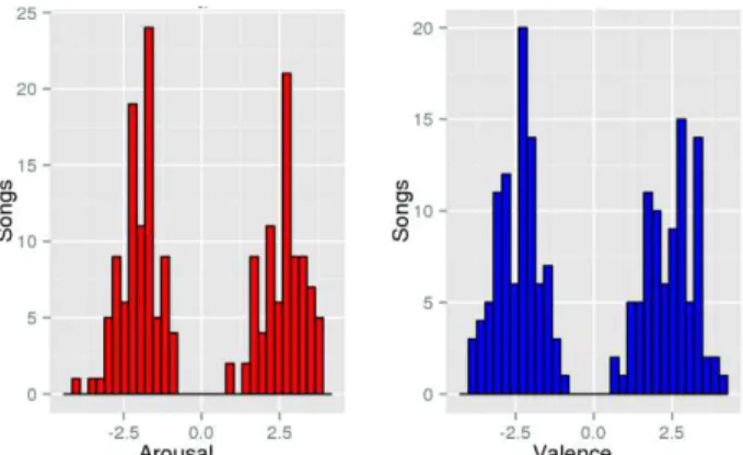
Figures 2 and 3 show the histogram for arousal and valence dimensions as well as the distribution of the 180 selected songs for the 4 quadrants.

Figure 2. Arousal and valence histogram values.

Figure 3. Distribution of the songs for the 4 quadrants.

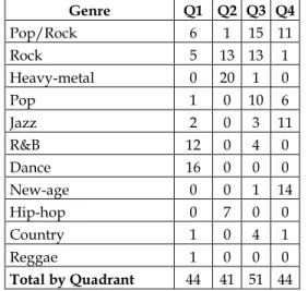
Table 1. Distribution of lyrics across quadrants and genres.

Genre Q1 Q2 Q3 Q4 Pop/Rock 6 1 15 11

Rock 5 13 13 1

Heavy-metal 0 20 1 0

Pop 1 0 10 6

Jazz 2 0 3 11

R&B 12 0 4 0

Dance 16 0 0 0

New-age 0 0 1 14

Hip-hop 0 7 0 0

Country 1 0 4 1

Reggae 1 0 0 0

Total by Quadrant 44 41 51 44

3.1.3 Emotion Categories

Finally, each song is labeled as belonging to one of the four pos-sible quadrants, as well as the respective arousal hemisphere (north or south) and valence meridian (east or west). In this work, we evaluate the classification capabilities of our system in the three described problems.

According to quadrants, the songs are distributed in the fol-lowing way: quadrant 1 – 44 lyrics; quadrant 2 – 41 lyrics; quad-rant 3 – 51 lyrics; quadrant 4 – 44 lyrics (see Table 1).

As for arousal hemispheres, we ended up with 85 lyrics with positive arousal and 95 with negative arousal.

Regarding valence meridian we have 88 lyrics with positive valence positive and 92 with negative valence.

3.2 Feature Extraction

3.2.1 Content-Based Features (CBF)

The most commonly used features in text analysis, as well as in lyric analysis, are content-based features (CBF), namely the bag-of-words (BOW) [20].

In this model the text in question is represented as a set of bags which normally correspond, in most cases, to unigrams, bi-grams or tribi-grams. The BOW are normally associated to a set of transformations such as stemming and stopwords removal which are applied immediately after the tokenization of the original text. Stemming allows each word to be reduced to its stem and it is assumed that there are no differences, from the semantic point of view, in words which share the same stem. Through stemming the words “argue”, “argued”, “argues”, “ ar-guing” e “argus” would be reduced to the same stem “argu”. The stopwords (e.g., the, is, in, at) which may also be called as function words are very common words in a certain language. These words bring normally little knowledge. The words in-clude mainly determiners, pronouns and other gramatical par-ticles which, by their frequency in a large quantity of docu-ments, are not discriminative. The BOW may also be applied without any of the prior transformations. This technique was used, for example, in [12].

Part-of-speech (POS) tags are another type of state-of-art fea-tures. They consist in attributing a corresponding grammatical class to each word. For example the grammatical tagging of the following sentence “The student read the book” would be

4 _{http://onlineslangdictionary.com/}

“The/DT student/NN read/VBZ the/DT book/NN”, where DT, NN and VBZ mean respectively determiner, noun and verb in 3rd person singular present. The POS tagging is typically fol-lowed by a BOW analysis. This technique was used in studies such as [21].

In our research we use all the combinations of unigrams, bi-grams, trigrams with the aforementioned transformations. We also use n-grams of POS tags from bigram to 5-grams.

3.2.2 Stylistic-Based Features (StyBF)

These features are related to stylistic aspects of the language. One of the issues related to the written style is the choice of the type of the words to convey a certain idea (or emotion, in our study). Concerning music, those issues can be related to the style of the composer, the musical genre or the emotions that we in-tend to convey.

We use 36 features representing the number of occurrences of 36 different grammatical classes in the lyrics. We use the POS tags in the Penn Treebank Project [22] such as for instance JJ (ad-jectives), NNS (noum plural), RB (adverb), UH (interjection), VB (verb). Some of these features are also used by authors like [12]. We use two features related to the use of capital letters: All Capital Letters (ACL), which represents the number of words with all letters in uppercase and First Capital Letter (FCL), which represents the number of words initialized by an uppercase let-ter, excluding the first word of each line.

Finally, we propose a new feature: the number of occurrences of slang words (abbreviated as #Slang). These slang words (17700 words) are taken from the Online Slang Dictionary4

(American, English and Urban Slang). We propose this feature because, in specific genres like hip-hop, the ideas are expressed normally with a lot of slang, so we believe that this feature may be important to describe specific emotions associated to specific genres.

3.2.3 Song-Structure-Based Features (StruBF)

To the best of our knowledge, no previous work on LMER em-ploys features related to the structure of the lyric. However, we believe this type of features has relevance for LMER. Hence, we propose novel features of this kind, namely:

 #CH, which stands for the number of times the chorus is repeated in the lyric;

 #Title, which is the number of times the title appears in the lyric.

 10 features based on the lyrical structure in verses (V) and chorus (C):

o _{#VorC (total of sections - verses and chorus - in the} lyrics);

o _{#V (number of verses);}

o _{C... (the lyric starts with chorus} – _boolean); o _{#V/Total (relation between Vs and the total of}

sec-tions);

o _{#C/Total (relation between C and the total of} sec-tions);

o _{>2CAtTheEnd (lyric ends with at least two} repeti-tions of the chorus – boolean);

chorus), VVCVC (between 2 chorus we have at least 1 verse).

Common sense says, for example, that normally more dance-able songs have more repetitions of the chorus. We believe that the different structures that a lyric may have, are taken into ac-count by the composers to express emotions. That is the reason why we propose these features.

3.2.4 Semantic-Based Features (SemBF)

These features are related to semantic aspects of the lyrics. In this case, we used features based on existing frameworks like Synesketch5 _{(8 features), ConceptNet}6 _{(8 features), LIWC}7 ₍₈₂

features) and GI8 _{(182 features).}

In addition to the previous frameworks, we use features based on known dictionaries: DAL [23] and ANEW [24]. From DAL (Dictionary of Affect in Language) we extract 3 features which are the average in lyrics of the dimensions pleasantness, activation and imagery. Each word in DAL is annotated with these 3 dimensions. As for ANEW (Affective Norms for English Words) we extract 3 features which are the average in lyrics of the dimensions valence, arousal and dominance. Each word in ANEW is annotated with these 3 dimensions.

Additionally, we propose 14 new features based on gazet-teers, which represent the 4 quadrants of the Russell emotion model. We constructed the gazetteers according to the following procedure:

1. We define as seed words the 18 emotion terms defined in Russell’s plane (see figure 1 in the article).

2. From the 18 terms, we consider for the gazetteers only the ones present in the DAL or the ANEW dictionaries. In DAL, we assume that pleasantness corresponds to va-lence, and activation to arousal, based on [25]. We em-ploy the scale defined in Dal: arousal and valence (AV) values from 1 to 3. If the words are not in the DAL dic-tionary but are present in ANEW, we still consider the words and convert the arousal and valence values from the ANEW scale to the DAL scale.

3. We then extend the seed words through Wordnet Affect [26], where we collect the emotional synonyms of the seed words (e.g., some synonyms of joy are exuberance, happiness, bonheur and gladness). The process of assign-ing the AV values from DAL (or ANEW) to these new words is performed as described in step 2.

4. Finally, we search for synonyms of the gazetteer’s cur-rent words in Wordnet and we repeat the process de-scribed in step 2.

Before the insertion of any word in the gazetteer (from step 1 on), each new proposed word is validated or not by two persons, according to its emotional value. There should be unanimity be-tween the two annotators. The two persons involved in the val-idation were not linguistic scholars but were sufficiently knowl-edgeable for the task.

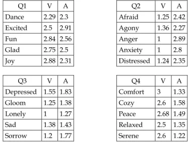
Table 2 illustrates some of the words for each quadrant.

5 _{http://synesketch.krcadinac.com/blog/} 6 _{http://web.media.mit.edu/~hugo/conceptnet/}

Table 2. Examples of words from the gazetteers in each quad-rant.

Q1 V A Q2 V A

Dance 2.29 2.3 Afraid 1.25 2.42 Excited 2.5 2.91 Agony 1.36 2.27 Fun 2.84 2.56 Anger 1 2.89 Glad 2.75 2.5 Anxiety 1 2.8 Joy 2.88 2.31 Distressed 1.24 2.35

Q3 V A Q4 V A

Depressed 1.55 1.83 Comfort 3 1.33 Gloom 1.25 1.38 Cozy 2.6 1.58 Lonely 1 1.27 Peace 2.68 1.49 Sad 1.38 1.43 Relaxed 2.5 1.35 Sorrow 1.2 1.77 Serene 2.6 1.22

Overall, the resulting gazeteers comprised 132, 214, 78 and 93 words respectively for the quadrants 1, 2, 3 and 4.

The features extracted are:

 VinGAZQ1 (average valence of the words present in the lyrics that are also present in the gazetteer of the quad-rant 1);

 AinGAZQ1 (average arousal of the words present in the lyrics that are also present in the gazetteer of the quad-rant 1);

 VinGAZQ2 (average valence of the words present in the lyrics that are also present in the gazetteer of the quad-rant 2);

 AinGAZQ2 (average arousal of the words present in the lyrics that are also present in the gazetteer of the quad-rant 2);

 VinGAZQ3 (average valence of the words present in the lyrics that are also present in the gazetteer of the quad-rant 3);

 AinGAZQ3 (average arousal of the words present in the lyrics that are also present in the gazetteer of the quad-rant 3);

 VinGAZQ4 (average valence of the words present in the lyrics that are also present in the gazetteer of the quad-rant 4);

 AinGAZQ4 (average arousal of the words present in the lyrics that are also present in the gazetteer of the quad-rant 4);

 #GAZQ1 (number of words of the gazetteer 1 that are present in the lyrics);

 #GAZQ2 (number of words of the gazetteer 2 that are present in the lyrics);

 #GAZQ3 (number of words of the gazetteer 3 that are present in the lyrics);

 #GAZQ4 (number of words of the gazetteer 4 that are present in the lyrics);

 VinGAZQ1Q2Q3Q4 (average valence of the words pre-sent in the lyrics that are also prepre-sent in the gazetteers of the quadrants 1, 2, 3, 4);

 AinGAZQ1Q2Q3Q4 (average arousal of the words pre-sent in the lyrics that are also prepre-sent in the gazetteers

7 _{http://www.liwc.net/}

of the quadrants 1, 2, 3, 4).

3.2.5 Feature grouping

The proposed features are organized into four different feature sets:

CBF. We define 10 feature sets of this type: 6 are BOW (1-gram up to 3-(1-grams) after tokenization with and without stem-ming (st) and stopwords removal (sw); 4 are BOW (2-grams up to 5-grams) after the application of a POS tagger without st and sw. These BOW features are used as the baseline, since they are a reference in most studies [2], [27].

StyBF. We define 2 feature sets: the first corresponds to the number of occurrences of POS tags in the lyrics after the appli-cation of a POS tagger (a total of 36 different grammatical classes or tags); the second represents the number of slang words (#Slang) and the features related to words in capital letters (ACL and FCL).

StruBF. We define one feature set with all the structural fea-tures.

SemBF. We define 4 feature sets: the first with the features from Synesketch and ConceptNet; the second with the features from LIWC; the third with the features from GI; and the last with the features from gazetteers, DAL and ANEW.

We use the term frequency and the term frequency inverse document frequency (tfidf) as representation values in the da-tasets.

3.3 Classification and Regression

For classification and regression, we use Support Vector Ma-chines (SVM) [28], since, based on previous evaluations, this technique performed generally better than other methods. A polynomial kernel was employed and a grid parameter search was performed to tune the parameters of the algorithm. Feature selection and ranking with the ReliefF algorithm [29] were also performed in each feature set, in order to reduce the number of features. In addition, for the best features in each model, we an-alyzed the resulting feature probability density functions (pdf) to validate the feature selection that resulted from ReliefF, as de-scribed below.

For both classification and regression, results were validated with repeated stratified 10-fold cross validation [30] (with 10 repetitions) and the average obtained performance is reported. Since we performed a very high number of experiments and each task uses different settings, it is not possible to present the employed parameters. We present, as an example, only the pa-rameters for the validation dataset (771 lyrics) in section 4.2.1.

4

R

D

4.1 Regression Analysis

The regressors for arousal and valence were applied using the feature sets for the different types of features (e.g., SemBF). Then, after feature selection, ranking and reduction with the Re-liefF algorithm, we created regressors for the combinations of the best feature sets.

To evaluate the performance of the regressors the coefficient of determination R2[31] was applied. This is a statistic that gives information about the goodness of fit of a model. This measure indicates how well data fit a statistic model. If value is 1, the model perfectly fits the data. A negative value indicates that the model does not fit the data at all.

Suppose a dataset with n values marked as

y

...

y

y

f

...

f

f

y

2

R is calculated as in (1).













  



i i i

i i

y y

f y

R ₂

2

2

1 (1)

2

R was computed separately for each dimension (arousal and valence).

The results were 0.59 (with 234 features) for arousal and 0.61 (with 340 features) for valence. The best results were achieved always with RBFKernel [32].

Yang [11] made an analogous study using a dataset with 195 songs (using only the audio). He achieved aR2score of 0.58 for arousal and 0.28 for valence. We can see that we obtained almost the same results for arousal (0.59 vs 0.58) and much better results for valence (0.61 vs 0.28). Although direct comparison is not pos-sible, these results suggest that lyrics analysis is likely to im-prove audio-only valence estimation. Thus, in the near future, we will evaluate a bi-modal analysis using both audio and lyrics. In addition, we used the obtained arousal and valence regres-sors to perform regression-based classification (discussed be-low).

4.2 Classification Analysis

We conduct three types of experiments for each of the defined feature sets: i) classification by quadrant categories; ii) classifica-tion by arousal hemispheres; iii) and classificaclassifica-tion by valence meridians.

4.2.1 Classification By Quadrant Emotion Categories

We can see in the following table (see Table 3) the performance of the best models for each one of the features categories (e.g., CBF). For CBF, we considered for example the two best models (M11 and M12). The field #Features-SelFeatures-FMeasure(%) represents respectively the total of features, the number of se-lected features and the results accomplished via the F-measure metric after feature selection.

Table 3. Classification by Quadrants: Best F-measure results for model.

Model ID Description

#Features- SelFeatures-FMeasure(%)

M11(CBF) BOW (unigrams) 3567-200-70.1

M12(CBF) POS+BOW(trigrams) 4687-700-64.5

M21(StyBF) #POS_Tags 34-20-51

M22(StyBF) #Slang+ACL+FCL 3-3-36.7

M31(StruBF) Structural Lyric Features 12-11-34.7

M41(SemBF) LIWC 82-39-71.1

M42(SemBF) Features based on gazeteers 20-20-65.3

M43(SemBF) GI 182-90-61.7

In the table above, M1x stands for models that employ CBF features, M2x represents models with StyBF features, M3x StruBF features and M4x SemBF features. The same code is em-ployed in the tables in the following sections.

As we can see, the two best results were achieved with fea-tures from the state-of-the-art, namely BOW and LIWC. The re-sults were close to the novel semantic features in M42 (65.3%). The results of the other novel features (M22 and M31) were not so good in comparison to the baseline at least when evaluated in isolation.

Table 4 shows the results of the combination the best models for each of the features categories. For example C1Q is the com-bination of the CBF’s best models after feature selection, i.e., in-itially, for this category, we have 10 different models (see section 3.2.5). After feature selection, the models are combined (only the selected features) and the result is C1Q. Then C1Q has 900 fea-tures and after feature selection we got a result of 69.9% for F-measure. The classification process is analogous for the other categories.

In Table 4, #Features represents the total of features of the model, Selected Features is the number of selected features and F-measure represents the results accomplished via the F-measure metric.

Table 4: Classification by Quadrants: Combination of the best models by categories.

Model ID #Features Selected

Features

F-meas-ure (%)

C1Q (CBF) 900 812 69.9

C2Q (StyBF) 23 20 52.9

C3Q (StruBF) 11 11 34.7

C4Q (SemBF) 163 39 76.2

Mixed C1Q+C2Q+C3Q+C4Q

1006 609 80.1

As we can see, the combination of the best models of BOW (baseline) keep the results close to the 70% (model C1Q) with a high number of features selected (812). The results of the SemBF (C4Q) are significantly better since we obtain a better perfor-mance (76.20%) with much less features (39). It seems that the novel features (M42) have an important role in the overall im-provement of the SemBF since the overall results for this type of features is 76.20% and the best semantic model (LIWC) achieved 71.10%.

The mixed classifier (80.1%) is significantly better than the best classifiers by type of feature: C1Q, C2Q, C3Q and C4Q (at p < 0.05). These results show the importance of the new features for the overall results.

Additionally, we performed regression-based classification based on the above regression analysis. An F-measure of 76.1% was achieved, which is close to the quadrant-based classifica-tion. Hence, training only two regressor models could be ap-plied to both regression and classification problems with reason-able accuracy.

Finally, we trained the 180-lyrics dataset using the mixed C1Q+C2Q+C3Q+C4Q features, and validated the resulting model using the new larger dataset9 _{(comprising 771 lyrics). We}

obtained 73.6% F-measure, which shows t

hat our model, trained in the 180-lyrics dataset, generalizes reasonably well. The parameters used for the SVM classifier with polynomial kernel were 2 for the complexity parameter (C) and 0.6 for the exponent value of the polynomial kernel.

9 _{http://mir.dei.uc.pt/resources/Dataset-Allmusic-771Lyrics.zip}

4.2.2 Classification by Arousal Hemispheres

We perform the same study for the classification by arousal hemispheres. Table 5 shows the results attained by the best mod-els for each feature set.

Table 5. Classification by Arousal Hemispheres: Best F-measure results for model.

Model ID Description

#Features- SelFeatures-Fmeasure(%)

M11(CBF) BOW (unigrams) 3567-404-79.9

M12(CBF) POS+BOW(trigrams) 4687-506-83.9

M13(CBF) POS+BOW(bigrams) 700-290-77.7

M21(StyBF) #POS_Tags 34-24-77

M22(StyBF) #Slang+ACL+FCL 3-2-71.3

M31(StruBF) Structural Lyric Features 12-8-70.2

M41(SemBF) LIWC 82-50-79.9

M42(SemBF) Features based on gazeteers 20-8-79.8

M43(SemBF) GI 182-79-78.8

M44(SemBF) SYN+CN 16-8-63

The best results (83.90%) are obtained for trigrams after POS (M12). This suggests that the way the sentences are constructed, from a syntactic point of view, can be an important indicator for the arousal hemispheres of the lyrics. The trigram vb+prp+nn is an example of an important feature for this problem (taken from the ranking of features of this model). In this trigram, “vb” is a verb in the base form, “prp” is a preposition and “nn” is a noun. The novel features in StruBF (M31) and StyBF (M22) achieved respectively 70.2% with 8 features and 71.30% with 2 features. These results are above some state-of-the-art features like the features in M44 and these results are accomplished with few fea-tures (2 and 8 respectively). The results of the novel feafea-tures in M42 seem promising since they are close to the best model M12 and with similar values compared to known platforms like LIWC and GI and with less features (8 to 50 and 70 respectively for LIWC and GI).

The model M12 is significantly better than the other classifiers (at p < 0.05).

Table 6 shows the combinations by feature sets and the com-bination of the comcom-binations respectively.

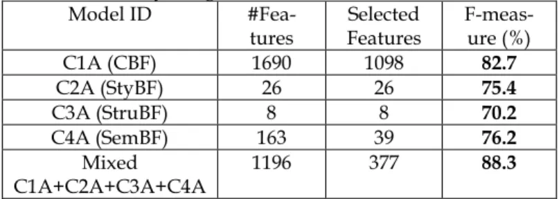
Table 6. Classification by Arousal Hemispheres: Combination of the best models by categories.

Model ID

#Fea-tures

Selected Features

F-meas-ure (%)

C1A (CBF) 1690 1098 82.7

C2A (StyBF) 26 26 75.4

C3A (StruBF) 8 8 70.2

C4A (SemBF) 163 39 76.2

Mixed C1A+C2A+C3A+C4A

1196 377 88.3

4.2.3 Classification by Valence Meridians

We perform the same study for the classification by valence me-ridian. The following table (Table 7) shows the results of the best models by type of features.

Table 7. Classification by Valence Meridians: Best F-measure re-sults for model.

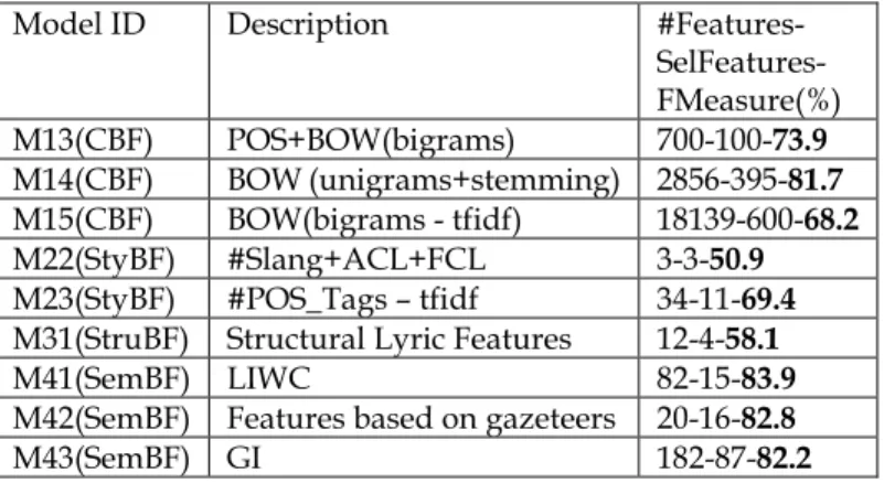
Model ID Description

#Features- SelFeatures-FMeasure(%)

M13(CBF) POS+BOW(bigrams) 700-100-73.9

M14(CBF) BOW (unigrams+stemming) 2856-395-81.7

M15(CBF) BOW(bigrams - tfidf) 18139-600-68.2

M22(StyBF) #Slang+ACL+FCL 3-3-50.9

M23(StyBF) #POS_Tags – tfidf 34-11-69.4

M31(StruBF) Structural Lyric Features 12-4-58.1

M41(SemBF) LIWC 82-15-83.9

M42(SemBF) Features based on gazeteers 20-16-82.8

M43(SemBF) GI 182-87-82.2

These results show the importance of the semantic features in general, since the semantic models (M41, M42, M43) are signifi-cantly better than the classifiers of the other types of features (at p < 0.05). Features related with the positivity or negativity of the words such as VinDAL or posemo (positive words) have an im-portant role to these results.

Table 8 shows the combinations by feature sets and the com-bination of the comcom-binations respectively.

Table 8. Classification by Valence Meridians: Combination of the best models by category.

Model ID #Features Selected

Features

F-measure (%)

C1V (CBF) 1095 750 85.6

C2V (StyBF) 14 11 71

C3V (StruBF) 4 4 58.1

C4V (SemBF) 39 6 86.7

Mixed C1V+C2V+C3V+C4V

771 594 90

In comparison to the previous studies (quadrants and arousal), these results are better in general. We can see this in the BOW experiments (baseline-85.60%) where we achieved a performance close to the best combination (C4V). The best re-sults are also in general achieved with less features as we can see in C3V and C4V.

The mixed classifier (90%) is significantly better than the best classifiers by type of feature: C1V, C2V, C3V and C4V (at p < 0.05).

4.2.4 Binary Classification

As a complement to the multiclass problem seen previously, we also evaluated a binary classification (BC) approach for each emotion category (e.g., quadrant 1). Negative examples of a cat-egory are lyrics that were not tagged with that catcat-egory but were tagged with the other categories. For example (see Table 9) the BC in the quadrant 1 uses 88 examples, 44 positive examples and 44 negative examples. The latter 44 examples are equally distrib-uted by the other quadrants.

The results in Table 9 were reached using 396, 442, 290 and 696 features, respectively for the four sets of emotions (quad-rants).

Table 9 - F-measure values for BC.

Sets of Emotions #lyrics F-measure (%)

Quadrant 1 88 88.6

Quadrant 2 82 91.5

Quadrant 3 102 90.2

Quadrant 4 88 88.6

The good performance of these classifiers, namely for quad-rant 2, indict that the prediction models can capture the most important features of these quadrants.

The analysis of the most important features by quadrant will be the starting point for the identification of the best features by sets of emotions or quadrants, as detailed in section 4.4.

4.3 New Features: Comparison to Baseline

Considering CBF as the baseline in this area, we though it would be important to assess the performance of the models created when we add to the baseline the new proposed features. The new proposed features are contained in three categories: StyBF (feature set M22), StruBF (feature set M31) e SemBF (feature set M42). Next, we created new models adding to C1* each one of the previous feature sets in the following way: C1*+M22; C1*+M31; C1*+M42; C1*+M22+M31+M42. In C1*, ‘C1’ denotes a feature set that contains the combination of the best Content-Based Features – baseline and ‘1’ denotes CBF, as mentioned above; “*” denotes expansion notation, indicating the different experiments conducted: Q denotes classification by quadrants, A by arousal hemispheres and V by valence meridians. These models were created for each of the 3 classification problems seen in the previous section: Classification by quadrants (see Ta-ble 10); classification by arousal (see TaTa-ble 11); classification by valence (see Table 12).

Table 10. Classification by quadrants (baseline + new features).

Model ID Selected

Features

F-measure (%)

C1Q+M22 384 72.1

C1Q+M31 466 70.4

C1Q+M42 576 78.4

C1Q+M22+M31+M42 388 82.7

The baseline model (C1Q) alone reached 69.9% with 812 fea-tures selected (Table 4). We improve the results with all the

com-binations but only the models C1Q+M42 and

C1Q+M22+M31+M42 are significantly better than the baseline model (at p < 0.05). However the model C1Q+M22+M31+M42 is significantly better (at p < 0.05) than the model C1Q+M42. This shows that the inclusion of StruBF and StyBF have im-proved overall results.

Table 11. Classification by arousal (baseline + new features).

Model ID Selected

Features

F-measure (%)

C1A+M22 652 83.3

C1A+M31 373 83.3

C1A+M42 690 84.4

The baseline model (C1A) alone reached an F-measure of 82.7% with 1098 features selected (Table 6). We improve the re-sults with all the combinations but only the models C1A+M42 and C1A+M22+M31+M42 are significantly better than the base-line model (at p < 0.05). The inclusion of the features from M22 and M31 in C1A+M22+M31+M42 improved the performance in comparison to the model C1A+M42, since C1A+M22+M31+ M42 is significantly better than the model C1A+M42 (at p < 0.05).

Table 12. Classification by valence (baseline + new features).

Model ID Selected

Features

F-measure (%)

C1V+M22 679 85

C1V+M31 659 83.9

C1V+M42 493 87.8

C1V+M22+M31+M42 88 88.3

The baseline model (C1V) alone reached an F-measure of 85.6% with 750 features selected (Table 8). We improve the re-sults with all the combinations but only the models C1V+M42 and C1V+M22+M31+M42 are significantly better than the base-line model (at p < 0.05), however C1V+M22+M31+M42 is not significantly better than C1V+M42. This suggests the im-portance of the SemBF for this task in comparison to the other new features.

In general, the new StyBF and StruBF are not good enough to improve significantly the baseline score, however we got the same results with much less features: for classification by quad-rants we decrease the number of features of the model from 812 (baseline) to 384 (StyBF) and 466 (StruBF). The same happens for arousal classification (1098 features - baseline to 652 - StyBF and 373 – StruBF) and for valence classification (750 features – base-line to 679 – StyBF and 659 – StruBF).

However, the model with all the features is always better (ex-cept for valence classification) than the model with only baseline and SemBF. This shows a relative importance of the novel StyBF and StruBF. It is important to highlight that M22 has only 3 fea-tures and M31 has 12 feafea-tures.

The new SemBF (model M42) seems important because it can improve clearly the score of the baseline. Particularly in the last problem (classification by valence) it requires a much less num-ber of features (750 down to 88).

4.4 Best Features by Classification Problem

We determined in the previous section the classification models with best performance for the several classification problems. These models were built through the interaction of a set of fea-tures (from the total of feafea-tures after feature selection). Some of these features are possibly strong to predict a class when they are alone but others are strong only when combined with other features.

Our purpose in this section is to identify the most important features, when they act alone, for the description and discrimi-nation of the problem’s classes.

We will determine the best features for:

 Arousal (Hemispheres) description – the classes used are negative arousal (AN) and positive arousal (AP)  Valence (Meridians) description - negative valence

(VN) and positive valence (VP)

 Arousal when valence is positive – negative arousal

(AN) and positive arousal (AP), which means quad-rant 1 vs quadquad-rant 4

 Arousal when valence is negative – negative arousal (AN) and positive arousal (AP), which means quad-rant 2 vs quadquad-rant 3

 Valence when arousal is positive – negative valence (VN) and positive valence (VP), which means quad-rant 1 vs quadquad-rant 2

 Valence when arousal is negative – negative valence (VN) and positive valence (VP), which means quad-rant 3 vs quadquad-rant 4

In all the situations we identify the 5 features that, after anal-ysis, seem the best features. This analysis starts from the rank-ings (top 20) of the best features extracted from the models of the section 4.2, with ReliefF. Next, to validate ReliefF’s ranking, we compute the probability density functions (pdf) [31] for each of the classes of the previous problems. Through the analysis of these pdfs we take some conclusions about the description of the classes and identify some of their main characteristics.

The images below show the pdfs of 2 of the 5 best features for the problem of valence description when the arousal is positive (distinguish between 1st _{quadrant and 2}nd _{quadrant) (Figure 4).}

The features are M44-Anger_Weight_Synesketch (a) and M42-Di-nANEW (b).

(a)

(b)

Figure 4. pdf of the features a) Anger_Weight_Synesketch and b) DinANEW for the problem of valence description when arousal is positive.

As we can see, the feature in the top image is more important for discriminating between the 1st _{and 2}nd _{quadrants than the}









B A

B A

f f

f f on_Area Intersecti

 

(2)

In (2), A and B are the compared classes (VN and VP in the example of the Figure 4) and fAand fBare respectively the pdfs for A and B.

For this measure, lower values indicate more separation be-tween the curves.

Both features are important to describe the quadrants. The first, taken from the Synesketch framework measures the weight of anger in the lyrics and, as we can see, it has higher values for the 2nd _{quadrant as expected, since anger is a typical emotion}

from the 2nd _{quadrant. The 2}nd _{feature represents the average}

dominance of the ANEW’s words in the lyrics and, although some overlap, it shows that predominantly higher values indi-cate the 1st _{quadrant and lower values indicate the 2}nd _quadrant.

Based on above metric, the top-5 best features were identified for each problem, i.e., the features that separate better the differ-ent problems.

4.4.1 Best Features for Arousal Description

As we can see (Table 13), the two best features to discriminate between arousal hemispheres are new features proposed by us. FCL represents the number of words started by a capital letter and it describes better the class AP than the class AN, i.e., lyrics with FCL greater than a specific value correspond normally to lyrics from the class AP. For low values there is a mix between the 2 classes. The same happens to #Slang, #Title, WC (word count - LIWC), active (words with active orientation – GI) and vb (number of verbs in the base form). The feature negate (number of negations – LIWC) has an opposite behavior, i.e., mix between classes for lower values and the class AN from a specific point. The features not listed above, sad (words of the negative emotion sadness – LIWC), angry (angry weight in ConcepNet) and numb (words indicating the assessment of quantity, including the use of numbers – GI) have a similar pattern of behavior as the fea-ture negate, while the novel features CH (number of repetitions of the chorus) and TotalVorCH (number of repetitions of verses or chorus) have similar pattern of behavior as the feature FCL.

Table 13. Best features for arousal description (classes AN, AP).

Feature Intersection Area

M22-FCL 24.6%

M22-#Slang 29%

M43- active 33.1%

M21- vb 34.2%

M31-#Title 37.4%

4.4.2. Best Features for Valence Description

The best features and not only the 5 on Table 14, are essentially semantic features. The feature VinDAL can describe both classes: lower values are more associated to the class VN and higher val-ues to the class VP. The feature DinANEW has a similar pattern but not so good. The features VinGAZQ1Q2Q3Q4, negemo (words associated with negative emotions - LIWC), negativ (words of negative outlook – GI) and VinANEW are better for discrimination of the VN class. For the VP class they are not so good. The feature posemo (number of positive words – LIWC) for example describes better the VP class.

Table 14. Best features for valence description (classes VN, VP).

Feature Intersection Area

M41- posemo 18.5%

M43- negativ 24.8%

M42-VinDAL 25.6%

M42-VinGAZQ1Q2Q3Q4 25.8%

M42- VinANEW 26.1%

4.4.3. Best Features For Arousal when Valence is Positive. As can be seen in Table 15, the features #GAZQ1, FCL, iav (verbs giving an interpretative explanation of an action – GI), motion (measures dimension motion – LIWC), vb (verbs in base form, vbn (verbs in past participle), active, you (pronouns indicating another person is being addressed directly – GI) and #Slang are good for discrimination of the 1st _{quadrant (higher values}

asso-ciated to the class AP).

The features angry_CN, numb and article (number of articles – LIWC) are good for discrimination of the 4th _{quadrant. The}

fea-ture AinGAZQ1Q2Q3Q4 is good for both quadrants.

Table 15. Best features for arousal (V+) (classes AN, AP).

Feature Intersection Area

M42-#GAZQ1 4.6%

M43- active 12.5%

M21- vbn 17.6%

M43- you 17.8%

M21- vb 18.7%

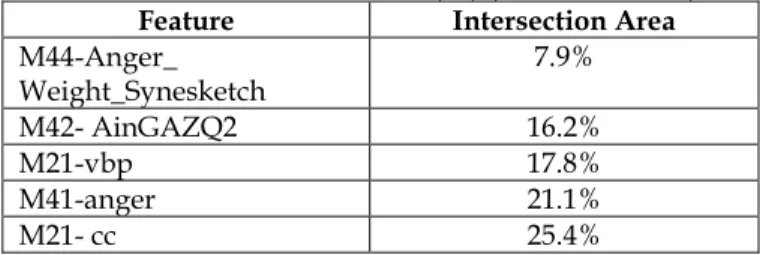
4.4.4 Best Features for Arousal when Valence is Negative These features are summarized in Table 16. The features An-ger_Weight_Synesketch and Disgust_Weight_Synesketch (weight of the emotion disgust) are good to discriminate between the quad-rants 2 and 3 (higher values are associated as it was predictable to instances from the quadrant 2), although in the latter we have more overlap between the classes than in the prior. The features vbp (verb, non-3rd person singular present) and anger can dis-criminate the class AP (higher values) but for lower values we have a mix between the classes. Other features with similar be-havior are FCL, #Slang, negativ (negative words - GI), cc (number of coordinating conjunctions) and #Title. AinGAZQ2 and past can discriminate the 3rd _{quadrant, i.e., the class AN. Finally the}

feature article (the number of definite, e.g., the, and indefinite, e.g., a, an, articles in the text) can discriminate both quadrants (tendency for 3rd _{quadrant with lower values and 2}nd _quadrant

with higher values).

Table 16. Best features for arousal (V-) (classes AN, AP).

Feature Intersection Area

M44-Anger_ Weight_Synesketch

7.9%

M42- AinGAZQ2 16.2%

M21-vbp 17.8%

M41-anger 21.1%

4.4.5 Best Features for Valence when Arousal is Positive. The feature Anger_Weight_Synesketch is clearly discriminative to separate the quadrants 2 and 3 (see Table 17 and Figure 4). The novel semantic features VinANEW, VinGAZQ1Q2Q3Q4, VinDAL and DinANEW have a similar pattern behavior to the first feature but with a little overlap between the functions. The features negemo (negative emotion words – LIWC), swear (swear words – LIWC), negative (words of negative outlook – GI) and hostile (words indicating an attitude or concern with hostility or aggressiveness – GI) are good for the discrimination of the 2nd

quadrant (higher values).

Table 17. Best features for valence (A+) (classes VN, VP).

Feature Intersection Area

M44-Anger_ Weight_Synesketch

0.1%

M42- VinANEW 4.4%

M42- VinGAZQ1Q2Q3Q4 7.2%

M42- VinDAL 7.7%

M42- DinANEW 10.7%

4.4.6. Best Features for Valence when Arousal is Negative. The best features for valence discrimination when arousal is negative are presented in Table 18.

Between the quadrants 3 and 4, the features vbd, I, self and motion are better for the 3rd _{quadrant discrimination, while the}

features #GAZQ4, article, cc and posemo are better for 4th

quad-rant discrimination.

Table 18. Best features for valence (A-) (classes VN, VP).

Feature Intersection Area

M41- posemo 15.6%

M43- self 24.9%

M21-vbd 27%

M42-#GAZQ4 28.4%

M41- motion 29.2%

4.4.7. Best Features by Quadrant

Until now we have identified features important to discrimi-nate, for example, between two quadrants. Next, we will evalu-ate if these features can discriminevalu-ate completely the four quad-rants, i.e., one quadrant against the other three.

To evaluate the quality of the discrimination of a specific fea-ture concerning a quadrant Qz, we have established a metric based on two measures:

 Discrimination support (support of a function is the set of points where the function is not zero-valued [33]), which corresponds to the difference between the total support of the two pdf (Qz and Qothers) and the support of the Qothers pdf, as defined in (3). The re-sult is the support of the Qz pdf except the support of the intersection area and is in percentage of the total support. The higher this metric the better;

























others others

Z

Q Q

Q Q

Q

f f len

f len f

f len Disc

 

sup

sup sup

sup

_   (3) In (3), len(sup(f)) stands for the length of the support of func-tion f and fQ_Zand fQ_others are respectively the pdfs for Qz and

Qothers.

 Discrimination area, which corresponds to the differ-ence between the area of the Qz’s pdf and the intersec-tion area between the two pdf, as in (4). The result is in percentage of the Qz’s pdf total area. The higher this metric the better (Equation 4).









Z

others Z

Z

Q Q Q Q

f f f f

area Disc



_ (4)

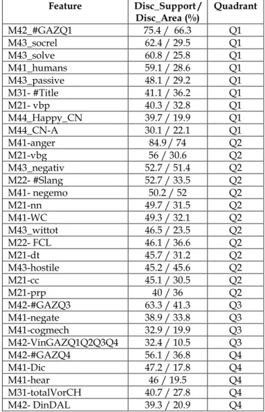
In this analysis (Table 19), we have experimentally de-fined a minimum threshold of 30% for the Discrimination_Sup-port. To do the ranking of the best features, we use the metric Discrimination_support and in case of a draw, we use the met-ric Discrimination_Area.

Table 19. Type of discrimination of the features by quadrant.

Feature Disc_Support /

Disc_Area (%)

Quadrant

M42_#GAZQ1 75.4 / 66.3 Q1

M43_socrel 62.4 / 29.5 Q1

M43_solve 60.8 / 25.8 Q1

M41_humans 59.1 / 28.6 Q1

M43_passive 48.1 / 29.2 Q1

M31- #Title 41.1 / 36.2 Q1

M21- vbp 40.3 / 32.8 Q1

M44_Happy_CN 39.7 / 19.9 Q1

M44_CN-A 30.1 / 22.1 Q1

M41-anger 84.9 / 74 Q2

M21-vbg 56 / 30.6 Q2

M43_negativ 52.7 / 51.4 Q2

M22- #Slang 52.7 / 33.5 Q2

M41- negemo 50.2 / 52 Q2

M21-nn 49.7 / 31.5 Q2

M41-WC 49.3 / 32.1 Q2

M43_wittot 46.5 / 23.5 Q2

M22- FCL 46.1 / 36.6 Q2

M21-dt 45.7 / 31.2 Q2

M43-hostile 45.2 / 45.6 Q2

M21-cc 45.1 / 30.5 Q2

M21-prp 40 / 36 Q2

M42-#GAZQ3 63.3 / 41.3 Q3

M41-negate 38.9 / 33.8 Q3

M41-cogmech 32.9 / 19.9 Q3

M42-VinGAZQ1Q2Q3Q4 32.4 / 10.5 Q3

M42-#GAZQ4 56.1 / 36.8 Q4

M41-Dic 47.2 / 17.8 Q4

M41-hear 46 / 19.5 Q4

M31-totalVorCH 40.7 / 27.8 Q4

M42- DinDAL 39.3 / 20.9 Q4

socrel (words for socially-defined interpersonal processes), solve (words referring to the mental processes associated with prob-lem solving), passive (words indicating a passive orientation), negativ (negative words) and hostile (words indicating an atti-tude or concern with hostility or aggressiveness); from Concep-Net (M44) - happy_CN (happy weight), CN_A (arousal weight); from POS Tags (M21) –vbp (verb, non-3rd person singular pre-sent), vbg (verb, gerund or present participle), nn (noun, singular or mass), dt (determiner), cc (coordinating conjunction) and prp (personal pronoun). We have also novel features, such as, StyBF (M22) –#Slang and FCL; StruBF (M31) - #Title and TotalVorCH; SemBF (M42) - #GAZQ1, #GAZQ3, VinGAZQ1Q2Q3Q4, #GAZQ4 and DinDAL.

Some of the more salient characteristics of each of the quad-rants:

 Q1: typically lyrics associated to songs with positive emotions and high activation. Songs from this quadrant are often associated to specific musical genres, such as, dance, pop and by the importance of the features we point out the features related with repetitions of the chorus and title in the lyric.

 Q2: we point out stylistic features such as #Slang and FCL that indict high activation with predominance of negative emotions or features that are related with neg-ative valence such as negativ (negative words), hostile (hostile words) and swear (swear words). This kind of features influence more Q2 than Q3 (although Q3 have also negative valence) because Q2 is more influenced by specific vocabulary such as the vocabulary in that features, while Q3 is more influenced by negative ideas, so we think that it is more difficult the perception of emotions in the 3rd _quadrant.

 Q3: we point out the importance of the verbal tense (past) in comparison with the other quadrants which have the predominance of the present tense. On the contrary, Q2 have also some tendency to the gerund tense and the Q1 to the present simple. We highlight also in comparison with the other quadrants more use of the 1st _{singulier person (I).}

 Q4: Features related with activation, as we have seen for the quadrants 1 and 2, have low weight for this quadrant. We point out the importance of a specific vo-cabulary as we have in #GAZQ4.

Generally, semantic features are more important to discrimi-nate the valence (e.g. VinDAL, VinANEW). Features important for sentiment analysis such as posemo (positive words) or ngtv (negative words) are also important for valence discrimination. On the other hand, stylistic features related with the activa-tion of the written text such as #Slang or FCL are important for arousal discrimination. Features related with the weight of emo-tions in the written text are also important (e.g. An-ger_Weight_Synesketch, Disgust_Weight_Synesketch).

4.5 Interpretability

After we have made a study to understand the best features to describe and discriminate each set of emotions, we are going to extract some rules/knowledge that allow to understand how these features and emotions are related. With this study we in-tend to attain two possible goals: i) find out relations between features and emotions (e.g., if feature A is low and feature B is

high then the song lyrics belong to quadrant 2); ii) find out rela-tions among features (e.g., song lyrics with feature A high also have feature B low).

4.5.1 Relations between features and quadrants In this analysis we use the Apriori algorithm [34].

First, we pre-processed the employed features through the detection of features with a nearly uniform distribution, i.e., the feature values depart at most 10% from the feature mean value. We did not consider these kind of features. Here, we employed all the features selected in Mixed C1Q + C2Q + C3Q + C4Q model (see Table 4), except for the ones excluded as described. In total, we employed 144 features.

Then we defined the following premises.

 Consideration of only rules up to 2 antecedents. It was applied an algorithm to eliminate redundance, consid-ering the more generic rules to avoid complex rules;  Due to the fact that n-grams features are sparse, we

did not consider rules with part of the antecedent of type n-gram = Very Low. It means probably that the feature does not exist;

 Features were discretized in 5 classes using equal-fre-quency discretization: very low (VL), low (L), medium (M), high (H), very high (VH). Rules containing non-uniform distributed features were ignored.

We considered two measures to assess the quality of the rules: confidence and support. The ideal rule has simultane-ously high representativity (support) and high confidence de-gree.

Table 20 shows up the best rules for quadrants. We defined a threshold of support = 8.3% (15 lyrics) and confidence = 60%.

We think this rules are in general self-explanatory and under-standable, however we will explain some of them not so explicit.

We can see for Q1 the importance of the feature #GAZQ1 to-gether with the feature from GI, afftot (words in the affect do-main), both with VH values. We can also highlight for this quad-rant the relation between a VL weight for sadness and a VH value for the feature positiv (words of positive outlook) and the rela-tion between a VH number of title’s repetitions in the lyric and a VL weight for the emotion angry.

We can point out for quadrant 2 the importance of the fea-tures anger from LIWC and Synesketch, negemo_GI (negative emotion), #GAZQ2, VinANEW, hostile (words indicating an atti-tude or concern with hostility or aggressiveness), powcon (words for ways of conflicting) and some combinations among them.

For quadrant 3, we can point out the relation between a VH value for the emotion sadness and a VL value for the number of swear words in the lyrics.

For quadrant 4 we can point out the relation between the fea-tures anger and weak (words implying weakness) both with VL values.

These results confirm the results reached in the previous sec-tion, where we identified the most important features for each quadrant.

Table 20. Rules from classification association mining.

# Rule Support/

confidence (%)

1 #GAZQ1=VH ==> Q=Q1 13.8 / 80

2 #GAZQ1=VH and afftot_GI=VH => Q1

3 sad_LIWC=VL and positiv_GI=VH => Q1

7.7 / 82

4 #Title=VH and angry_CN=VL => Q1 7.2 / 72

5 VinANEW=VL => Q2 20 / 61

6 hostile_GI=VH and

Sad-ness_Weight_Synesketch=VH => Q2

14.4 / 69

7 Anger_Weight_Synesketch=VH and Valence_Synesketch=VL => Q2

12.7 / 76

8 anger_LIWC=H => Q2 11.1 / 85

9 negemo_GI=VH => Q2 11.1 / 67

10 #GAZQ2=VH => Q2 10.5 / 100

11 Anger_Weight_Synesketch=VH and negemo_LIWC=VH => Q2

8.8 / 94

12 anger_LIWC=VH => Q2 8.8 / 100

13 VinGAZQ2=VH => Q2 8.3 / 83

14 hostile_GI=VH and powcon_GI=VH => Q2

8.3 / 78

15 sad_LIWC=VH and swear_LIWC=VL => Q3

8.8 / 72

16 dt=VL and article_LIWC=VL => Q3 8.3 / 71 17 dt=VL and Valence_Synesketch=VL

=> Q3

8.3 / 71

18 anger_LIWC=VL and weak_GI=VL => Q4

10 / 72

19 swear_LIWC=VL and #GAZQ4=VH

=> Q4

9.4 / 73

20 #Slang=VL and #GAZQ2=VL => Q4 8.8 / 76 21 prp=VL and #GAZQ2=VL => Q4 8.8 / 72

4.5.2 Relations among features

The same premises concerning outliers, false predictors and dis-cretization were applied as in the prior section.

We have considered rules with a minimum representativity (support) of 10% and a minimum confidence measure of 95%. After that all the rules were analyzed and redundant rules were removed.

The results (Table 21) show only the more representative rules and are in consonance with what we suspected after the analysis made in the last sections.

We briefly analyze the scope of the rules listed in Table 21. (Rule 1) The feature GI_passive (words indicating a passive orientation) has, for the class VH, almost all the songs in the quadrants 1 and 2. The same happens for the features vb (verb in base form) and prp (personal pronouns). We would say that this rule reveals an association among the features namely for positive activation.

(Rule 2) GI_intrj (includes exclamations as well as casual and slang references, words categorized "yes" and "no" such as "amen" or "nope", as well as other words like "damn" and "fare-well") and GI_active (words implying an active orientation) both with values very high imply a VH value for the feature GI_iav (verbs giving an interpretative explanation of an action, such as "encourage, mislead, flatter"). This rule is predominantly true for the quadrant 2.

Table 21. Rules from association mining.

# Association rules Support/

Confidence (%) 1 GI_passive=VH and vb=VH => prp=VH 20 / 100

2 GI_intrj=VH and GI_active=VH => GI_iav=VH

19 / 100

3 #Slang=VH and GI_you=VH => prp=VH 18 / 100 4 VinANEW=VL and Fear_W_Syn=VH =>

Sadness_W_Syn=VH

18 / 100

5 #Slang=VH and FCL=VH and dav=VH => WC=VH

18 / 100

6 strong=VH and GI_active=VH => iav=VH

22 / 95

7 #Slang=VL and prp=VL => WC=VL 21 / 95

8 #Slang=VL and FCL=VL => WC=VL 21 / 95

9 vb=VH and GI_you=VH => prp=VH 21 / 95

10 #Slang=VH and jj=VH => WC=VH 19 /95

11 VinGAZQ1Q2Q3Q4=VL and Fear_W_Syn=VH => Sad-ness_W_Syn=VH

19 / 95

12 #Slang=VL and active=VL => strong=VL 19 / 95 13 FCL=VH and active=VH => iav=VH 19 / 95

(Rule 3) the features #Slang and you (pronouns indicating an-other person is being addressed directly) have higher values for quadrant 2 and this implicate and higher number of prp in the written style. This is typical from genres like hip-hop.

(Rule 4) Almost all the samples with a value VL for the fea-ture VinANEW are in the quadrants 2 (more) and 3 (less). Fear_Weight_Synesketch has a VH value essentially in the quad-rant 2. Sadness_Weight_Synesketch has higher values for quad-rants 3 and 2, so probably this rule is applied more on songs of quadrant 2.

(Rule 5) We can see the association among the features #Slang, FCL, dav (verbs of an action or feature of an action, such as run, walk, write, read) and WC (word count), all of them with high values and we know that this rule is more associated with the 2nd _quadrant.

(Rule 6) This rule is more associated to the quadrants 1 and 2. High values for the features strong (words implying strength), active and iav

(Rules 7 and 8) Almost all the songs with #Slang, prp, FCL and WC equal to VL, belong to the quadrants 3 and 4.

(Rule 9) The feature vb has higher values for quadrant Q2 fol-lowed by quadrant Q1 while feature you has higher values for quadrant Q2 followed by the quadrant 3. Prp with VH values is predominantly in the quadrant 2, so this rule is probably more associated to the quadrant 2.

(Rule 10) These features, #Slang, jj (number of adjectives) and WC have VH values essentially for the quadrants 1 and 2.

(Rule 11) This rule is probably more applied in the quadrants 2 or 3, since the feature VinGAZQ1Q2Q3Q4 has predominantly lower values for quadrants 2 and 3, while Fear_Weight_ Synesketch has higher values in the same quadrants.

(Rule 12) The three features have VL values essentially for the quadrants 3 and 4.

(Rule 13) The three features have VH values essentially for the quadrants 1 and 2.

5

C

F

W