Orientador: José Manuel Fonseca, Professor Auxiliar, FCT-UNL Co-orientador: André Sanches Ribeiro, Professor Assistente, TUT, Finlândia

(1)

Leonardo Pedro Donas

-

Boto de Vilhena Martins

Licenciatura em Ciências de Engenharia Biomédica

STOCHASTIC MODEL OF

TRANSCRIPTION INITIATION OF

CLOSELY SPACED PROMOTERS IN

ESCHERICHIA COLI

Dissertação para obtenção do Grau de Mestre em Engenharia Biomédica

Orientador: José Manuel Fonseca, Professor Auxiliar, FCT-UNL

Co-orientador: André Sanches Ribeiro, Professor Assistente, TUT, Finlândia

Júri:

Prof. Doutor Mário António Basto Forjaz Secca Prof. Doutora Ilda Santos Sanches

Prof. Doutor José Manuel Fonseca Prof. Doutor André Sanches Ribeiro

Dezembro 2011

(2)

(3)

Martins. Faculdade de Ciências e Tecnologia. Universidade Nova de Lisboa.

A Faculdade de Ciências e Tecnologia e a Universidade Nova de Lisboa têm o direito,

perpétuo e sem limites geográficos, de arquivar e publicar esta dissertação através de exemplares

impressos reproduzidos em papel ou de forma digital, ou por qualquer outro meio conhecido ou

que venha a ser inventado, e de a divulgar através de repositórios científicos e de admitir a sua

cópia e distribuição com objectivos educacionais ou de investigação, não comerciais, desde que

(4)

(5)

“Aut inveniam viam aut faciam”

(6)

(7)

Resumo

Os mecanismos reguladores da transcrição permitem aos organismos uma rápida adaptação a mudanças no meio ambiente e actuam frequentemente na iniciação da transcrição. Nesta Tese é proposto um modelo estocástico da iniciação da transcrição ao nível dos nucleotídos para estudar a dinâmica da produção de ácidos ribonucleicos (RNAs) em promotores com um curto espaçamento e os seus mecanismos de regulação.

Neste estudo analisa-se como diferentes disposições (convergente e divergente), distância entre os locais de iniciação da transcrição (TSS) e diferentes parâmetros cinéticos afectam a dinâmica da produção de RNAs e como diferentes passos na iniciação da transcrição podem ser regulados variando os locais de ligação do repressor.

Através dos resultados, observa-se que os passos que limitam a produção podem ter uma grande influência na cinética da produção de RNAs nas duas disposições. Descobre-se que uma maior interferência entre as RNA polimerases nos promotores divergentes com sobreposição e nos convergentes, aumentam a média e desvio padrão da distribuição dos intervalos de tempo entre produção de RNAs, provocando uma maior oscilação nos níveis de RNA.

Observa-se também que pequenas mudanças na distância entre os TSS podem provocar transições abruptas na dinâmica da produção de RNAs, principalmente na transição entre promotores com e sem sobreposição.

Dos estudos da correlação mostra-se que através da afinação das distâncias entre os TSS nas diversas disposições se pode obter tanto uma correlação negativa como positiva, quer na direccionalidade de RNAs consecutivos como nas séries temporais. Também se mostra que mecanismos de repressão distintos do início da transcrição, em tais passos como a formação dos complexos fechados e abertos e a libertação do promotor, têm diferentes efeitos na dinâmica da produção de RNAs.

Este tipo de modelos podem ajudar a explicar como os circuitos genéticos evoluíram, podendo ainda ajudar a produzir circuitos genéticos com propriedades específicas.

(8)

(9)

Abstract

The regulatory mechanisms of transcription allow organisms to quickly adapt to changes in their environment and often act during transcription initiation. Here, a stochastic model of transcription initiation at the nucleotide level is proposed to study the dynamics of RNA production in closely spaced promoters and their regulatory mechanisms.

We study how different arrangements (convergent e divergent), distance between transcription start sites (TSS), and various kinetic parameters affect the dynamics of RNA production. Further, we analyze how the kinetics of various steps in transcription initiation can be regulated by varying locations of repressor binding sites.

From the results, we observe that the rate limiting steps have strong influence in the kinetics of RNA production. We find that interferences between RNA polymerases in divergent overlapped and convergent geometries causes the distribution of time intervals between the production of consecutive RNA molecules from each TSS to increase in mean and standard deviation, which leads to stronger fluctuations in the temporal levels of RNA molecules.

We observe that small changes in the distance between TSSs can lead to abrupt transitions in the dynamics of RNA production, particularly when this change changes the geometry from overlapped to non-overlapped promoters.

From the study of the correlation in the choices of directionality and on the time series of RNA productions we show that by tuning the distances and directions of the two TSS one can obtain both negative and positive correlations. We further show that distinct repression mechanisms of transcription initiation in steps such as the open and closed complex formation and promoter escape have different effects on the dynamics of RNA production.

The study of these models will help the study of how genetic circuits have evolved and assist in designing artificial genetic circuits with desired dynamics.

(10)

(11)

Acknowledgements

First, I would like to thank my supervisor Prof. Dr. José Manuel Fonseca, who offered me this great opportunity of doing my Master Thesis project and gave me a great support.

To Prof. Dr. André Sanches Ribeiro, who welcomed me in his group and provided a great assistance during my stay, both at supporting and providing me with all the tools necessary for this work.

To Jarno Mäkelä, who helped me a lot during this Thesis, especially in the section of the results, where we discussed what type of results we needed for this work.

To Jason Lloyd-Price and Antti Häkkinen who provided me with the tools necessary for this work. Jason gave me the SGNS simulator, where we made all ours simulations and gave me some important insights in stochastic simulations which I used in the Chapter 2.1. Antti gave me a template of a model in which I created this model for transcription initiation.

To Abhishekh Gupta, who were always present and occupying the “Grid”, but also helped

me find a home in Finland and invited me to so many sport games with his friends.

To everyone in the LBD group, who were always there to help me but also provided for times of fun and relaxation, especially during Bomberman.

To all my friends and especially the ones I met 5 years ago, when we all started our studies in Biomedical Engineering, because they made this 5 year journey so much more fun and pleasant. Joaquim Horta, Hugo Pereira, Sérgio Mendes, Pedro Martins, Luís Mendes, Fernando Mota, Bernardo Azevedo, Nuno Fernandes, Filipe Oliveira, João Martins, Pedro Cascalho, João Santinha, Mafalda Fernanda, Ana Frazão, Sara Gil, Rita Rosa, Ana Marques, Ana Margarida, Susana Gaspar, Susana Martinho, Cátia Rocha, Milene Bação, and to everyone else I want to show my greatest gratitude for all the good times spent with you guys and hopefully we shall continue this great friendship after completing this journey together. A picture is worth a thousand words, but sometimes we just need 4 to express our feelings: I love you guys!!!

A special thanks to Joaquim and João Santinha for sharing their house with all their friends in the all night studies or just when we needed a warm couch.

(12)

(13)

Abbreviations and Symbols

λ phage Lambda bacteriophage

( ) Propensity function

APR Abortive to productive ratio

bp Base pairs

CME Chemical master equation

CV Coefficient of variation

DNA Deoxyribonucleic acid

EC Elongation complex

E. coli Escherichia coli

FF Fano Factor

FRET Förster resonance energy transfer

In vivo Latin for “within the living”

In vitro Latin for “within glass”

ITC Initial transcribing complex

( ) Possible reactant combinations in the reaction volume

ODE Ordinary Differential Equation

RNA Ribonucleic acid

RNAp Ribonucleic acid polymerase

RPc Closed complex of RNA polymerase and the DNA

RPi Isomerized complex of RNA polymerase and the DNA

RPo Open complex of RNA polymerase and the DNA

RRE Reaction Rate Equation

SSA Stochastic simulation algorithm

TFBS Transcription factor binding site

TSS Transcriptional start site

UV Ultraviolet

(14)

(15)

Figure contents

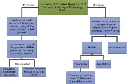
Figure 1.1 – Scheme with the objectives of this work (left side), the motivation behind this

work (right side) and the location where this work was done (green box). ... 3

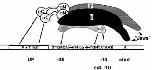
Figure 2.1 – The interaction between the subunits of RNAp and the core promoter. The

consensus sequences for the -10 and -35 promoter motifs and the “UP element” are also shown.

The contacts between RNAp and the promoter are shown in solid lines. Figure taken from [54]. ... 9

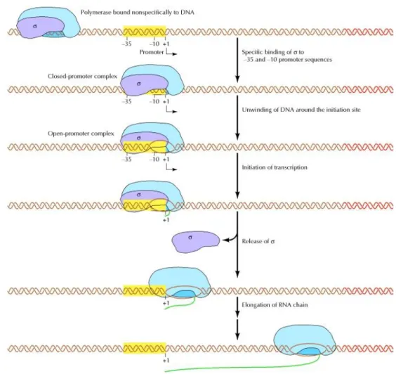
Figure 2.2 – The RNAp can bind nonspecifically to DNA and searches for the promoter.

The σ70_{subunit recognizes to the -35 and -10 promoter motifs and forms a closed-promoter}

complex. The RNAp then unwinds DNA around the initiation site forming an open complex. Then

transcription is initiated followed by the release of sigma and the elongation of the RNA chain.

Figure taken from [70]. ... 11

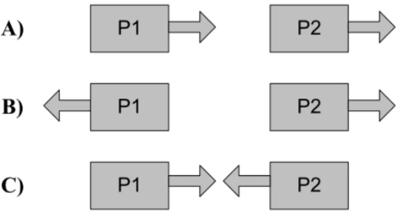
Figure 2.3 – Possible types of closely spaced promoter arrangements. There are three types

of arrangements: tandem (A), divergent (B), convergent (C) promoters. ... 12

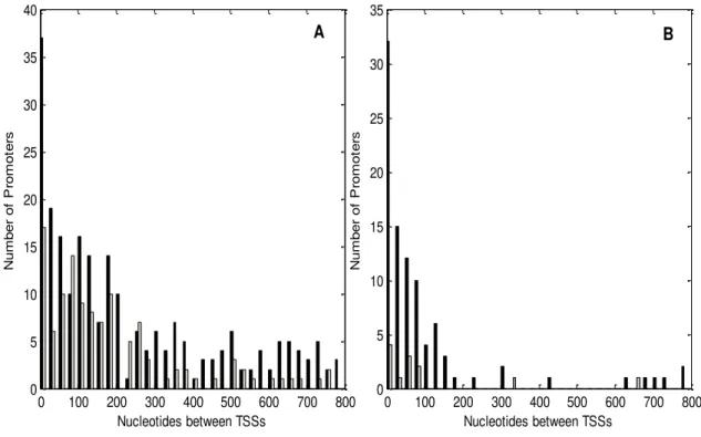
Figure 2.4 – Numbers of promoters pairs with a given number of nucleotides between the

TSSs for (A) divergent promoters, and (B) convergent promoters. Gray bars are used for the known

promoters and black bars are used for the predicted promoters. ... 14

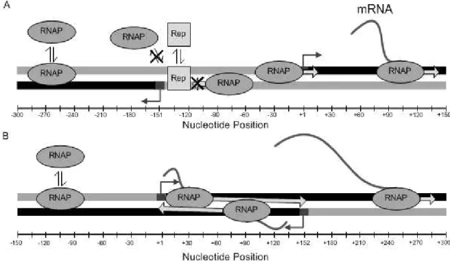
Figure 3.1 – Structure of (A) divergent promoters, and (B) convergent promoters, where

binding region is gray, elongation region is black and the angled arrows presents transcriptional

start sites (TSSs). Harpoons represent the binding and unbinding of RNAps and repressor

molecules, the x-axis represents the nucleotide position in relation to the TSS of the “right”

promoter. ... 15

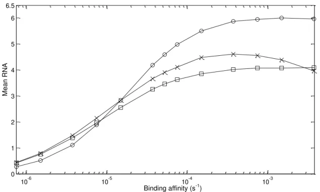
Figure 4.1 – Mean RNA numbers as a function of kbind rate. Here we represent (○) for

unidirectional promoters, (x) for divergent promoters and (□) for convergent promoters. ... 26

Figure 4.2 – CV2_{of the RNA numbers as a function of the binding affinity (k}

bind) rate over

time (at near-equilibrium). Here we represent (○) for unidirectional promoters, (x) for divergent

(18)

Page xviii

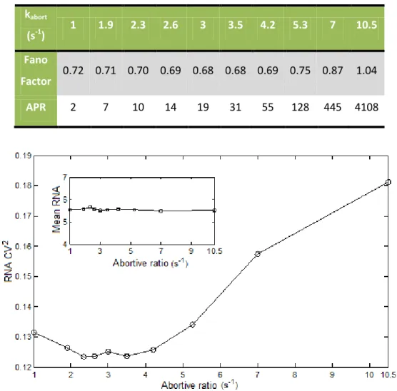
Figure 4.3 – The CV2_{of RNA production as a function of the abortive ratio (k}

abort). As can

be seen in the inset graphic we maintained the RNA number constant around 5.5 varying the

degradation rate. These simulations were all done on a divergent promoter with a distance of 200

nucleotides between the TSS. ... 29

Figure 4.4 – Time series of RNA production for the divergent case. ... 31

Figure 4.5 – Time series of RNA production for the convergent case. ... 31

Figure 4.6 – Time series of RNA production for the divergent overlap case. ... 32

Figure 4.7 – Probabilities for each nucleotide that an RNAp will bind to the DNA template of two divergent promoters. The binding region is located between both TSSs with 200 nucleotides between them. We tested three different values of kbind (standard value, 10 and 100 smaller values than the standard). ... 37

Figure 4.8 – Probabilities for each nucleotide that an RNAp will bind to the DNA template of two divergent promoters. The binding region is located between both TSSs with 200 nucleotides between them. For this simulation we set the rate constants so that they are no longer rate limiting of the RNAp movement along the DNA template. ... 38

Figure 4.9 – Probabilities for each nucleotide that an RNAp will bind to the DNA template of two divergent promoters. The binding region is located between both TSSs differing in number of nucleotides (N) between both TSSs. (A) N=100 (B) N=125 (C) N=150 (D) N=175 (E) N=200 (F) N=250 (G) N=300 (H) N=350 (I) N=400. In the y-axis we have the binding probability and in the x-axis we have the binding position. ... 39

Figure 4.10 – Probabilities for each nucleotide that an RNAp will bind to it, when binding to the promoter region. This simulation was done with convergent promoters with a binding region of 150 nucleotides and a distance between TSSs of 150 nucleotides. ... 40

Figure 4.11 – Probability distribution of time intervals between the productions of

consecutive RNAs on one side. The models vary in their distance between the TSSs (in

nucleotides) but all of them have a binding region of 200 nucleotides and were previously

(19)

x-axis is divided in bins of 3 s while the y-x-axis represents the probability that the production events

occurs within the bin duration. ... 42

Figure 4.12 – The Pearson correlation between sequences of choices of elongation

directions. All the models are the same as in figure 4.11. Here, Choice Lag does not have units,

since we use vectors of choices (0 for the “left” promoter and 1 for the “right” promoter”). ... 43

Figure 4.13 – Pearson correlation at lag 1 between the choices of directionality of

consecutive RNAs as a function of the distance between both TSSs for convergent (○) and

divergent (□) promoters. ... 46

Figure 4.14 –Mean RNA numbers in the (A) divergent (B) convergent promoters as a

function of the distance between the TSSs. In these models, both genes are identical and, thus, so

are their mean RNA levels. The standard kbindis represented in (□), kbind/ 10 is represented in (○)

and kbind / 100 is represented in ( ). ... 47

Figure 4.15 – Repression of unidirectional promoter at various steps of transcription

initiation. Y-axis is the repression factor and x-axis is the number of repressor molecules. The

repressed steps are, closed complex formation ( ), open complex formation (○) and is the promoter

escape (□). ... 52

Figure 4.16 – Correlation of RNA production in time at different lags for different

geometries: (○) divergent with 65 nucleotides between TSSs. The values in red correspond to the

correlation without repression and the values in black to the correlation with repression. ... 55

Figure 4.17 – Correlation of RNA production in time at different lags for different

geometries: (□) divergent with 150 nucleotides between TSSs. Values in red correspond to

correlation without repression and the values in black to correlation with repression, we also did a

divergent promoter (•) in the same arrangement but with two repressor binding sites where one

repressor site blocks the other and allows just one side to produce. ... 56

Figure 4.18 – Correlation of RNAp production in time at different lags for different

geometries: (x) convergent with 150 nucleotides between TSSs. The values in red correspond to

(20)

Page xx

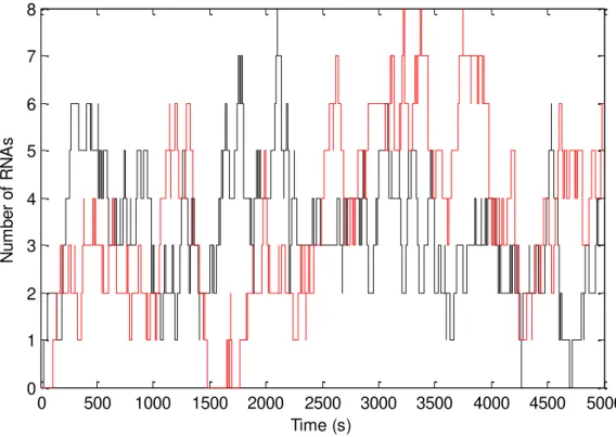
Figure 4.19 – Time series of RNA production for the convergent case (red and black line)

(21)

Table contents

Table 2.1 – Various values of as a function of the type of reaction. Taken from [33] .. 6

Table 3.1 - Chemical reactions, rate constants (in s-1), and time delays (in s) used to model

transcription initiation. ... 17

the steps that occur after the open complex formation. ... 18

repression and dissociation of repressor. ... 19

Table 4.1 - The Fano factor of RNA production for different arrangements as a function of

the isomerization rate. ... 28

Table 4.2 - Values of the Fano factor of RNA production and Abortive to Productive ratio

(APR) as a function of kabort parameter. ... 29

Table 4.3 - The mean and CV2_{of RNA production for different arrangements as a function}

of the isomerization rate. This rate was changed on the “right” promoter. Here kisom stands for the

standard isomerization rate used in this work: 0.095 s-1_{. ... 33}

Table 4.4 - The mean and CV2_{of RNA production for different arrangements as a function}

of the binding rate. This rate was changed in a particular region of the template. Here kbind stands

for the standard binding rate used in this work: 0.000075 s-1_{. ... 35}

Table 4.5 - The mean and the standard deviation of the time intervals between the

productions of consecutive RNAs from just one promoter. We joined the data obtained separately

for each promoter to have more samples. ... 41

Table 4.6 - The mean, CV2 and Fano Factor with the variation of the repressor size. For

these simulations we used two binding kinetics of the RNAp (the standard value and 100 smaller).

... 49

Table 4.7 - The mean, CV2 and Fano Factor with the variation of the dissociation kinetic

(22)

Page xxii

Table 4.8 - Repression of unidirectional promoter at various steps of transcription

initiation. Mean RNA levels as a function of the number of repressors present. ... 51

Table 4.9 - Repression mechanism for convergent arrangement with 150 nucleotides

between TSSs. Binding regions is consisted of 300 nucleotides. The repressor size is 21

nucleotides. ... 53

Table 4.10 - Repression mechanism for the divergent arrangement with 150 nucleotides

between TSSs. Binding regions is consisted of 300 nucleotides. The repressor size is 21

(23)

Chapter 1. Introduction

The objective of this work is to design a stochastic model of transcription initiation at the nucleotide level and use it to study the dynamics of RNA production in Escherichia coli (E. coli).

We study the dynamics between pairs of closely spaced promoters and also single unidirectional promoters for a comparison.

Cells are able to respond to environmental changes using regulatory mechanisms connected to their genetic circuits. This regulation often takes place at the stage of transcription initiation [1], which is the first step of transcription. Transcription is the process of synthesizing a Ribonucleic acid (RNA) transcript using the information contained in a determined region of the

Deoxyribonucleic acid (DNA). This process is executed by the RNA polymerase (RNAp) and is

present in both eukaryotes and prokaryotes, such as our model organism: E. coli.

The stochastic nature of gene expression leads to cell to cell variability in the number of RNA and protein molecules in monoclonal cell populations [2]. Fluctuations in the RNA and protein numbers over time have been observed at the single cell level [3, 4]. These fluctuations were detected in transcription using single-cell experiments [5] and have an important effect in the behavior of the cell.

Researchers have recently developed tools to model and simulate biological processes at the single event level using the stochastic simulation algorithm (SSA) [6]. These models [7, 8] have shown the ability to predict the statistics of such processes that have a stochastic nature, which would not be possible using deterministic kinetics.

The first stochastic model [7] of gene expression considered transcription to be an instantaneous process as a first approximation, but the execution of this process by the RNAp can take some time. To account for this, time delays were added to the model of transcription [9]. A delayed stochastic model of transcription at the single nucleotide level [8] was then proposed, which included dynamically pertinent events in elongation such as transcriptional pauses, error correction, arrests, premature termination and collisions between elongating RNAps. In that model transcription initiation was modeled as a delayed event whose duration followed a Gaussian distribution, to account for the rate-limiting steps inherent to this process [10].

In this work, using E. coli as a model organism, we follow the same strategy to model

(24)

Page 2

back to the open complex state. Also, it is noted that in this event the RNAp does not move but rather stays in the same position and “scrunches” the DNA [21, 22]. When the energy accumulated inside the RNAp is enough to break the promoter bond, the RNAp escapes the promoter and starts the elongation process.

Our model of transcription initiation at the nucleotide level, which includes all the reactions described earlier, has a great ability to study the dynamics of RNA production in promoters that are closely spaced, one event at a time. Further, we can use it to test the effects of varying the distance between transcription start sites (TSSs) or the influence of the directions of transcription of each promoter.

These closely spaced promoters can be organized with regard to the direction of transcription (which we will describe as “promoter arrangement”). In terms of arrangement, promoters can be tandem, convergent or divergent [1]. Closely spaced tandem promoters are oriented in the same direction, as they usually transcribe the same gene or operon. Convergent promoters are arranged in a face to face fashion and, thus, have a common region of elongation. Finally, divergent promoters have a common binding region for the RNAp and transcribe in opposite directions.

Closely spaced promoters have been found to be abundant in all simple organisms, ranging from viruses to chloroplasts and bacteria [23]. On the other hand, the eukaryotic genomes are generally less dense and less organized than prokaryotes, so the finding of such promoters in this organisms, as for example in the human PCNA locus [24], was less expected. It is now known that bidirectional promoters are also a common gene organization in higher order organisms, including humans [25, 26].

The use of a model at the nucleotide level enables the study transcription regulation at that level and the investigation of how the location of such regulators can affect the dynamics of RNA production [1, 27]. Using different transcription factor binding sites (TFBSs), it is possible to study the mechanisms of transcription regulation at various levels of transcription initiation [28]. Due to the interference between colliding RNAps we expect that closely spaced promoters have more complex gene expression patterns [29] and so can have a more complex regulation and so to understand such a complex system, using a detailed at a single nucleotide level is the best approach.

(25)

the kinetic constants of the rate limiting steps for both promoters independently, such as the open complex formation, in an independent fashion.

Using all this different parameters we investigated how asymmetric features affect the relative expression levels of both genes separately. To study the dynamics of RNA production, we characterized it in terms of mean and noise in RNA numbers, distribution of time intervals between consecutive production events, the correlation between choices of direction of consecutive elongation events and correlation between time series of RNA numbers.

In Figure 1.1 it is presented a scheme with the location where this work was done (TUT in Finland). This work was done in collaboration with the LBD group, who studies the dynamics of prokaryotic gene expression and gene regulatory network. This work appeared because in previous models, transcription initiation was modeled as a single delayed event.

Figure 1.1 – Scheme with the objectives of this work (left side), the motivation behind this work (right side) and the location where this work was done (green box).

(26)

(27)

Chapter 2. Theoretical framework

In this chapter we give a theoretical description of the framework behind the main topics of this work. Particularly we give some insights on how stochastic simulations appeared and evolved throughout the years and why this type of simulations is considered to be very useful in studies of biological processes such as gene expression. Then we describe the steps involved in transcription initiation, including a structural description of the existing RNAps and their interactions with the DNA during these steps. Finally we also have a topic on closely spaced promoters and how they can be organized in different arrangements and their influence in gene regulatory mechanisms.

2.1. Stochastic Simulation Algorithm

Modelling is an approach to characterize the state of the elements inside a system and the interactions between those elements. Models using the present knowledge of a system can help in testing if our understanding of that particular system match the data obtained in experimental procedures.

From the point of view of classical mechanics, systems of chemical reactions are considered as deterministic, because it is possible to predict the evolution of the system. The deterministic approach has slight problems in explaining such processes that have a stochastic nature, for example gene expression and their regulatory mechanism [3, 4, 5]. Thanks to the impossibility of calculating the exact moment that an event takes place, although we can estimate that probability.

Solving a system of coupled ordinary differential equations (ODEs) is the most conventional way of describing and simulating (using the deterministic approach) the behavior of molecules reacting in a homogeneous and thermally equilibrated mixture. This system has one equation for each of N active chemical species in the volume, where each equation describe

changing rate of the concentration Xi of each chemical species Si taking in consideration the

concentration of the other species, stoichiometry and reaction constants of the R channels through which they interact. This set of equations forms the reaction rate equation (RRE) [30]:

∑ ( )

(2.1)

Here is the vector that describes the stoichiometry of reaction and is considered as

the mean ‘rate’ at which the same reaction occurs as a function of the vector of the current

(28)

Page 6

As stated before, some biological systems have a stochastic nature and so due to this reason a new approach is needed. The stochastic approach instead of calculating the exact moment that an event takes place, it is involved in estimating the probability

₍

)

of having the given

concentration

in the reaction volume at time

after the initial

concentrations of all the

molecules and the initial time of reactions:

and

respectively. Using the probability that the molecules in the volume at time t react in the next infinitesimal time interval (t+dt) via

reaction , which is defined as the propensity function or ( ).

The stochastic approach can be expressed as a partial-differential equation also known as the chemical master equation (CME) [31], which is also known as the Kolmogorov forward equation for a stochastic kinetic process [32]:

( )

∑

[

(

) (

|

)

( ) (

)]

(2.1)

Here also corresponds to the absolute number of all the reactants that change when the reaction occurs.

This propensity function can be written as _{( )} _{( )} , where _{( )} is the number of possible reactant combinations in the reaction volume and is a kinetic constant such that gives the probability that in the next infinitesimal time dt a determined molecule will spontaneously

react via . Different types of reactions can have different _{( )} as can be seen in table 2.1.

Table 2.1 – Various values of _{( )} as a function of the type of reaction. Taken from [33]

Type of reactions ( )

→ 1

→

→ ( )

∑ ( )

→ _{∏ ∏}( )

(29)

is way analytical simulators started to be more utilized. The Stochastic Simulation Algorithm (SSA) [34] is a Monte Carlo method that simulates numerically the time evolution of well stirred reaction systems. The time goes forward in discrete steps and in each step a reaction is explicitly executed and the effect on the number of each molecule is settled. Probability distributions are used to determine the time of the next reaction.

The SSA produces in a single run one of the possible exact temporal trajectories of the CME and can be represented by the following steps:

1. Initialization: Define R reactions rates (k1,…,kR) and the initial molecule number

( 1,…, N) and then set time t = 0 and reaction counter n=0.

2. Calculate R propensities using the current population of molecules, p1=k1•h1,…,

pR=kR•hR where h is the number of all possible distinct molecular interactions in the

current state(see table 2.1 for different types of h). Calculate ∑ and store all

the propensity values.

3. Calculate the pair (τ, µ) using two random numbers r1 and r2 (from a U(0,1) uniform

distribution, using ( ⁄ ) ( ⁄ ) and µ has to satisfy the following: ∑ ∑

4. Calculate the actual value of t using the pair (τ, µ) and adjust the reaction counter by one.

a. If t + τ ≥ tstop , end the simulation.

b. If t + τ < tstopthen set t = t + τ, and update the molecular numbers according to

the type of reaction that occurred using .

5. Go back to step 2.

Note that the procedure in step 3 is done by one of the original formulations of the SSA, the Direct Method [34] which is computationally less intensive then the other formulation: the First Reaction Method. For large systems, these methods can be computationally heavy and so other methods started to appear in order to that improve the computational performance without affecting its exactness, and so the Next Reaction Method [35] and the Logarithmic Direct Method [36] were proposed. The First Family Method [30] is a generalization of the above methods and has the advantage of being able to choose either the Direct Method or the First Reaction Method on step 3 of the SSA based on the total propensities of the reactions (which are grouped into “families”).

Finally as previously described, the need to account with the duration of processes that take non-negligible to complete, such as transcription, led to the modification of the SSA [35], where time delays started to be added to account for those durations. These delays can be implemented

(30)

Page 8

The delayed SSA was used to model transcription at the nucleotide level [9] and was shown to match [37] the dynamics of RNA and protein production at the single RNA and protein level [38, 39].

2.2. RNA polymerase and the execution of transcription initiation

Transcription initiation is the first step in transcription and is executed by an important enzyme: the RNAp. Due to this, the structure of the RNAp and how that structure affects its function in the transcription process is an important feature to understand in this process.

Different organisms have different types of RNAps, which can be divided into single-unit multi-subunit RNAps. The single-unit RNAp is normally associated to virus and one of the most studied examples of this type comes from the T7 bacteriophage RNAp. Multi-subunit RNAps are associated to eukaryotes, bacteria and archaea, although there are major differences in the RNAps within those domains, even though there is evidence of a correspondence between structure and function of various subunits found in archaea and eukaryotes compared to bacteria [40, 41]. In this case, one of the most studied examples comes from the E. coli RNAp.

Both the T7 and E. coli RNAp have been the focus of single-cell studies both structurally

and functionally. The core structure of the E. coli RNAp (formed by five subunits: two α, β, β’ and

ω) and its relevance to transcription initiation were studied at a resolution of 15 Å using cryo-electron microscopy and image processing of helical crystals [42].

Other bacterial organisms have been used to gather information on E. coli RNAp using

higher resolutions, such as the Thermus aquaticus [43, 44] or the Thermus thermophilus [45]. On

the other hand T7 structure has been studied at a resolution of 3.3 Å [46] and despite the structural differences, evidence of a similar functional mechanism of the RNAp was found in both organisms using structural and functional studies [47, 48, 49], making T7 RNAp also suitable for mechanistic comparisons with the E. coli RNAp in the process of transcription.

Transcription initiation in bacteria starts with the localization of the promoter-specific region (also known as promoter search) [11, 12, 13, 14], which in bacteria requires the binding a

polypeptide (called σ factor) [50] to the core enzyme, forming the holoenzyme, reducing the affinity of the RNAp for nonspecific DNA and increasing the affinity to various promoters. T7

RNAp also locates promoters using a similar mechanism but doesn’t need the binding of additional

polypeptides due to its high affinity to specific T7 promoters [51].

The housekeeping sigma factor (σ70_{), which is considered to be the most important}_σ

(31)

and thymine, upstream of the -35 element (that is normally addressed as the “UP element”) [52] .

The “UP” element is recognized by both α subunits [53].

Other σ factors, which are normally related to genes that respond to stress situations like UV radiation or heat shock, recognize less common promoter motifs, as they are only needed in special conditions [50]. In figure 2.1 we show the interaction between the various subunits of RNAp and the promoter motifs.

Figure 2.1 – The interaction between the subunits of RNAp and the core promoter. The consensus sequences for the -10 and -35 promoter motifs and the “UP element” are also shown. The contacts between RNAp and the promoter are shown in solid lines. Figure taken from [54].

Eukaryotes have several types of RNAps, depending on the type of the synthesized RNA. The RNAp II is the most studied one and as other eukaryotic RNAps, RNAp II alone doesn’t

recognize the eukaryotic promoter motifs, namely, TATA box, CCAAT-box and GC-box and others [55]. Due to this the binding of initiation factors is required before transcription initiation starts, which leads to a high level of control over transcription [56]. This control is also associated with the binding of other accessory factors, transcriptional activators and co-activators that regulate the rate of RNA production from each gene in response to different conditions [56]. Since in this paper we focus on bacterial transcription initiation, we will not enter into a detailed vision of the eukaryotic mechanisms.

The localization of the promoter in prokaryotes results in conformational changes in the DNA and the RNAp, which leads to the formation of a closed complex (RPc). These changes

include the DNA bending to wrap of upstream DNA and loading the downstream DNA in the active site of the RNAp [57, 58]. This mechanism proceeds with the RNAp loading of the template and non-template DNA positioned at the TSS, the unwinding of the double stranded DNA, the assembly and tightening of the RNAp clamp [58]. This stage is called isomerization and can be simplified into just one single isomerized complex (RPi). This step can also be considered a rate

(32)

Page 10

[15]. A real-characterization of these isomers in the T7A1 promoter, using E. coli RNAP [59]

showed that the transition between the various intermediates is very fast, supporting this simplification. This mechanism finally proceeds with the formation of the open complex (RPo).

Before starting elongation and escaping the promoter (which is the last step of transcription initiation) the initial transcribing complex (ITC) is involved in a repetitive cycling of the RNAp back to the open complex, and releasing short abortive RNA transcripts (that normally range from 2 to 16 nucleotides, but sometimes it is observed aborted transcripts up to 20 nucleotides) [60, 61], this process is called abortive initiation. Recent studies showed this process is involves a

“Scrunching” mechanism [21, 22], where the RNAp doesn´t move forward, but “scrunches” the

downstream duplex DNA in a through formed by subunit β′ and enclosed on top by the subunit β.

This process accumulates energy, necessary to break the bond between the RNAp and the promoter leading the RNAp to escape the promoter and turning into an elongation complex (EC), capable of producing a full RNA transcript after termination of the transcription and the promoter available to receive another RNAp and starting the initiation process all over again.

In a recent study [62], abortive initiation was also detected in vivo using the bacteriophage

T5 N25 promoter using the E. coli RNAP, which was an important find because until that, this

process was only observable in vitro.

Note that the sigma factor has also an important role in abortive initiation [63], so after the RNAp starts elongating, the σ factor is released stochastically [64] and can bind to other RNAps helping in the location of other promoters (defined as the σ cycle). Mooney and colleagues found that sometimes the sigma factor is not released until termination and that it can be used as an elongation regulator [65]. We decided to not include specifically the σ action into our model due to the complexity associated with using all the different observations of the previous models.

To model transcription initiation we need not only spatial information about the process, but also temporal. The duration of some of the steps previously described can vary widely between different promoters [11], even when their sequences only differ by one or two nucleotides [66]. It has also been studied that for example just one change in the nucleotides base in the spacer region between both promoter motifs can also change dramatically the promoter activity [67]. For example the abortive initiation and promoter escape durations are dependent on the promoter interactions (and in this case, the stronger the promoter the slower is this process) but can also vary due to small changes in the downstream region (initial transcribing sequence) [60, 61]. Temperature can also affect the duration of these steps [15, 68] as well as the concentration of Mg2+

[68, 69] or the concentration of K+ _[68].

(33)

Figure 2.2 –The RNAp can bind nonspecifically to DNA and searches for the promoter. The σ70

subunit recognizes to the -35 and -10 promoter motifs and forms a closed-promoter complex. The RNAp then unwinds DNA around the initiation site forming an open complex. Then transcription is initiated followed by the release of sigma and the elongation of the RNA chain. Figure taken from [70].

We note that in figure 2.2 the “UP element” and its interaction with subunits α (which we note that some promoters actually don’t have) is not represented and also some steps of transcription initiation like the abortive initiation are not included.

2.3. Closely spaced promoters and regulation mechanisms

In the previous section we talked about how transcription initiation starts with the localization of promoters and how the interaction between the RNAp and those promoters affect this process. In this section we will emphasize on the actual location of such promoters in the DNA template, as this location can also play an important role in regulatory mechanisms [1].

The compilation of several promoters in E. coli [71, 72] led to an organization of closely

(34)

Page 12

in two different directions. In figure 2.3 we exhibit the three possible arrangements of closely spaced promoters. Note that in some cases, the promoters P1 and P2 can be overlapped.

Figure 2.3 – Possible types of closely spaced promoter arrangements. There are three types of arrangements: tandem (A), divergent (B), convergent (C) promoters.

The first divergent promoters to be discovered were the promoters PR and PRM, in the

lambda bacteriophage (λ phage) [73]. These promoters are one of the most studied cases of gene regulatory network [74, 75] and since the in the decision between two different paths in this network involves a random process, they were also the reason why stochastic models started to be used in such studies [7]. The studies in λ phage lead to the discovery of other divergent promoters

present in E. coli, for example the arginine gene (argE and argCBH promoters) [76] or the PC and

PBAD promoters of the L-arabinose operon, which have been extensively studied by Schleif and

colleagues for more than 30 years [77, 78].

A compilation of closely spaced promoters found several promoters in various simple organisms such as bacteria and their viruses (for example the phages), mitochondria, chloroplasts and viruses of eukaryotes [23] showed that these types of promoters represent a general type of gene organization in this type of organisms. We should mention that Beck and colleague [23] used a different notation for the promoter arrangement, as they address the convergent arrangement as

“face-to-face” promoters and divides the divergent promoters into “back-to-back” and “overlapping” promoters.

With the completion of the genome sequencing in E. coli K-12 (one of the most used

strains) [79] most promoters and their functions were identified. The location of such promoters have a regulatory role in transcription, as a recent statistical analysis [80] revealed that both operons that regulate each other and operons that are co regulated tend to be in close distance of each other and showed a tendency of divergent promoters in this type of regulation.

(35)

distance of 118 bp between genes, the genome is made mostly of coding DNA. The human gene, which is less dense then the E. coli genome, contains a 2.9 Gbp sequence with an estimation of

around 39000 genes [81]. This means that for a mean spacing of around 75 kbp for each human gene there is an average gene size of 27 kbp.

This implies that there is a large amount of noncoding DNA present in the sequence. Since the eukaryotic genome isn’t considered to be as organized as in bacteria, it was a surprising discovery when Adachi and Lieber identified bidirectional genes in the human chromosomes 21 and 22 [25]. A subsequent study [26] showed a prevalence of bidirectional genes in the human genome and among mouse orthologs, which means that this prevalence is often conserved along the species evolution.

We should notice again, that another notation for the promoter arrangement was used by Adachi and Lieber [25]. They address tandem orientation as “head-to-tail”, convergent as “tail

-to-tail” and divergent as “head-to-head”. To avoid the confusion of having various notations, we

decided to use the “tandem, convergent and divergent” notation in the rest of the work, and also use divergent overlap, when the distance between TSS only allows one RNAp to transcribe at a given time, which we consider to be of 110 or less nucleotides This is because we consider the size of the RNAp as 55 nucleotides when in diffusion process (note that we use a different size for elongation, which will be focused on more detail in the model section) based on footprint studies [52, 82, 83, 84, 85], where the RNAp protects around 50 to 60 nucleotides of the DNA template in the upstream region (there is also a protection of the downstream region with the opening of the DNA strand leading to the open complex formation).

In this thesis we focus on E. coli bidirectional promoters, considering both the divergent

and convergent arrangements, hence we extracted 897 known and 4010 predicted promoters (specifically recognized by σ70_)in_{E. coli}_{from RegulonDB database (version 7.0) [86].}

From the predicted promoters, there were several promoters of the same gene so we counted only the first promoter (p1 in the database) of each gene to avoid repetition of the same genes. From this, 1671 predicted promoters were extracted for this study, for a total of 2568 promoters. Using this number of promoter we found 258 pairs of divergent promoters and 186 pairs of convergent promoters with a distance between their TSSs lower than 800 nucleotides.

The distributions of nucleotide distance between the TSSs for both geometries are shown in figure 2.4. We observe that the bulk of the distribution of distance between adjacent TSSs is below 200 nucleotides (88.8% for convergent and 61.8% for divergent). The mean distance (in nucleotides) for convergent is 108.4 and 225.7 for divergent, therefore, this range of was used as a reference for our models.

(36)

Page 14

Figure 2.4 – Numbers of promoters pairs with a given number of nucleotides between the TSSs for (A) divergent promoters, and (B) convergent promoters. Gray bars are used for the known promoters and black bars are used for the predicted promoters.

This type of promoters can also be classified depending on the function of the gene products. Beck and colleague [23] classifies them as S-S if both transcripts determine structural polypeptides, R-S if one transcript determines a regulatory molecule and the other a structural polypeptide, or R-R where both transcripts determine regulatory molecules. These regulatory mechanisms [27] can be positive (activation), negative (repression), or depending on the circumstance can be of both types.

In this work we focus on repression mechanisms, as repressing the gene expression at the transcription level is probably the most used method of controlling the RNA production. Steric occlusion is probably the most common and simple method of repression, as in this method the repression molecule binds to the DNA and prevents the RNAp to start transcription [87, 88]. This repression can prevent specific steps in transcription depending on their TFBSs and size (such as the binding to the promoter, the transition from closed to open complex, or the promoter escape) [28].

It has been shown that the most common TFBS position is near the TSS (both in downstream and upstream regions) [88]. Our model allows us to choose the TFBS location and repressor size to be able to study the effect of repressor location and repression of specific steps, not only in single promoters but also in bidirectional promoters. Multiple TFBSs on the same DNA template are also allowed.

0 100 200 300 400 500 600 700 800 0 5 10 15 20 25 30 35 40

Nucleotides between TSSs

N u m b e r o f P ro m o te rs

0 100 200 300 400 500 600 700 800 0 5 10 15 20 25 30 35

Nucleotides between TSSs

(37)

Chapter 3. Materials and Methods

In this section we present the description of the reactions used to create our model, the respective kinetic rate constants and delays. The calculations used to characterize RNA production is also presented in this section.

3.1. Creating the model

Modeling transcription initiation traditionally consist of three overall steps: binding of RNAp to promoter, open complex formation and the promoter escape [1]. Some of those steps present in that type of model are undoubtedly oversimplified as the numerous small steps involved in each of them are integrated into single reaction.

We use the proposed strategy [9] to model the dynamics of transcription initiation in bidirectional genes, considering both convergent and divergent promoters [1]. In figure 3.1 we show two model representations of bidirectional promoters and some of the reactions that used in this model. Locations within the promoter region are designated by the position relative to the TSS at the right side. The position of this TSS is set to be +1, positions to the left are negative and to the right are positive (note that by convention in Biology the first upstream nucleotide before the TSS is at position -1 and the TSS is the position +1, meaning that there is no position 0).

(38)

Page 16

In figure 3.1 the regions of elongation (which the RNAp can also percolate by diffusion) are represented in black, while regions where only diffusion can take place are represented in gray. Elongating RNAps are represented with an elongating RNA chain, which are not present in diffusing RNAps. RNAps bound to the DNA template have an arrow that represents the current direction of movement.

If a repressor is bound to the DNA template (at the TFBS), it blocks the movement of both diffusing and elongating RNAps. In figure 3.1 (A) the TFBS is represented between position -140 and -120 on the template. A bound repressor also prevents the binding of RNAps to that region, and that region alone. This repression is represented using a cross over the movement arrows of the RNAp.

In figure 3.1 (A), it is illustrated two divergent promoters, whose TSSs are located at -151 and +1. The “left” gene can only be transcribed by RNAps diffusing in that direction and the gene to the right can only be transcribed by RNAps diffusing to the corresponding direction. In figure 3.1 (B) it is illustrated two convergent promoters, whose TSSs are located at +152 and +1 and also differs from figure 3.1 (A) since it contains an overlapping elongation region. . The elongating RNAp removes the diffusing RNAps and RNAps bound to TSS. In case of two elongating RNAps colliding in the overlapped region, either one of them randomly dissociates or both dissociate.

The reactions, the standard rate constants and delays used to model transcription initiation are presented in table 3.1. In this table we present the binding and unbinding of the RNAp to the DNA template, the search for the promoter using linear diffusion, the closed and open complex formation, isomerization, and collisions between diffusing RNAps.

Note that in the reactions presented in tables 3.1, 3.2 and 3.3 we don’t express specifically the differences between different promoters present in our model. This means that we don´t specify if the reactions are from the left or the right side (see figure 3.1) or even if they are from convergent or from divergent promoters. The only difference between these situations will be on the indexes, so because of this we decided to only include one reaction for each event, which is much clearer.

Most reactions in the model are instantaneous, that is, once the two reacting molecules meet and react, the product is produced instantaneously and its amount updated. Instantaneous

(39)

Some reactions need to account for the time that the processes take to occur, once initiated.

Such delays in the release of products are exemplified as follows: → ( ) . When this reaction occurs, molecule C is placed on a waitlist and is only made available for reactions, after 

seconds have elapsed. We can generate  randomly from any desired distribution each time the reaction is chosen to occur. Such delayed events are only introduced when the time that the process takes to occur is sufficiently long to affect the kinetics of the system. Substrates that are not consumed in the reaction are indicated with (*).

transcription initiation.

Identifier Reaction Rate constants

and delays Ref.

(1) b

D D

k

[n-Δ , n+Δ ] n

RNAp + U



O

kb = 0.000075 [12]

(2) f

D D]

k

[n-Δ , n+Δ

n

O



RNAp + U

kf = 0.3 [12]

(3) m

D D

n+Δ +1 n-Δ

n+ U k n+1+ U

O





O

km = 660 [12]

(4)

D

c

TSS+Δ

k

c

O





RP

kc = 0.5 [12]

(5) RP + U_c _{[TSS+1, TSS+19]} ki RP_i ki = 0.095 [15]

(6) o

i k o

RP



RP ko = 2 [15]

(7) D

D D

n+2Δ 1 n

[n-Δ , n+Δ ]

*O + O

U + RNAp

m

k

 

km = 660 [12, 101]

In the reactions presented in table 3.1 RNAp stands for the RNA polymerase, Un stand for

the nth unoccupied nucleotide. Ranges of nucleotides are denoted such as U[start, end], denoting a

stretch of unoccupied nucleotides from indexes start to end. As reported in footprint studies [52,

82, 83, 84, 85] the bound RNAp protects around 50 nucleotides on the template. In our model each RNAp occupies 55 nucleotides, and we name it as On, to account only for the active center (this

means that the diffusing RNAp is occupying the range [n-ΔD, n+ΔD], where ΔD = 27). Here RPc,

RPi and RPo correspond respectively to the closed complex, the isomerization complex and the

(40)

Page 18

The reactions used to model the steps that occur after the open complex formation, such as the abortive initiation, promoter clearance, the initial transcribing complex, the elongation complex formation and the collision between the elongation complexes and different RNAps at various steps is presented in table 3.2.

Table 3.2 - Chemical reactions, rate constants (in s-1), and time delays (in s) used to model the steps

that occur after the open complex formation.

(8) E

D

2Δ 1 n

[ Δ , Δ ]

*E + O

U RNAp m D n n n k     

 km = 660 [12, 101]

(9)

el E

E E

n+2Δ +1 n

[n-Δ , n+Δ ]

k

*E + E

U + RNAp



kel = 42 [101]

(10)

el

E D

el

E D

TSS-Δ c [TSS, TSS-2Δ ]

TSS i o TSS-12

[TSS+Δ , TSS-2Δ ]

k

*E + RP U

k *E + RP /RP /E

U



 kel = 42 [101]

(11) el

o k TSS

RP E kel =42 [21, 22, 61]

(12) el/4

TSS+n k TSS+n+1

E E kel = 42

n≤12 [21, 22, 61]

(13) _E_TSS+n ka _RP_o ka = 4.2 [21, 22, 61]

(14)

el E

D TSS+12 TSS+Δ 12

TSS+13 [TSS+12, TSS+2Δ +12]

k

E

+U

E

+U







_k

el = 42 [21, 22, 61]

(15) el

E E

n n+Δ

k

n+1 n-Δ

E +U





E

+U

kel = 42

n≥13 [100]

(16)

el last

last E last

n

el el [n -2Δ , n ]

k

E

RNA(

τ ) + RNAp(τ ) + U





kel = 42

el ~ G(k, 1/kel)

[100]

(17)

_RNA

_

kd k_d = 0.006 [105]

In the reactions presented in table 3.2, the Ribonucleic acid is designed as RNA for and En

(41)

to 23 nucleotides [83], we decided to use 25 nucleotides as it is also reported by [89], so because of this it occupies the range [n-ΔE, n+ ΔE], where ΔE=12.

The reactions used for repression mechanism, as the mechanism of transcription regulation used for this model is presented in table 3.3.

repression and dissociation of repressor.

(18) r

rep rep

[n-Δ , n+Δ ]

k

n

Rep + U



R

kr = 0.0167 [113]

(19)

R

_n



ku

Rep + U

_[n-_{Δ , n+Δ ]}_rep _rep ku = 0.004 [113]

In the reactions presented in table 3.3, a repressor not bound to the DNA template is designed as Rep and the repressor bound to the DNA template is designed as Rn and occupies the

range [n-Δrep, n+Δrep]. Each different repressor molecule can occupy a different number of

nucleotides. In this work we use a standard value of Δrep = 10 as it is the value for the principal

binding site of the lac repressor [87], which is one of the most studied repressors in E. coli, and it is

also close to other repressor footprints measured in E. coli [90]. We also varied the values of

repressor size to study its effects in transcription regulation.

A description of the specific reactions used in our model is given below (using the respective identifiers from tables 3.1, 3.2 and 3.3). Parameter values used in the reactions were obtained from measurements in E. coli, directly or indirectly from the respective references

column.

Once the RNAp binds to the template via reaction (1) it diffuses linearly (also known as

“sliding”) [12, 91] on the DNA template (3). We point out that the binding of RNAp happens to one strand at a time thus the direction chosen by the RNAp can´t change during the sliding unless the RNAp unbinds. We didn´t include the three-dimensional diffusion in solution and intersegment transfer [92] as they are mostly means to make long transfers in the DNA template. If the RNAp is blocked by another RNAp or by a repressor, and doesn´t find a TSS, the RNAp eventually dissociates from the DNA strand (2) [12]. In our simulations we used a value for the initial concentration of free RNAp to be 28 molecules per cell [93].

(42)

Page 20

We note that when referring to closed complex formation, we define it as the conformational changes that occurs after the finding of the TSS [12, 14], and not as all steps including finding of the promoter and diffusion [1].

As stated before, because of the size occupied by the RNAp, we consider promoters with a distance between TSS of 110 or less as divergent overlap so we consider that for this case, only one RNAp can transcribe at a given time and that once it starts transcription in one direction it cannot be redirected to the other direction [94]. We point out that we don’t consider special cases that

have been studied in λ phage [95], where the interference between the occupancy of an RNAp at one of the promoters (PR) and the other promoter (PRM) was studied. It was found that for a very

specific distance between the TSSs this interference was greatly diminished, allowing RNAps at both promoter sites to start transcription at the same time.

The next step in this process is isomerization (5), where the RNAp structure changes, and occupies around 20 more nucleotides (from +1 to +20) as reported by DNA footprints [82, 83, 84, 85] and finally the formation of the open complex is done (6). At this step the RNAp occupies around 75 nucleotides (from -55 to +20).

We didn’t included the reverse reactions in the open complex formation because on strong

promoters, open complexes are much more energetically favorable, and the transition from closed to open complex is essentially irreversible [85], but we point out that these reactions can be easily added to our model if we actually needed. There are also other models of transcription initiation that don´t use the reverse reactions after the formation of the closed complex [96]

Following the formation of the ITC via reaction (11), the RNAp doesn´t move forward, but

“scrunches” the DNA (12) [21, 22]. This process continues until the energy inside the RNAp is enough for it to be able to break the bonds with the promoter (14). We added the abortive path (13) which competes with the scrunching path (12), returning to the state of open complex.

A model of the abortive initiation step in transcription initiation steps, which includes the abortive path, scrunching path but also an escape path was proposed by Xue and colleagues [97]. This is a detailed model, where for every different path at different positions have specific kinetic parameters. Unfortunately the kinetic parameters were calculated for T5N25 and T7A1 (bacteriophage) promoters, which are considered to be much faster initiators then for example the

lacUV5 promoters [18] even though the interaction with such different promoters share similar

mechanisms in the abortive initiation [19]. For simplicity we used the same kinetic parameters at every nucleotide and we only allow the escape after the scrunching of the 12th nucleotide.

Note that in this model we don´t include a path for unproductive ITC´s, where the RNAp escapes the promoter very slowly, if at all. This process was observed in few cases, thus it doesn’t

(43)

We tested an abortive rate ranging from 1 to 10.5 s-1_{and decided to use 4.2 s}-1_{as our}

standard value, which have a value of Abortive to Productive (APR) ratio that was within the values reported in abortive initiation studies [61]. With this value, the promoter can also be considered a rate limiting step (as it takes an average of 20 s for the RNAp to escape the promoter). This complies with observations made with the lacUV5 promoter [15, 99]. These results are presented in Chapter 4, section 4.2.

Note that as soon as the RNAp escapes the promoters and starts the elongation (15), another free RNAps in the cell may occupy that promoter and start a new cycle of transcription initiation.

We add a final reaction for the elongation (16), where the elongation complex exits our region of interest. We add a delay for the release of the RNAp and the mRNA using a Gamma Distribution (the function G in the reaction), where k equals to the number nucleotides that still

needs to be elongated the respective gene and θ equals to 1/42 s (coming from the elongation rate) [100].

Considering that we wanted to mainly study the effects of the transcription initiation on the production of RNA and since interference is done in our zone of interest, normally we use a value of k equal to 150 nucleotides. This means that the elongation region is normally the same as the binding region, but we sometimes change this value to account for the increase in the binding region. We point out that since the elongation rate is so high, that changes up to 200 nucleotides, just makes an average increase of 5 s to the production time.

We include in our model collisions between ECs (9), where one of the two colliding RNAps is released from the template (randomly chosen among the two), or both of them are released from the template.

We also use the same system as in (9) to model collisions between 2 diffusing RNAps (7), where one of the RNAps or both of them randomly dissociates from the template.

In convergent promoters, it is possible for elongating and diffusing RNAps (8) to collide, and since the binding between an elongating RNAp and the template is so strong that it can remove a complex at a promoter [101], these can force, when collisions occur, diffusing RNAps, which have a weaker binding affinity then complexes at a promoter [102]. This means that the EC remains in the template and the diffusing RNAp dissociates from the template.

We also add the “Sitting duck” mechanism as reported by [101] where an EC collide with promoter complexes (closed, isomerization, open or ITC) at a converging promoter (10). Degradation of mRNA via reaction (17) is modeled as a single step reaction.

Orientador: José Manuel Fonseca, Professor Auxiliar, FCT-UNL Co-orientador: André Sanches Ribeiro, Professor Assistente, TUT, Finlândia

Leonardo Pedro Donas

-

Boto de Vilhena Martins

STOCHASTIC MODEL OF

TRANSCRIPTION INITIATION OF

CLOSELY SPACED PROMOTERS IN

ESCHERICHIA COLI

Orientador: José Manuel Fonseca, Professor Auxiliar, FCT-UNL

Co-orientador: André Sanches Ribeiro, Professor Assistente, TUT, Finlândia

Resumo

Abstract

Acknowledgements

Abbreviations and Symbols

Contents

Figure contents

Table contents

Chapter 1.

Introduction

Chapter 2.

Theoretical framework

2.1.

Stochastic Simulation Algorithm

(

)

of having the given

concentration

in the reaction volume at time

after the initial

and

∑

[

(

) (

|

)

( ) (

)]

2.2.

RNA polymerase and the execution of transcription initiation

2.3.

Closely spaced promoters and regulation mechanisms

Chapter 3.

Materials and Methods

3.1.

Creating the model

RNAp + U

O

O

RNAp + U

O





O

k

O





RP



k

E

+U

E

+U





k

E +U





E

+U

k

E

RNA(

τ ) + RNAp(τ ) + U





RNA

₍

_RNA

_