Energy Consumption of Functional Programs in the Context of Lazy Evaluation

(1)

UNIVERSIDADE DA BEIRA INTERIOR

Engenharia

Energy Consumption of Functional Programs in the

Context of Lazy Evaluation

Gilberto Amaral Cordeiro Melfe

Tese para obtenção do Grau de Mestre em

Engenharia Informática

(2º ciclo de estudos)

Orientador: Professor Doutor Simão Melo de Sousa

Co-orientadores: Professores Doutores João Paulo Fernandes, Fernando Castor

(2)

(3)

Dedication

To all that contributed...

(4)

(5)

Acknowledgments

I would like to thank to all that have, directly or indirectly, helped with the development of this work. In particular I would like to thank my adviser, for the extreme availability, and patience, to listen to all my doubts/problems related to this work, and unrelated to the work. Without him I would never have finished this work. A word of appreciation goes also to the co-advisers, brazillian colleagues co-authors of a conference paper (Luís, Francisco, Paulo) and all colleagues at the Release Group who kindly welcomed me into their laboratory.

(6)

(7)

Resumo

O planeta Terra dispõe de recursos naturais limitados disponíveis para suportar o nosso quotid-iano, sejam eles matérias primas para manufactura ou energia para gerar trabalho. O ritmo a que consumimos esse recursos está a aproximar-se dos limites dentro dos quais a natureza pode restabelecê-los, e a que nós podemos extraí-los.

É com esses recursos que desenvolvemos a mais variada tecnologia, da qual o nosso modo de vida moderno é cada vez mais dependente, para providenciar todos os tipos de serviços imagináveis. Em particular, as Tecnologias de Informação e Comunicação (TIC) são uma parte essencial da vida de hoje. Com cada vez mais dispositivos, suportando diferentes serviços, em utilização, o seu consumo de energia cresce diariamente.

Cientes deste factos, os desenvolvedores de hardware/software procuram modos de optimizar o consumo de energia dos artefactos computationais (hardware/software).

O nosso trabalho, focado no software, foi motivado pela necessidade de apurar se, e até que ponto, podemos poupar energia adaptando programas existentes.

Nessa medida, implementámos um benchmark que foi utilizado para analisar o consumo en-ergético de várias implementações de abstracções de estruturas de dados comuns, implemen-tadas na bibliotecaEdison, para a linguagem de programaçãoHaskell.

As nossas descobertas levam-nos a concluir que podemos poupar energia, extensivamente, de-pendendo do padrão de utilização, por parte dos programas, das operações nativas disponíveis naEdison.

Palavras-chave

Eficiência energética, Estruturas de dados puramente funcionais, Edison, Haskell

(8)

(9)

Resumo alargado

A sociedade moderna tem evoluído a um ritmo admirável. O nosso estilo de vida moderno, faz cada vez mais uso de tecnologias de toda a espécie para nos facilitar a vida. Como exemplos temos, a conectividade global, providenciada pela Internet, a facilidade de viajar por todo o mundo, etc.. Esse mesmo, desejado, estilo de vida leva-nos a querer consumir mais produtos e serviços.

No entanto, temos recursos naturais limitados disponíveis para suportar o nosso quotidiano, sejam eles matérias primas para manufactura ou energia para gerar trabalho. Por outro lado, o ritmo a que consumimos esse recursos está a aproximar-se dos limites dentro dos quais a natureza pode restaurá-los, e a que nós podemos extraí-los.

Em particular, as Tecnologias de Informação e Comunicação (TIC) são uma parte essencial da vida de hoje. De modo crescente, as nossas actividades diárias fazem uso de todo o tipo de dispositivos como smartphones ou outros “computadores”. Com cada vez mais dispositivos, suportando diferentes serviços, em utilização, o seu consumo de energia cresce diariamente. Esta realidade verifica-se por exemplo no crescente consumo energético do largo número de data centers que suportam serviços online.

No contexto das TIC a preocupação em/necessidade de, utilizar os recursos criteriosamente é reconhecida à bastante tempo, tendo tido o foco primeiramente no hardware, e mais re-centemente no software. Os desenvolvedores de hardware/software procuram assim, modos de optimizar o consumo de recursos, principalmente de energia, dos artefactos computation-ais (hardware/software). De facto existem estudos que prevêem poupanças de 30% a 90% de energia consumida por dispositivos de hardware a executar software optimizado.

O nosso trabalho foi motivado pela necessidade de apurar se, e até que ponto, podemos poupar energia adaptando programas existentes.

Nessa medida, implementámos um benchmark que foi utilizado para analisar o consumo en-ergético de várias implementações de abstracções de estruturas de dados comuns, implemen-tadas na bibliotecaEdison, para a linguagem de programaçãoHaskell.

As nossas descobertas levam-nos a concluir que podemos poupar energia, extensivamente, de-pendendo do padrão de utilização, por parte dos programas, das operações nativas disponíveis naEdison.

(10)

(11)

Abstract

We have limited natural resources available to support our daily living, be they raw materials for manufacturing or energy to generate work. The pace at which we consume those resources is approaching the limits at which nature can replenish them, and at which we can extract them. It is with those resources that we develop the most varied technology, on which our modern way of life is increasingly more dependent, to provide every kind of service conceivable. In particular, the Information and Communication Technologies are an essential part of today’s living. With ever more devices, supporting different services, in utilization, their energy demand grows daily.

Aware of this facts, hardware/software developers seek ways to optimize the energy consump-tion by the computing hardware/software artifacts.

Our work, focused on software, was driven by the need to know if, and to what extent, can we save energy by refactoring existing programs.

To that extent, we implemented a benchmark that was used to analyze the energy consumption of various implementations of common data structure abstractions, implemented in theEdison

library, for theHaskellprogramming language.

Our findings lead us to conclude that, we can save energy, to a great extent, depending on the usage pattern, by software programs, of the native operations available inEdison.

Keywords

Energy efficiency, Purely functional data structures, Edison, Haskell

(12)

(13)

List of Figures

3.1 Modified Criterion, usage/output example. . . 22

3.2 RAPL domains. . . 23

5.1 Results for the add operation for Sequences. . . 33

5.2 Results for the add operation for Sequences, omitting the three most consuming implementations. . . 34

5.3 Results for the containsAll operation for Sequences. . . 35

5.4 Results for the retainAll operation for Sequences. . . 36

5.5 Results for the add operation for Heaps. . . 36

5.6 Results for the containsAll operation for Heaps. . . 37

5.7 Results for the addAll operation for Heaps. . . 37

5.8 Results for the containsAll operation for Sets. . . 38

5.9 Results for the toArray operation for Sets. . . 38

5.10 Results for the contains operation for Sets. . . 39

5.11 Results for the containsAll operation for Associative Collections. . . 40

5.12 Results for the add operation for Associative Collections. . . 41

5.13 Results for the iterator operation for Associative Collections. . . 41

(16)

(17)

List of Tables

2.1 Abstractions and Implementations available in Edison. . . 7

2.2 Default asymptotic time complexities for Sequences. . . 8

2.3 Asymptotic time complexities, for the ListSeq implementation, that differ from the baseline. . . 9

2.4 Asymptotic time complexities, for the BraunSeq implementation, that differ from the baseline. . . 10

2.5 Asymptotic time complexities, for the FingerSeq implementation, that differ from the baseline. . . 11

2.6 Asymptotic time complexities, for the SizedSeq implementation, that differ from the baseline. . . 11

2.7 Asymptotic time complexities, for the RevSeq implementation, that differ from the baseline. . . 11

2.8 Asymptotic time complexities, for the JoinList implementation, that differ from the baseline. . . 12

2.9 Asymptotic time complexities, for the RandList implementation, that differ from the baseline. . . 12

2.10 Asymptotic time complexities, for the BinaryRandList implementation, that differ from the baseline. . . 13

2.11 Asymptotic time complexities, for the SimpleQueue implementation, that differ from the baseline. . . 13

2.12 Asymptotic time complexities, for the BankersQueue implementation, that differ from the baseline. . . 14

2.13 Asymptotic time complexities, for the MyersStack implementation, that differ from the baseline. . . 14

3.1 Benchmark Operations. . . 19

4.1 Edison functions used to implement the benchmark operations. . . 25

4.2 Modified Benchmark Operations. . . 26

5.1 Asymptotic time complexities, for the lcons and rcons functions, used in the add operation definition, for Sequences. . . 34

(18)

(19)

List of Listings

1.1 Data type definition example. . . 3

1.2 Function definition example. . . 3

1.3 Introduction of a few more Haskell concepts. . . 4

3.1 Criterion benchmark implementation example. . . 21

4.1 removeAll, benchmark operation implementation, for the Sequence abstraction. 26 4.2 Add, benchmark operation implementation, for the Sequence abstraction. . . 27

4.3 ContainsAll, benchmark operation implementation, for the Sequence abstraction. 27 4.4 RetainAll, benchmark operation implementation, for the Sequence abstraction. . 28

4.5 containsAll, benchmark operation implementation, for the Collection abstraction, for Heaps. . . 28

4.6 add, benchmark operation implementation, for the Collection abstraction, for Heaps. . . 29

4.7 addAll, benchmark operation implementation, for the Collection abstraction, for Heaps. . . 29

4.8 containsAll, benchmark operation implementation, for the Collection abstraction, for Sets. . . 30

4.9 contains, benchmark operation implementation, for the Collection abstraction, for Sets. . . 30

4.10 toArray, benchmark operation implementation, for the Collection abstraction, for Sets. . . 30

4.11 containsAll, benchmark operation implementation, for the Associative Collection abstraction. . . 31

4.12 add, benchmark operation implementation, for the Associative Collection ab-straction. . . 31

4.13 iterator, benchmark operation implementation, for the Associative Collection ab-straction. . . 31

5.1 member, function definition for the UnbalancedSet implementation, for the Col-lection abstraction, for Sets. . . 39

5.2 insert, function definition, for the AssocList implementation of the Associative Collections abstraction. . . 41

5.3 map, function definition, for the AssocList implementation of the Associative Col-lections abstraction. . . 42

(20)

(21)

Acronyms

API Application Programming Interface DIMM Dual In-line Memory Module DRAM Dynamic Random Access Memory

FFI Foreign Function Interface GHC Glasgow Haskell Compiler GPU Graphics Processing Unit HNF Head Normal Form

ICT Information and Communication Technology IT Information Technology

JDK Java Development Kit MSR Model-Specific Register OLS Ordinary Least-Squares

OS Operating System PKG Package (power domain) PP0 Power Plane 0 (power domain) PP1 Power Plane 1 (power domain) RAPL Running Average Power Limit

UBI Universidade da Beira Interior WHNF Weak Head Normal Form

(22)

(23)

Chapter 1

Introduction

Modern society is evolving at a pace that has seen no parallel in the past. The modern lifestyle includes global connectivity, high consumerism and frequent and easy travelling. This lifestyle, however, implies an immoderate demand for natural resources, which is unsustainable in the long term due to two essential reasons:

• we have but a finite, planet’s worth of “supplies”, both in terms of physical raw materials and energy supply [Gui14];

• the pace at which resource consumption has been growing is gaining on the pace at which resources can be made available [J.95, SFKW+_].

The current modern lifestyle is also highly dependent on Information and Communication Tech-nologies (ICT). Indeed, our everyday activities are more and more dependent on more and more IT devices such as smartphones, tablets or laptops. Indeed, it is estimated that there are cur-rently 2.08 billion smartphone users [Sta14] and that, that number will probably more than double by 2020 [Eri15].

While the use of such devices seeks to increase both comfort and productivity it also implies a significant energy consumption impact [FFMB11, YWJ10, FZ08].

Also, through the use of (essentially) mobile devices, people increasingly access a lot of services, like social networks, entertainment services (games and on-demand video services) and online collaboration platforms (such as Google Docs, for example). These services, in turn, are backed by a growing number of large data centers which also consume a lot of energy [FZ08].

As more and more services become reliant on ICT (like public administration services) we find ourselves more and more dependent on technology to run our daily lives.

In the context of IT, the need to judiciously utilize resources has long been realized. Indeed, it has been estimated that 50% of the overall costs, incurred on by organizations, can be attributed to their IT departments [HA09]. More broadly, according to [VVHC+_{10] the IT’s share of the} global energy consumption was about 7% in 2008, and it is predicted that it will double by 2020. This realization, however, has historically been addressed mainly on the hardware part of IT systems. Indeed, for quite some time hardware manufacturers have been developing their technologies, trying to deliver the same (throughput) performance at lower energy consump-tions [CSB92, TMW94, YN03].

More recently, we have started witnessing a trend that tries to analyze and optimize energy consumption with a focus on software. This can be seen e.g., in mobile devices studies [KL10, BBV09, TMOM12, KLGT09] and in general purpose programming languages studies [STM+_14, VBB+_{14, SPC14, PCL14b, LPL15].}

This trend is also in line with the software developers interest, which is confirmed by recent studies [PCL14a]. In fact it has been observed that, optimized software could save between 30% to 90% of the energy consumed by devices [Sof15].

In this thesis, we seek to contribute to the improvement of the energy footprint associated to software written in a particular programming language and using concrete programming con-structions.

(24)

The programming language of focus is Haskell, a declarative, statically and strongly typed, lazy, purely functional language. The constructions we consider are the different realizations of common abstractions such asSetsorSequences.

The different implementations of the abstractions considered are provided by theHaskell im-plementation of theEdisonlibrary [Oka01].

Based on Edison, we implemented a benchmark, based on [Lew11], to exercise the different implementations provided in the library.

From the analysis of the experimental results we obtained, we can see that there are real energy savings to be realized, by substituting one implementation by another, depending on the usage pattern of the Edison Application Programming Interface (API) operations. Furthermore that substitution is quite straightforward, as most implementations adhere to a common API. While the Edison library already incorporates an extensive unit test suite to guarantee func-tional correctness, it can benefit from the type of performance analysis we consider in this work [Doca].

To the best of our knowledge our study is one of only two in existence, to approach the energy consumption/efficiency focusing on theHaskell programming language. While we investigated a data structures library, [Lim16] has explored concurrentHaskellprograms.

1.1 Research Questions

Our work is an attempt to answer the following general research question:

RQ.: To what extent can we save energy by refactoring existingHaskellprograms to use differ-ent data structure implemdiffer-entations?

More specifically our study is motivated by the following more concrete research questions: RQ1.: How do different implementations of the same abstractions compare in terms of runtime

and energy efficiency?

RQ2.: For concrete operations, what is the relationship between their performance and their energy consumption?

In the next section, we briefly introduce the mainHaskellprogramming language concepts that the reader will need to grasp, in order to be able to follow the discussion of the work in the rest of the document.

1.2 A background on Haskell

In this section we provide some background onHaskell, with the intent of helping the reader to understand terms and code samples presented later.

Haskellis a declarative, statically and strongly typed, lazy, purely functional language. Being declarative means that a haskell program is a high level description of what needs to be done, not exactly of how, that is to be done.

By statically typed we mean that anHaskellexpression/program has a type at compile time. Strongly typed means eachHaskellexpression has one type, even if it is a polymorphic one, that is, if it is a String then is it not a Bool, or some other type.

Being lazy means anHaskellexpression is only evaluated if, and when, it is first needed. 2

(25)

Being purely functional means that functions inHaskellare functions in the mathematical sense, pure, for the same inputs they will always return the same outputs.

A key aspect ofHaskell programming are types. Haskell has a few primitive types e.g Float, Char, Integer, Bool, which are floating-point numbers, characters, arbitrary precision inte-gers, and True or False, boolean values, respectively. We can also define our own types. The type Name = String expression defines a type synonym, Name, to mean String, a list of charaters ([Char], a predefined type). We can define a new data type1 _{with the code pictured in} List-ing 1.1.

Listing 1.1 Data type definition example. data Maybe a = Nothing | Just a

We have defined an “optional” data type Maybe a which can hold nothing (with the Nothing data constructor) or something (with the Just data constructor). Indeed, something, any-thing, because we used what is called a type variable, in this case a, to define a polymorphic type. Through appropriate instantiation the Maybe a type could assume the Maybe Integer or Maybe Bool types, although in different places in a program.

Let us now introduce a function that produces values, of type Maybe Integer. Listing 1.2 Function definition example.

factorial :: Integer -> Maybe Integer

factorial n

| n < 0 = Nothing

| otherwise = Just ( fact n ) where

fact :: Integer -> Integer fact 0 = 1

fact n = n * fact ( n - 1 )

In Listing 1.2 we see a top-level function definition for a factorial function.

To define a function inHaskell we optionally declare it’s type, with a function signature and then write a series of equations. An expression’s type is declared with the :: sign.

In our example, the function signature factorial :: Integer→ Maybe Integer tells us the name of the function, and defines it’s type, preceding and following the :: respectively. This function’s specific type is: a function taking one input, of the Integer type, and returning one output, of Maybe Integer type. The “information” that it is a function is extracted from the presence of the→ sign. With this information in hand the reader can hopefully glean the definition of another function fact, defined inside the first. This is a local function definition (introduced by a where clause), only “viewable” in the context of the first equation of the factorial function. The listed factorial function has only one equation, i.e. factorial n..., whereas the fact function has two equations, e.g., fact 0 = 1.

The factorial function makes use of guards, for example |n<0 = Nothing, meaning if the boolean expression n < 0 is true then the result will be Nothing. The otherwise part is a synonym for the True boolean value, meaning that if that guard is ever considered as the possible result then it will always succeed, and the result will be Just (fact n).

1

Note: The Maybe type is predefined in Haskell.

(26)

Note, that the order of both the equations (e.g., for fact) and the guards (e.g., for factorial) is significant, they are “checked” from top to bottom.

The fact definition is an example of a recursive definition, the function calls on itself to perform some part of the total work required, although with a “simpler” set of parameters.

Regarding lazyness, unless instructed otherwise Haskellwill only evaluate an expression (e.g. a piece of data) if it is really needed. It will only evaluate enough of it, meaning for example, that, by default, it will only evaluate it enough to discover it’s first constructor. This is called Weak Head Normal Form (WHNF). This default can be overridden for specific components of a data type by using the ! construct in the type definition. The ! will appear in a few of the data types described in Chapter 2. If an expression is instead fully evaluated then we say it has been evaluated to Head Normal Form (HNF) (usually just called Normal Form (NF)). This can be achieved not only by the use of ! but also, as we will see in Chapter 4, by the use of the deepseq family of functions from the Control.DeepSeq module.

Let us now present another example, in Listing 1.3, with which we will introduce some more

Haskellconcepts.

Listing 1.3 Introduction of a few more Haskell concepts.

data BinTree a = Empty | Node a ( BinTree a ) ( BinTree a )

minTree :: Ord a => BinTree a -> Maybe a

minTree Empty = Nothing

minTree ( Node x leftSubTree rightSubTree ) = let

minLSTree = minTree leftSubTree minRSTree = minTree rightSubTree

minSubTrees = minMaybe minLSTree minRSTree in

minMaybe ( Just x ) $ minSubTrees where

minMaybe :: Ord a => Maybe a -> Maybe a -> Maybe a minMaybe Nothing Nothing = Nothing

minMaybe ( Just x ) ( Just y ) = Just ( min x y ) minMaybe ( Just x ) ( Nothing ) = Just x

minMaybe ( Nothing ) ( Just y ) = Just y

In that listing, we can see a data definition for binary trees (BinTree) and a, top-level, minTree function which discovers the minimum element of a BinTree, if the tree is not empty.

There is also a definition of a, local, minMaybe function, which takes two Maybe values and returns another Maybe value. This function is defined in such a way that tries to match each of it’s arguments to a predefined pattern. For example, the third equation in that definition, tries to match the first argument with a Just x pattern and it’s second argument with a Nothing pattern. If both matches succeed then the right-hand side of that equation will be the result of the function. This mechanism is called pattern matching2_.

In the minTree function a, let ... in..., construct is used to make local value (it could also be function) definitions. Three local definitions are put in place (following “let”), the last of which depends on the first two. The order is not significant. Those definitions can then be used, in the following “in” part.

2

The _ pattern matches anything.

(27)

Also in the minTree function, we used the $ function to exemplify the fact that in Haskell

functions are first order entities. They can be passed as parameters, returned as results and partially applied. The $ function takes a function as a first parameter and applies it to it’s second parameter. It’s type is thus (a→ b) → a → b. In the example, the minMaybe function is partially applied to the Just x value, returning another function which takes just one Maybe parameter and returns a Maybe result. The $ function receives that function as a parameter and applies it to the minSubTrees value, thus generating the final result of the minTree function3_. The $ function is, in this case, used as an infix function also called an operator.

1.3 Outline

The remainder of this work is structured as follows:

Chapter 2 in which we describe, Edison, a library of implementations for a few common data structure abstractions;

Chapter 3 in which we describe a benchmark and tools used in our work;

Chapter 4 in which we describe the methodology followed in implementing our work; Chapter 5 in which we present the results obtained through our experimentation; Chapter 6 in which we present the conclusions drawn.

3

In the minMaybe definition a min function is used that can calculate the minimum of two values. It is part of theHaskell’s Prelude, theHaskell’s standard library of functions.

(28)

(29)

Chapter 2

A library of purely functional data structures

In this chapter we describe theEdisonlibrary [Oka01, Oka99], that we have relied on to compare different implementations of purely functional data structures.

Edisonis a mature and well documented library that provides several functional data structures that implement three types of abstractions:Sequences,CollectionsandAssociative Collections. While implementations of Edison are available in other programming languages, e.g., inML[Oka99], here we focus on itsHaskellversion. InHaskelltwo packages make up the library,EdisonAPI[Docb] andEdisonCore[Docc]. The first of these defines interfaces, that the modules included in the second, must then implement.

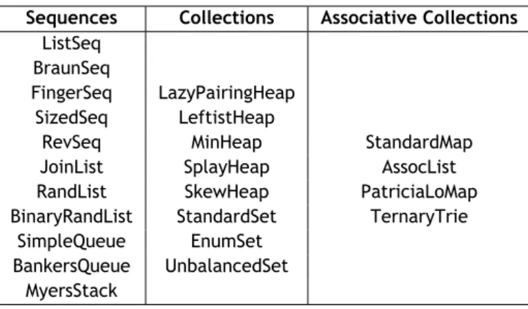
In Table 2.1 the different implementations available for the mentioned abstractions are pre-sented.

Table 2.1: Abstractions and Implementations available in Edison.

Sequences Collections Associative Collections ListSeq

BraunSeq

FingerSeq LazyPairingHeap SizedSeq LeftistHeap

RevSeq MinHeap StandardMap JoinList SplayHeap AssocList RandList SkewHeap PatriciaLoMap BinaryRandList StandardSet TernaryTrie

SimpleQueue EnumSet BankersQueue UnbalancedSet

MyersStack

In the remainder of this chapter, we describe in detail the different abstractions and implemen-tations provided by the library. In section 2.1 we describeSequences; in section 2.2 we present

Collections; finally, in section 2.3 we describeAssociative Collections.

2.1 The Sequence abstraction

TheSequenceabstraction models a conceptual data-structure type, in which different extremi-ties are distinguished and a specific insertion/removal order, is favored. InEdison, theSequence

abstraction includes, e.g., lists, queues and stacks. Furthermore, all implementations of this abstraction define a reusable, coherent and uniform set of functions.

Examples of functions (and their types) defined overSequencesare: lcons :: a→ Seq a → Seq a1 and rcons :: a→ Seq a → Seq a, which given an element of type a and a sequence of elements of type a, Seq a, produce a new sequence of the same type, obtained by inserting that element at the left, or right, of the original sequence, respectively; concat :: Seq (Seq a) → Seq a

1

InHaskell, the notation e :: t is used to declare that expression e is of type t. Also, the notation f :: a→ b is used to declare the type of a function f as “Taking (as input) something of type a to (and producing as output) something of type b”.

(30)

which given a sequence, Seq (Seq a), containing a number of sequences of elements of type a, gathers all the elements in those sequences in one sequence of elements of type a, Seq a; and map :: (a → b) → Seq a → Seq b which, given a function f, taking a value of type a and producing a value of type b, i.e., f :: a→ b, will apply f to all elements of a sequence of a typed elements, Seq a, transforming all elements to b typed elements, thereby producing as a result a sequence of elements of type b, Seq b.

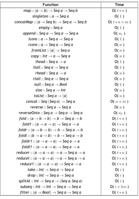
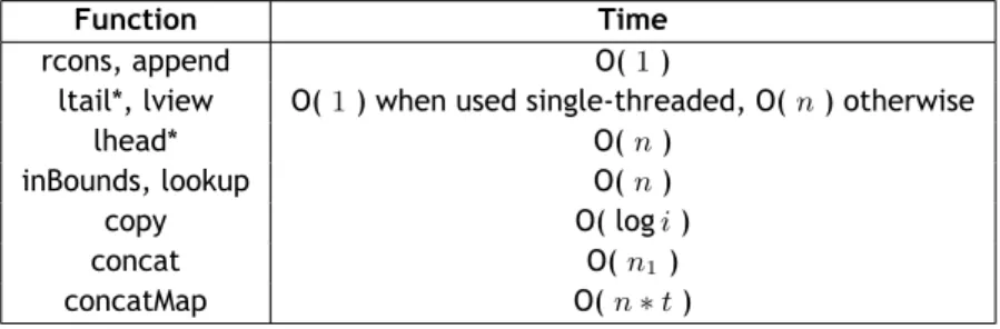
The functions defined by theSequenceabstraction have associated, theoretical, asymptotic run-ning time complexities, against which the corresponding complexities for all concrete imple-mentations, compare. These default running times are presented in Table 2.22.

Table 2.2: Default asymptotic time complexities for Sequences.

Function Time

map :: (a→ b) → Seq a → Seq b O( t∗ n )

singleton :: a→ Seq a O( 1 )

concatMap :: (a→ Seq b) → Seq a → Seq b O( t∗ n + m )

empty :: Seq a O( 1 )

append :: Seq a→ Seq a → Seq a O( n1)

lcons :: a→ Seq a → Seq a O( 1 )

rcons :: a→ Seq a → Seq a O( n )

fromList :: [a]→ Seq a O( n )

copy :: Int→ a → Seq a O( n )

lhead :: Seq a→ a O( 1 )

ltail :: Seq a→ Seq a O( 1 )

rhead :: Seq a→ a O( n )

rtail :: Seq a→ Seq a O( n )

null :: Seq a→ Bool O( 1 )

size :: Seq a→ Int O( n )

toList :: Seq a→ [a] O( n )

concat :: Seq (Seq a)→ Seq a O( n + m )

reverse :: Seq a→ Seq a O( n )

reverseOnto :: Seq a→ Seq a → Seq a O( n1) fold :: (a→ b → b) → b → Seq a → b O( t∗ n ) fold1 :: (a→ a → a) → Seq a → a O( t∗ n ) foldr :: (a→ b → b) → b → Seq a → b O( t∗ n ) foldl :: (b→ a → b) → b → Seq a → b O( t∗ n ) foldr1 :: (a→ a → a) → Seq a → a O( t∗ n ) foldl1 :: (a→ a → a) → Seq a → a O( t∗ n ) reducer :: (a→ a → a) → a → Seq a → a O( t∗ n ) reducel :: (a→ a → a) → a → Seq a → a O( t∗ n ) reduce1 :: (a→ a → a) → Seq a → a O( t∗ n )

take :: Int→ Seq a → Seq a O( i )

drop :: Int→ Seq a → Seq a O( i )

splitAt :: Int→ Seq a → (Seq a, Seq a) O( i ) subseq :: Int→ Int → Seq a → Seq a O( i + len ) filter :: (a→ Bool) → Seq a → Seq a O( t∗ n )

2

Function “families” like fold* and reduce* include strict versions which are not presented.

(31)

Table2.2 – continued from previous page

partition :: (a→ Bool) → Seq a → (Seq a, Seq a) O( t∗ n ) takeWhile :: (a→ Bool) → Seq a → Seq a O( t∗ n ) dropWhile :: (a→ Bool) → Seq a → Seq a O( t∗ n ) splitWhile :: (a→ Bool) → Seq a → (Seq a, Seq a) O( t∗ n )

inBounds :: Int→ Seq a → Bool O( i )

lookup :: Int→ Seq a → a O( i )

lookupWithDefault :: a→ Int → Seq a → a O( i ) update :: Int→ a → Seq a → Seq a O( i ) adjust :: (a→ a) → Int → Seq a → Seq a O( i + t ) mapWithIndex :: (Int→ a → b) → Seq a → Seq b O( t∗ n ) foldrWithIndex :: (Int→ a → b → b) → b → Seq a → b O( t∗ n ) foldlWithIndex :: (b→ Int → a → b) → b → Seq a → b O( t∗ n )

zip :: Seq a→ Seq b → Seq (a, b) O( min(n1, n2)) zipWith :: (a→ b → c) → Seq a → Seq b → Seq c O( t∗ min(n1, n2))

unzip :: Seq (a, b)→ (Seq a, Seq b) O( n ) unzipWith :: (a→ b) → (a → c) → Seq a → (Seq b, Seq c) O( t∗ n )

In Table 2.2, and in the implementation specific tables, presented later, the timings are given, generally, in terms of, n, the size of a single parameter sequence; t, the running time of a parameter function; n1and n2, the sizes of two parameter sequences; m, the size of an output sequence; i, an index of an element of a sequence; and len, a length of a portion of a sequence. In the remainder of this section we describe in more detail each of theSequenceimplementations available inEdison.

2.1.1 The ListSeq implementation

The underlying data type for the ListSeq implementation is the standard list type defined in the Prelude3_:

type Seq a = [a]

The asymptotic time complexities of this implementation are the baseline for the library (as published in the module Data.Edison.Seq). Only the functions toList and fromList differ. The differences are presented in Table 2.3.

Table 2.3: Asymptotic time complexities, for the ListSeq implementation, that differ from the baseline.

toList, fromList O( 1 )

2.1.2 The BraunSeq implementation

The BraunSeq implementation relies on a balanced binary tree [DD09] as an underlying data-structure. It is encoded as the followingHaskelldata type:

3

The Prelude isHaskell’s standard library of functions.

(32)

data Seq a = E| B a (Seq a) (Seq a)

A tree might be empty, or a tree with an element at every branch and empty leaves.

In this implementation an invariant is maintained: the left subtree is either exactly the same size as the right subtree, or at most one element larger.

The asymptotic time complexities differ from the defaults for the functions in Table 2.4.

Table 2.4: Asymptotic time complexities, for the BraunSeq implementation, that differ from the baseline.

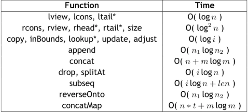
lview, lcons, ltail* O( log n ) rcons, rview, rhead*, rtail*, size O( log2n) copy, inBounds, lookup*, update, adjust O( log i )

append O( n1log n2)

concat O( n + m log m ) drop, splitAt O( i log n )

subseq O( i log n + len ) reverseOnto O( n1log n2)

concatMap O( n∗ t + m log m )

2.1.3 The FingerSeq implementation

The FingerSeq implementation realizes the Sequence abstraction, making use of a general-purpose data structure, a FingerTree [HP06]. The underlying data type is4_:

data Digit a =One a | Two a a | Three a a a | Four a a a a

data Node v a = Node2!va a| Node3 !va a a data FingerTree v a

=Empty | Single a

| Deep !v !(Digit a) (FingerTree v (Node v a)) !(Digit a) newtype Seq a = Seq (FingerTree SizeM (Elem a))

No asymptotic time complexities are given in the documentation for the FingerSeq implemen-tation. But, looking at the source code for FingerSeq we conclude that quite a number of the functions defined there, are implemented with a simple: unwrap from the Seq constructor, compute with FingerTree provided function and rewrap in the Seq constructor, style, for exam-ple, for rcons: rcons x = Seq◦ FT.rcons (Elem x) ◦ unSeq. Therefore, the few, time complexities given for FingerTree are “the same” for FingerSeq. From these, those that differ from the default complexities listed earlier, are presented in Table 2.5.

2.1.4 The SizedSeq implementation

The SizedSeq implementation is not really a sequence implementation. It is an adaptor over a parameter, existing, implementation. It keeps track of the sequence size explicitly.

4_{The !v is used to make the evaluation of v, strict/eager (Haskell}

’s default is lazy). 10

(33)

Table 2.5: Asymptotic time complexities, for the FingerSeq implementation, that differ from the baseline. Function Time rcons O( 1 ) rview O( 1 ) append O( log(min(n1, n2)))

The underlying data type is: data Sized s a = N !Int (s a) The N data constructor wraps:

• the s a; a sequence implementation s in which the elements are of type a; • an Int, which is the size of the sequence.

All operations time complexities are those of the underlying implementation, except that of the size operation, given in Table 2.6

Table 2.6: Asymptotic time complexities, for the SizedSeq implementation, that differ from the baseline.

Function Time size O( 1 )

2.1.5 The RevSeq implementation

The RevSeq implementation is also an adaptor for previously existing implementations.

It reverses the order of the elements in the wrapped sequence implementation. This adaptor is useful if an implementation has, for example, fast access times in its right-hand side, but we want to revert this to the left-hand side. This adaptor also keeps track of the sequence size. The underlying data type is:

data Rev s a = N !Int (s a)

This datatype is the same datatype as for the SizedSeq adaptor.

The asymptotic time complexities for the application of this adaptor over a underlying existing implementation are determined by that implementation, except that the access times for both sides of the sequence are exchanged. Also the size operation time complexity differs as stated in Table 2.7.

Table 2.7: Asymptotic time complexities, for the RevSeq implementation, that differ from the baseline.

Function Time size O( 1 )

2.1.6 The JoinList implementation

The JoinList sequence implementation is based on a tree data-structure [KoC15], which might be empty (E), or will contain elements only in it’s leaves (L a)5_.

5

This tree data-structure is called a leaftree.

(34)

The underlying data type is:

data Seq a = E| L a | A (Seq a) (Seq a)

An invariant: E never a child of A, must be maintained.

Table 2.8: Asymptotic time complexities, for the JoinList implementation, that differ from the baseline.

rcons, append O( 1 )

ltail*, lview O( 1 ) when used single-threaded, O( n ) otherwise

lhead* O( n )

inBounds, lookup O( n )

copy O( log i )

concat O( n1 )

concatMap O( n∗ t )

2.1.7 The RandList implementation

The RandList implementation aims to provide a data-structure that supports both efficient ac-cess to random elements contained in it, and primitive list operations (head, cons, tail) that run as fast as their native list counterparts [Oka95a].

That data-structure is a list of complete binary trees [She09] with elements of a type a. The underlying data type is:

data Tree a = L a| T a (Tree a) (Tree a) data Seq a = E| C !Int (Tree a) (Seq a) Two invariants must be maintained:

• the list of complete binary trees is maintained in non-decreasing order of size;

• the first argument to the data-construtor C is the number of nodes in the encapsulated tree.

The asymptotic time complexities differ from the defaults for the funtcions in Table 2.9.

Table 2.9: Asymptotic time complexities, for the RandList implementation, that differ from the baseline.

Function Time rhead*, size O( log n ) copy, inBounds O( log i ) lookup*, update, adjust, drop O( min(i, log n) )

subseq O( min(i, log n) + len )

2.1.8 The BinaryRandList implementation

The BinaryRandList implementation represents a linear data structure, which may be empty (with the E data constructor) or have two distinct recursive cases that model the fact that the list has an even (with the Even data constructor), or odd (with the Odd data constructor), number of elements [Oka99].

The underlying data type is: 12

(35)

data Seq a = E| Even (Seq (a, a)) | Odd a (Seq (a, a))

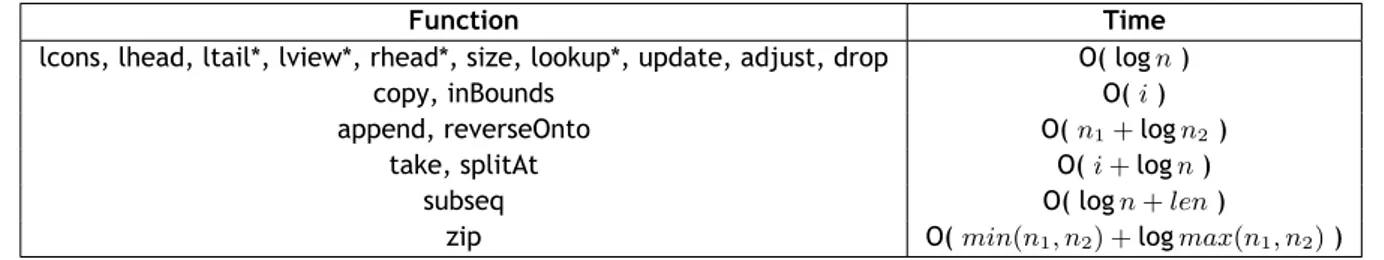
Table 2.10: Asymptotic time complexities, for the BinaryRandList implementation, that differ from the baseline.

lcons, lhead, ltail*, lview*, rhead*, size, lookup*, update, adjust, drop O( log n )

copy, inBounds O( i )

append, reverseOnto O( n1+log n2)

take, splitAt O( i + log n )

subseq O( log n + len )

zip O( min(n1, n2) +log max(n1, n2))

2.1.9 The SimpleQueue implementation

The SimpleQueue implementation of the Sequence abtraction is based on two lists. One repre-senting the front of the queue, and the second, the rear of the queue.

The underlying data type is: data Seq a = Q [a] [a]

That is the data constructor Q encapsulates the two standardHaskelllists mentioned before. The rear is maintained in reverse order, the first element of the rear list is actually the last element of the sequence.

An invariant must be obeyed/maintained: the front will be empty only if the rear is also empty. This guarantees that the first element of the queue can always be accessed in O( 1 ) time [Oka99]. The asymptotic time complexities differ from the defaults for the functions in Table 2.11.

Table 2.11: Asymptotic time complexities, for the SimpleQueue implementation, that differ from the baseline.

rcons, fromList O( 1 )

lview, ltail* O( 1 ) if single threaded, O( n ) otherwise inBounds, lookup, update, drop, splitAt O( n )

2.1.10 The BankersQueue implementation

The BankersQueue implementation of the Sequence abtraction is similar to the SimpleQueue implementation. The differences are that the size of the sequence is tracked explicitly and a different invariant is abided by.

data Seq a = Q !Int [a] [a] !Int

That is, the Q data constructor encapsulates two Ints and two lists. The first list represents the front of the queue; the second list represents the rear of the queue. The first Int is the length (or size) of the front, and the second the length of the rear. The rear list is maintained in reverse order (the first element is the last element of the sequence).

An invariant must be obeyed/maintained: the front will be at least as long as the rear [Oka95b]. The asymptotic time complexities differ from the defaults for the functions in Table 2.12.

(36)

Table 2.12: Asymptotic time complexities, for the BankersQueue implementation, that differ from the baseline.

Function Time rcons, size, inBounds O( 1 )

2.1.11 The MyersStack implementation

The MyersStack sequence implementation is a realization of the stack abstraction which also permits accesses to the kth element [Mye83].

data Seq a = E| C !Int a (Seq a) (Seq a)

This represents a binary tree (as already stated for other implementations).

Table 2.13: Asymptotic time complexities, for the MyersStack implementation, that differ from the baseline.

Function Time lookup, inBounds, drop O( min(i, log n) )

rhead*, size O( log n ) subseq O( min(i, log n) + len )

2.2 The Collection abstraction

The Collectionsabstraction includes Setsand Heaps(priority queues where the priority is the element). In this thesis Heaps and Sets are described in detail in sections 2.2.1 and 2.2.2 re-spectively.

ACollectioninEdisonis characterized by whether or not it satisfies three properties:

1. observability: whether the elements in a collections can, or not, be recovered from the collection.

2. ordering: whether the type of elements in a collection satisfies a total ordering require-ment;

3. uniqueness: whether the elements in a collection are distinct;

Currently allCollectionsinEdisonabide by the observability and ordering properties, withSets

also guarantying the uniqueness of the elements stored in them.

No default asymptotic time complexities are provided for this abstraction. Regarding specific implementations there is only one source of such complexities, the Data.Set library, which is the underlying implementation for the StandardSet realization of the abstraction.

2.2.1 Heaps

AHeapis aCollection, generally based on a tree shaped data structure, and usually maintaining the minimum (it could also be the maximum) element readily available for “inspection”. That is, determining the minimum element should be an computationally inexpensive operation. 14

(37)

2.2.1.1 The LazyPairingHeap implementation

The LazyPairingHeap implementation is a heap-ordered tree which can branch one-way, or two-way, depending on the number of (odd or even) children[Oka99].

data Heap a = E| H1a (Heap a)| H2a !(Heap a) (Heap a)

A well-formed LazyPairingHeap abides by the invariant: the left child of a H2node must not be empty.

2.2.1.2 The LeftistHeap implementation

A LeftistHeap is a heap implementation based on a heap ordered binary tree [Oka99]. Being heap ordered means that whatever the node in the tree, the element contained in it is no larger than the elements in the nodes of it’s subtrees. Also the tree must conform to the so-called leftist property. This property states that for any node, the rank of it’s left subtree is no lesser than the rank of it’s right subtree. The rank of a node is defined to be, the length of the rightmost path from that node to an empty node (the length of the node’s right spine).

data Heap a = E| L !Int !a !(Heap a) !(Heap a)

2.2.1.3 The MinHeap implementation

The MinHeap “implementation” is really just an adaptor for other heap implementations, that keeps the minimum element separately.

The underlying data type is: data Min h a = E| M a h

2.2.1.4 The SplayHeap implementation

The SplayHeap collection implementation is based on a splay tree [ST85]. A splay tree is similar to a balanced binary search tree. In a splay tree the balancing is carried out as operations over the data struture are performed, by way of transformations that tend to increased the balance, but no explicit information regarding that purpose is kept inside the data structure [Oka99]. Data structures behaving in this way are usually calledself-adjusting.

data Heap a = E| T (Heap a) a (Heap a)

The elements in the heap are maintained in binary search tree order [SW14a] (duplicates al-lowed).

2.2.1.5 The SkewHeap implementation

The SkewHeap data structure is a self-adjusting implementation akin to the LeftistHeap imple-mentation [ST86].

data Heap a = E| T a (Heap a) (Heap a)

(38)

2.2.2 Sets

ASetis aCollectionin wich no duplicate elements are allowed.

Characteristic functions defined over Sets are, for example: intersection :: Set a → Set a → Set a, which computes the common elements of two sets, and difference :: Set a → Set a → Set a, which calculates the member elements of a set not members of another set, both taking two sets of elements of type Set a and producing another set of the same type, and subset :: Set a→ Set a → Bool which returns a True or False (Bool6_{) value indicating if the first parameter} set is a subset of the second parameter set.

2.2.2.1 The StandardSet implementation

The StandardSet implementation is just a wrapper around the standardHaskelllibrary Data.Set. The Data.Set implementation is based on size balanced binary trees [NR72].

The underlying data type is: type Set = Data.Set.Set

2.2.2.2 The EnumSet implementation

In this implementation of theSetabstraction, its instances (sets) are realized recurring to “bit strings” and bitwise operations over those “strings”.

The underlying data type is: newtype Set a = Set Word

This set implementation can only be used to model sets for which the maximum number of elements that may appear in the set is less than or equal to the number of bits in the Word7 type.

2.2.2.3 The UnbalancedSet implementation

In this implementation a set is modeled as an unbalanced binary search tree. In such a tree no equilibrium in the distribution of nodes/elements is enforced, and as such, the performance of operations over the tree may degenerate into that of a simple list.

data Set a = E| T (Set a) a (Set a)

On instances of this datatype an invariant is maintained, the binary search tree order [SW14a]. That is, for any node with an element y, all elements in the left subtree are lesser than y, and, all elements in the right subtree are greater than y.

2.3 Associative Collections

TheAssociative Collectionsabstraction includes e.g., finite maps, finite relations and priority queues (with distinct priority and element8_{). They generically map keys of a type k to values of}

6

TheHaskellBoolean type.

7_The_Haskell_{Word type is an unsigned integral type, of size equal to that of the type Int.} 8

Whereas in a queue the priority is drawn from the insertion order, here the priority is a stand-alone value.

(39)

a type a. Exceptions are the PatriciaLoMap and TernaryTrie implementations which use more restricted types of keys (Int and [k] respectively). The other implementations respect the same

API.

Associative Collections, like Collections, are charaterized by the three proterties already mentioned for the later, observability, ordering and uniqueness.

No default asymptotic time complexities are provided for this abstraction. Regarding specific implementations there is only one source of such complexities, the Data.Map library, which is the underlying implementation for the StandardMap realization of the abstraction.

In the remainder of this section we describe the available implementations inEdison.

2.3.1 The StandardMap implementation

The StandardMap implementation is just a wrapper around the standardHaskelllibrary Data.Map. The Data.Map implementation is based on size balanced binary trees [NR72].

The underlying data type is therefore: type FM = Data.Map.Map

2.3.2 The AssocList implementation

The AssocList implementation realizes theAssociative Collectionsabstraction via an associa-tion list [Wik16]. An associaassocia-tion list is basically a collecassocia-tion of pairs in which one of the compo-nents is called the key, and the other is called the value. Each such pair is interpreted as one mapping from the key to the value, in the list.

data FM k a = E| I k a (FM k a)

In the AssocList implementation duplicate associations are removed conceptually, but not physi-cally. If duplicate associations are found then the first occurrence of a key is the one considered to be in the map.

2.3.3 The PatriciaLoMap implementation

The PatriciaLoMap implementation realizes finite maps based on little-endian patricia trees [OG98]. The underlying data type is:

data FM a = E| L Int a | B Int Int !(F M a) !(F M a)

The PatriciaLoMap implementation abides by a number of invariants, e.g. “no B node has an E child”.

2.3.4 The TernaryTrie implementation

The TernaryTrie implementation models finite maps as ternary search tries9_[SW14b].

A ternary search trie is a tree shaped structure, in which, each node branches into three sub-trees. Also each node contains a part of a key which will ultimately lead to a value associated

9

Trie is pronounced as try!

(40)

with the whole of that key. The three subtrees are associated with a part of a key that is consid-ered to be lesser, equal or greater than the part stored at the node from which those subtrees stem from.

The tree structure is kept balanced. The underlying data type is:

data FM k a = FM !(M aybe a) !(F M B k a)

data FMB k v = E| I !Int !k !(Maybe v) !(F MB k v) !(F MB′ k v) !(F M B k v) newtype FMB′k v = FMB′(FMB k v)

2.4 Final Remarks

In this chapter, we have described a software library that offers a number of purely functional implementations, for three different data structure abstractions. This library will be our ob-ject of study. In the next chapter we will present the “environment” in which our study was conducted, and the tools used to perform this study.

(41)

Chapter 3

Experimental Setting

In Chapter 2, we have described a library of several different implementations for common data structure abstractions, Edison.

In order to evaluate the performance of those data structure implementations according to some criteria, we need to create programs (“functions”) that make use of those implementations, and execute these functions (run the programs) while measuring certain characteristics of interest. The set of functions/programs to run is called a benchmark. The benchmark (operations/components) used in this work is described in Section 3.1.

To actually execute the “programs” of the benchmark and record the measures of interest, we make use of a benchmarking tool named Criterion, described in Section 3.2.

In Section 3.3, we allude to the underlying technology that allows us to gather the energy consumption measures, that are the driving purpose of this study, the RAPL interface[Cou14]. Finally, in Section 3.4, the underlying hardware/software setup used in the execution of our measuring is presented.

3.1 The Benchmark

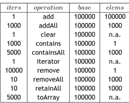
Following the approach considered in different studies [PCS+_{16, MPC14, Ca14, PLCL16], our} benchmark is inspired by the microbenchmark to evaluate the run time performance of Java’s JDK (Java Development Kit) Collection API (Application Programming Interface) implementa-tions, presented in [Lew11]. The operations that are defined in such benchmark are listed in Table 3.1.

Table 3.1: Benchmark Operations.

iters operation base elems

1 add 100000 100000 1000 addAll 100000 1000 1 clear 100000 n.a. 1000 contains 100000 1 5000 containsAll 100000 1000 1 iterator 100000 n.a. 10000 remove 100000 1 10 removeAll 100000 1000 10 retainAll 100000 1000 5000 toArray 100000 n.a.

All the operations can be abstracted by the format:

iters∗ operation(base, elems)

This format reads as: iterate operation a given number of times (iters) over a data structure with a base number of elements. If operation requires an additional data structure, the number of elements in it is given by elems. All the operations are suggested to be executed over a base 19

(42)

structure with 100000 elements. So, the second entry in the table suggests adding 1000 times all the elements of a structure with 1000 elements to the base structure (of size 100000).

3.2 A library for implementing/conducting microbenchmarks

Criterion[O’S09] is a microbenchmarking library that is used to measure the performance of

Haskellcode. It provides a framework for both the execution of the benchmarks as well as the analysis of their results, being able to measure events with duration in the order of picoseconds.

Criterionis robust enough to filter out noise coming, e.g., from the clock resolution, the op-erating system’s scheduling or garbage collection. Criterion’s strategy to mitigate noise is to measure many runs of a benchmark in sequence and then use a linear regression model to esti-mate the time needed for a single run. That way, the outliers become visible.

Having been proposed in the context of a functional language with lazy evaluation, Criterion

natively offers mechanisms to evaluate the results of a benchmark in different depths, such as Weak Head Normal Form or Normal Form.

Criterionis able to measure CPU time, CPU cycles, memory allocation and garbage collection. In our work, we have utilized a modified version which has had its domain extended so that it is also able to measure the amount of energy consumed during the execution of a benchmark[Lim16]. The adaptation ofCriterionhas been conducted based on two essential considerations. First, the energy consumed in the sampling time intervals used byCriterionis obtained via external C function invocations to RAPL (Section 3.3). This is similar to the time measurements na-tively provided byCriterion, which are also realized via Foreign Function Interface1_{(FFI) calls.} Second, we need to handle possible overflows occurring on RAPL registers [DGH+_{10]. For two} consecutive reads x and y of values in such registers, this was achieved by discarding the en-ergy consumed in the corresponding (extremely small) time interval ify, which is read later, is smaller thanx.

In the extended version ofCriterion, energy consumption is measured in the same execution of the benchmarks which is used to measure runtime performance. In this version, all the afore-mentioned aspects of Criterion’s original methodology have straightforwardly been adapted for energy consumption analysis. The source code for the modified Criterion is available on GitHub2.

In the remainder of this section we will exemplify the usage of the library. Consider the source code in Listing 3.1.

This code defines the straightforward recursive version of the factorial function, taking one argument n, which calculates the factorial of a non-negative Integer number. It also defines the main3 _{function which makes use of the benchmarking machinery provided by Criterion. In} this main function we define:

• a group of benchmarks, with the bgroup function, named “factorialBGroup” (multiple groups of benchmarks are allowed);

• within this group, four benchmarks, each with it’s own label (“a” to “d”), with the bench function.

1_{The Foreign Function Interface is}_Haskell_{’s interfacing mechanism to software components}

writ-ten in other programming languages.

2_{https://github.com/green-haskell/criterion} 3

The main function in a Main module is the entry point to aHaskellprogram. 20

(43)

Listing 3.1 Criterion benchmark implementation example. import Criterion.Main

-- The function to benchmark.

factorial :: Integer -> Maybe Integer

factorial n

| n < 0 = Nothing

| otherwise = Just ( fact n ) where

fact :: Integer -> Integer fact 0 = 1

fact n = n * fact ( n - 1 )

-- Our benchmark harness.

main = defaultMain [

bgroup "factorialBGroup" [

bench "a" $ whnf factorial ( -1 ) , bench "b" $ whnf factorial 0 , bench "c" $ whnf factorial 2 , bench "d" $ whnf factorial 16 ]

]

We also use the whnf function to instruct Criterion, to evaluate the factorial function’s result to Weak Head Normal Form. It is also possible to request from Criterion the evaluation to Normal Form, using the nf function instead.

Function whnf receives as arguments the function to evaluate, saturated with all but the last of it’s parameters, and the evaluated function’s last parameter. These are the factorial function and each of the “-1”, “0”, “2”, “16” numbers, respectively.

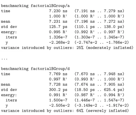
An example usage/output of such a benchmark is demonstrated in Figure 3.1. Executing the benchmark with the “--regress energy:iters” option (the first line in Figure 3.1) we get the (abbreviated) outputs following in that figure. The output is “broken” by benchmarks groups and benchmarks. In this example we have only one group of benchmarks, factorialBGroup, and four benchmarks, “a” to “d”, of which only two, “a” and “d” are pictured.

The output lines we are most interested in are thetime line, and the iters line.

The time line displays the estimated time taken by a single execution of the function being benchmarked. In the example output, benchmark “a” i.e., each execution of (factorial (−1)), runs in approximately 7.230 nanoseconds (ns). This estimation is obtained by a “Ordinary Least-Squares” (OLS) linear regression, obtained from the raw measurements (times to run a number of iterations/executions).

Theiters line, results from the same kind of procedure as the time line (OLS linear regression on raw measurements) but presents us with an estimate of the energy consumed by one execution of the function being benchmarked. For example, running benchmark “d”, tells us that an execution of the factorial 16 consumes around 1.5e-7 Joules (J).

The first value in each line is the main estimate for the measure in that line, the values in parentheses are lower and upper bounds on the estimate.

The R² lines (the first unlabeled line and energy labeled line) show a value that “measures” the accuracy of the linear regression. It’s called R² goodness-of-fit, and it’s value should lie between 0.99 and 1.

(44)

Figure 3.1: Modified Criterion, usage/output example.

test-fact --regress energy:iters benchmarking factorialBGroup/a time 7.230 ns (7.191 ns .. 7.279 ns) 1.000 R² (1.000 R² .. 1.000 R²) mean 7.231 ns (7.196 ns .. 7.272 ns) std dev 125.7 ps (110.1 ps .. 138.0 ps) energy: 0.995 R² (0.992 R² .. 0.997 R²) iters 1.326e-7 (1.303e-7 .. 1.345e-7) y -2.268e-2 (-2.747e-2 .. -1.766e-2) variance introduced by outliers: 25% (moderately inflated) ... benchmarking factorialBGroup/d time 7.769 ns (7.670 ns .. 7.948 ns) 0.997 R² (0.993 R² .. 1.000 R²) mean 7.728 ns (7.674 ns .. 7.905 ns) std dev 300.2 ps (18.50 ps .. 625.4 ps) energy: 0.991 R² (0.987 R² .. 0.994 R²) iters 1.500e-7 (1.446e-7 .. 1.547e-7) y -2.505e-2 (-3.149e-2 .. -1.917e-2) variance introduced by outliers: 64% (severely inflated)

A more detailed example/explanation, without the energy measuring extension, can be found on the tool author’s webpage athttp://www.serpentine.com/criterion/tutorial.html.

3.3 An interface for measuring energy consumption

Running Average Power Limit (RAPL) [DGH+_{10] is an interface provided by modern Intel} proces-sors, using the Sandy Bridge and successor microarchitectures (roughly, Core second generation microprocessors and successors), to allow setting custom power limits to the processor pack-ages. Using this interface one can access energy and power readings via a model-specific register (MSR). RAPL uses a software power model to estimate the energy consumption based on various hardware performance counters, temperature, leakage models and I/O models [WJK+_{12]. Its} precision and reliability has been extensively studied [RNA+_{12, HDVH12].}

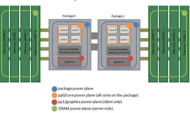
RAPL interfaces operate at the granularity of a processor socket (package). There are MSRs to access 4 domains:

• Package (PKG): total energy consumed by an entire socket • Power Plane 0 (PP0): energy consumed by all cores and caches

• Power Plane 1 (PP1): energy consumed by the on-chip Graphics Processing Unit (GPU) • Dynamic Random Access Memory (DRAM): energy consumed by all Dual In-line Memory

Modules (DIMMs)

The client (consumer desktop) platforms have access to {PKG, PP0, PP1} while the server plat-forms have access to {PKG, PP0, DRAM}. These domains are illustrated in Figure 3.24_.

4

Source:https://software.intel.com/en-us/articles/intel-power-governor

(45)

Figure 3.2: RAPL domains.

For this work, we collected the energy consumption data from the PKG domain using themsr module of the Linux kernel to access the MSR readings.

3.4 The test-bed

For this study, all experiments were conducted on a machine with 2x10-core Intel Xeon E5-2660 v2 processors (Ivy Bridge microarchitecture) and 256GB of DDR3 1600MHz memory. This machine runs the Ubuntu Server 14.04.3 LTS (Linux kernel 3.19.0-25) Operating System (OS). The compiler was Glasgow Haskell Compiler (GHC) 7.10.2, using Edison 1.3 (Chapter 2), and the modified Criterion (Section 3.2) library. Also, all experiments were performed with no other load on the OS.

3.5 Final Remarks

In this chapter, we have described the benchmark on which our work is based, the benchmarking tool, Criterion, used to measure both execution time and energy consumption of the benchmark and the RAPL interface which allows us gather the energy consumption measures from the pro-cessor MSRs.

Together with the Edison library, described in Chapter 2, this comprises all the technology needed to perform our proposed study.

In the next chapter, we shall describe the methodology followed, while undertaking that study.

(46)

Energy Consumption of Functional Programs in the Context of Lazy Evaluation

UNIVERSIDADE DA BEIRA INTERIOR

Engenharia