Felipa De Mello-Sampayo
To cite this version:
Felipa De Mello-Sampayo. Competing-Destinations Gravity Model: An Application to the Geographic Distribution of FDI. Applied Economics, Taylor & Francis (Routledge), 2009, 41 (17), pp.2237-2253. .
HAL Id: hal-00582176
https://hal.archives-ouvertes.fr/hal-00582176
Submitted on 1 Apr 2011HAL is a multi-disciplinary open access archive for the deposit and dissemination of sci-entific research documents, whether they are pub-lished or not. The documents may come from teaching and research institutions in France or abroad, or from public or private research centers.
L’archive ouverte pluridisciplinaire HAL, est destin´ee au d´epˆot et `a la diffusion de documents scientifiques de niveau recherche, publi´es ou non, ´emanant des ´etablissements d’enseignement et de recherche fran¸cais ou ´etrangers, des laboratoires publics ou priv´es.
For Peer Review
Competing-Destinations Gravity Model: An Application to the Geographic Distribution of FDI
Journal: Applied Economics Manuscript ID: APE-06-0557 Journal Selection: Applied Economics
JEL Code:
F21 - International Investment|Long-Term Capital Movements < F2 - International Factor Movements and International Business < F - International Economics, F23 - Multinational Firms|International Business < F2 - International Factor Movements and International Business < F - International Economics, C23 - Models with Panel Data < C2 - Econometric Methods: Single Equation Models < C - Mathematical and Quantitative Methods
For Peer Review
Competing–Destinations Gravity Model: An Application to the
Geographic Distribution of FDI
Felipa de Mello-Sampayo† †
ISCTE-Higher Institute for Labour and Business Studies, Economics Department
Abstract
The competing–destinations formulation of the gravity model ensues from the fact that unlike the classical version, this approach explicitly acknowledges the interdependence of the flows between a set of alternative locations, i.e. countries-recipients are competing for FDI. This paper examines empirically a range of theoretical hypotheses about the determinants of FDI location in a panel data regression framework. The results of the estimation of a gravity model lend support to the proximity-concentration and internalization hypotheses. Also, the fact that FDI has been found to be decreasing in the competition posed by alternative locations is suggestive of the superiority of the competing–destinations version of the gravity equation over its classical formulation.
JEL Classification: C23; F21; F23
Keywords: Gravity Model, Foreign Direct Investment, Multinational Enterprizes
Postal address: ISCTE, Department of Economics, Av. For¸cas Armadas, 1649–026, Lisbon,
Portugal.
Author’s email: [email protected]
3 4 5 6 7 8 9 10 11 12 13 14 15 16 17 18 19 20 21 22 23 24 25 26 27 28 29 30 31 32 33 34 35 36 37 38 39 40 41 42 43 44 45 46 47 48 49 50 51 52 53 54 55 56 57 58 59 60
For Peer Review
1
Introduction
The gravity equation has been widely used to understand spatial interaction patterns, mainly the international trade and Foreign Direct Investment (FDI) flows between different geographical entities. However, under the gravity equation, a Multinational Enterprize (MNE) is supposed to choose a country to invest in from an one-shot decision-making process, since it implies that FDI flows between two countries depend solely on factors pertaining to those countries. However, the decision of location of FDI is usually considered to be a result of a two-stage decision-making process. The first stage consisting of choosing a possible set of countries to invest in and the second stage consisting of the firm choosing a specific country from that set of countries, e.g. a vertical FDI decision by an MNE involves picking the “best” low–cost host at the expense of other potential host locations (Blonigen, 2005). Hence, as contended by Fotheringham (1983a,b, 1984), if this two–stage decision–making process prevails, the classical gravity models are mis–specified. The superiority of the competing–destinations formulation of the gravity model ensues from the fact that unlike the classical version, this approach explicitly acknowledges the interdependence of the flows between a set of alternative locations (Fotheringham, 1983a, Hua and Porell, 1979, Roy, 2004, Thorsen and Gitlesen, 1998).
The particular version of the competing–destinations gravity model that we employ is the share gravity model proposed in de Mello-Sampayo (2006) and summarily described in §2. In short, the share version of the gravity model adds to the classical version a competition factor that captures the gravity of “rival” countries candidate to the U.S. FDI. The competition factor allows to treat the U.S. FDI directed to one specific location as interdependent with the FDI decisions concerning alternative locations. In the sense that the validity of the share version of the gravity model implies that the classical version (that has been extensively used in empirical applications in international economics) is misspecified, testing the empirical validity of the share version constitutes a central goal of this paper.
As globalization reaches the remotest economies in the world, an increasing number of firms engage in FDI for an increasing number of reasons, in a widening array of locations, in order to take advantage of the spawning business opportunities and also to better accommodate the blis-tering pace of technological change. MNEs have undergone considerable organizational changes and important contributions have been made to model different forms and degrees of involve-ment of business firms in foreign activities (Carr, Markusen and Markus, 2001, Ekholm, Forslid and Markusen, 2006, Helpman, 2006, Markusen, 2002). However, the traditional trade theory continues to explain a considerable part of the trade and FDI flows (see Helpman, 2006). From the traditional trade theory, we test the “proximity-concentration” hypothesis, the “factor pro-portions” and the “internalization” hypothesis, acknowledging the fact that countries-recipients are competing for FDI.
The mode of foreign penetration (e.g. FDI versus exporting) is not under scrutiny, nor are the factors that lead a firm to engage in FDI nor is spatial and organizational configuration of MNE´s activities. What is relevant in this paper is what leads a MNE to choose one location to the detriment of others.
Previous work has shown that FDI flows respond to a wide myriad of variables, which implies that an empirical application based on a specific theoretical framework will necessarily provide a partial account of the locational determinants of FDI that may, inclusively, lead to erroneous conclusions (omitted variable bias). The gravity equation constitutes a very useful empirical framework for the study of FDI location, since it allows combining several explanatory variables without being hostage to any particular theoretical framework.
This paper pursues an eclectic approach that accommodates several variables in order to provide an overall view of the determinants that lead MNEs to choose a particular foreign
pro-3 4 5 6 7 8 9 10 11 12 13 14 15 16 17 18 19 20 21 22 23 24 25 26 27 28 29 30 31 32 33 34 35 36 37 38 39 40 41 42 43 44 45 46 47 48 49 50 51 52 53 54 55 56 57 58 59 60
For Peer Review
duction location over others and at the same time test the most prominent traditional theories of FDI location. Looking at the related literature, our paper comes closest to Brainard (1997). As in there, we use data on U.S. MNEs to test the proximity-concentration, factor-proportions and internalization hypotheses and arrive at similar qualitative conclusions. However, unlike Brainard (1997) who takes a cross-section approach, we carry out our estimation within a panel data framework, which arguably allows us to get more reliable estimates and inference. More-over, unlike Brainard (1997) who uses the classical version of the gravity model, we use the share gravity formulation, which includes a competition factor that according to de Mello-Sampayo (2006) enhances the specification of the gravity model for the analysis of the location of multi-national activity.
The structure of the paper is as follows. First, the share gravity model is introduced and the related literature reviewed. The data and the estimation method are described and the results of the share gravity model analyzed and discussed.
2
The Share Gravity Model
The formulation adopted in most applications of the gravity models to the analysis of trade and FDI goes back to the contribution of Hua and Porell (1979) and can be summarized by the generalized version of the classical gravity model, as follows:
Fijt= Ω · AGα1
it · ATjtα2· SFijtα3 (1)
where Fijt is the expected interaction flow between locations i and j per unit of time, Ω is a
predetermined quantity, AGit measures the features of country i that generate the outflows,
ATjt measures the attractiveness of country j and SFijt is a spatial measure between the two
countries. Hua and Porell (1979) denominate AGit, ATjt, SFijt, as generation, attraction (the
mass terms) and the spatial term, respectively. So, the inverse of the facility, SFijt−1, measures the separation factor, which in the present context certainly includes transport costs between country i and j, at time t, but also any trade and foreign investment barriers in the target destination, j. α1, α2 and α3 are parameters to be estimated.
The classical gravity model applied to the international trade theory uses the “distance-decay” concept (Fotheringham, 1983a, 1984), which may be described as the rate at which the volume of trade between locations decreases as the distance between them increases. Conversely, the FDI theory uses the “distance-incentive” concept, or the rate at which the volume of FDI flow increases as the transport costs between economic centers increases, since it will become preferable to produce locally than to export (Horstmann and Markusen, 1992, Brainard, 1993b, 1997, Markusen and Venables, 1996). Therefore, when modeling international trade flows we expect that α1 > 0, α2 > 0 and α3 < 0 whereas for FDI flows we should obtain α1 > 0, α2 > 0
and α3> 0.
In spite of its widespread use in international economics, the classical version of the gravity model arguably contains a fundamental flaw when applied to the empirical analysis of FDI: it implies that FDI flows between two countries depend solely on factors pertaining to those countries. Most crucially it ignores the attractiveness of alternative locations. To overcome this limitation de Mello-Sampayo (2006) proposes the use of the share version of the gravity model introduced in the human geography literature by Hua and Porell (1979), but virtually ignored in economic applications. Its main difference from the classical version stems from the fact that a competition factor encompassing the ability of third countries to attract FDI is included as a dampening factor to FDI flowing to any potential location. Such an alternative specification of
3 4 5 6 7 8 9 10 11 12 13 14 15 16 17 18 19 20 21 22 23 24 25 26 27 28 29 30 31 32 33 34 35 36 37 38 39 40 41 42 43 44 45 46 47 48 49 50 51 52 53 54 55 56 57 58 59 60
For Peer Review
the gravity model applied to the behavior of FDI may be given by the following equation:
Fijt= Ω · (AGjt)β0· (ATit)β1·(SF1 ijt)β2 · 1 (CFijt)β3 (2) CFijt= N X k6=i ATkt· 1 SFijt (3) where β0, β1, β2 and β3 are parameters, i stands for country, j for industry, t for time, US for
United States. The variable FU S
ijt denotes United States FDI into industry j of country i at time
t.
Equation (3) gives the sum, weighted by the separation term relative to industry j, of all other countries’ characteristics (except country i) in attracting FDI from the United States. Equation (3) attempts to capture the gravity of the competing destinations. Otherwise, it can be seen as a composite index that yields the competition faced by industry j in country i in attracting United States FDI.
Since the aim of the present study is not to explain the amount in levels of FDI, but rather the way United States MNEs distribute their foreign activities across different countries, we need a model of shares rather than levels. That may be accomplished by substituting the parameter Ω in equation (2) by the total FDI outflow from United States in industry j into all countries in the panel, F∗jt, to yield the share distribution gravity model:
Fijt F∗jt = (ATit) β1 · 1 (SFijt)β2 · 1 (CFijt)β3 (4)
Notice that we have not included the generation variable in equation (4) since this is an origin-specific model and so variations in the United States’ aggressiveness become redundant in explaining changes in the FDI shares of destination countries1. What is crucial about equation
(4) is the fact that since a country’s advantage as a location for FDI is dependent on the weighted sum of all other countries’ attractiveness, the traditional gravity model, according to which a change in the characteristics of one country would not shift flows into other countries, misses the interdependence among FDI flows. However, in a world of scarce capital resources, the interdependence of the flows seems to be a much more plausible theory of investment.
3
Related Literature
The proximity-concentration hypothesis explains the firm’s choice between the two alternatives modes of foreign penetration, exporting and overseas expansion, as depending on the trade-off between the advantages related to proximity to the foreign market and the economies of scale that might result from the concentration of production (Krugman, 1983, Horstmann and Markusen, 1992, Brainard, 1993b, 1997). The models that underlie this hypothesis assume that each firm operate within a differentiated goods sectors. This sector is characterized by increasing returns at the firm level due to some input that can be easily spread among different production facilities, scale economies at the plant level, such that unit costs are decreasing with the plant size, and a variable transport cost. In this setup, and ignoring factor-proportions discrepancies, the proximity-concentration hypothesis predicts that FDI will tend to prevail relative to exporting the more difficult is the access to the foreign market, i.e. the higher are transport costs and 1If the level of flows instead of shares was to be analyzed, the home country’s aggressiveness would prove
instrumental in accounting for variations in the interaction flows. 3 4 5 6 7 8 9 10 11 12 13 14 15 16 17 18 19 20 21 22 23 24 25 26 27 28 29 30 31 32 33 34 35 36 37 38 39 40 41 42 43 44 45 46 47 48 49 50 51 52 53 54 55 56 57 58 59 60
For Peer Review
trade barriers, and the lower are the economies of scale at the plant level relative to those at the firm level. Since the market-size hypothesis holds that if there are economies of scale firms will tend to invest in the larger foreign markets and export to the smaller ones in order to reap scale advantages and minimize transport costs, it can be said that the proximity-concentration hypothesis nests the market-size hypothesis of FDI location.
The factor-proportions hypothesis (Helpman, 1984, Markusen, 1984, Helpman and Krugman, 1985, Ethier and Horn, 1990) explains FDI location in terms of the combination of relative factor endowments with the characteristics of the production technology. In this context, if the production technology is such that different production stages have different factor-intensities, FDI may emerge as a viable way of exploiting lower factor costs. In the simplest case, where headquarters activities are capital-intensive and plant activities are labor-intensive, a single-plant MNE might emerge in order to exploit different factor costs. In particular, the firm will place its headquarters in the capital-abundant market and concentrate production in the labor-abundant location, exporting back to the headquarters market. In spite of assigning some opposite roles to some variables (e.g. regarding transport costs), these two hypotheses are not necessarily mutually exclusive (Brainard, 1997), since the proximity-concentration hypothesis is essentially tailored to explain horizontal FDI whereas the factor-proportions hypothesis is more suitable to account for the emergence of vertical FDI. In empirical terms, we would expect the proximity-concentration hypothesis to hold better for aggregate FDI flows, since horizontal FDI (especially among developed economies) accounts for the bulk of global FDI.
The “internalization” hypothesis (Ethier, 1986, Horstmann and Markusen, 1987, Dunning, 1988, 1993, Ethier and Markusen, 1996) assumes that MNEs have firm-specific advantages that are better explored internally, rather than licensed or sold to a local firm because of the risk of assets dissipation, which gives rise to overseas expansion. It accrues that, if the firm’s products require a local presence in order to maintain quality control, brand reputation or even to adapt to local tastes, then FDI will prevail as the mode of foreign market penetration.
The theory has identified other factors capable of conditioning the geographical distribution of FDI. The location of FDI should be sensible to cost-related variables, such as corporate taxes and labor costs. In what concerns corporate taxes, there is an extensive literature evaluating the effects of tax rates on FDI. Naturally, firms should prefer producing in locations where the tax rate is relatively lower (Grubbert and Mutti, 1991, Brainard, 1997, Haufler and Wooton, 1997). The economies of agglomeration have also been put forward as a relevant determinant of FDI location in the sense that existing foreign ventures in a given foreign location somehow pave the way for further overseas expansion by other MNEs (see e.g. Wheeler and Mody, 1992, Head, Ries and Swenson, 1995, Cheng and Kwan, 2000).
Processes of economic integration also seem to influence the patterns of FDI dispersion (for a discussion on this issue see Blomstrom and Kokko, 1997). Regional integration has typically been thought as of producing two type of effects: static and dynamic. As for the static effects, regional integration has two conflicting effects on inter-regional FDI. On the one hand tariff-hopping FDI is likely to be reduced as trade barriers are lifted. On the other hand, the elimination of investment barriers and greater openness, which supposedly stimulates cross-border investment, would bring about larger intra-regional FDI flows. In what concerns inter-regional FDI, the creation of a trade area may increase the level of protectionism relative to the rest of the world thereby generating tariff-hopping FDI. Regional integration is also likely to generate dynamic effects that will affect positively FDI inflows. That is because regional integration is bound to promote greater efficiency and economic growth, and also because a larger integrated market normally leads to firm mergers and increases the scope for economies of scale. Given the conflicting nature of the different effects of economic integration on FDI, the particular direction of the overall impact of regional integration is an empirical matter.
3 4 5 6 7 8 9 10 11 12 13 14 15 16 17 18 19 20 21 22 23 24 25 26 27 28 29 30 31 32 33 34 35 36 37 38 39 40 41 42 43 44 45 46 47 48 49 50 51 52 53 54 55 56 57 58 59 60
For Peer Review
One central goal of the present analysis is to test empirically the above described theoretical determinants of FDI location. We will be concerned with testing those determinants jointly as to avoid as much as possible any omitted variable bias (Anderson and Wincoop, 2003) that is arguably pervasive in the empirical contributions that are concentrated in testing locational theories of FDI in isolation. Our econometric exercise is carried out using data on FDI outflows of United States (U.S.) MNEs disaggregated at industry level to a sample of several host countries. The empirical framework that we chose to test the locational determinants of U.S. FDI belongs to the family of the gravity models, which have been the workhorse of empirical applications in the international economics domain. In fact, since Linnemann (1961), gravity models have been used frequently in empirical work to assess trade flows and most recently to assess FDI (Anderson and Wincoop, 2003, Brainard, 1997, Lipsey, 1999). The theoretical underpinnings of trade under the classical gravity model suggest that transport costs and trade barriers should discourage trade since they raise imports prices. These two variables are thought to have the opposite effect on FDI, implying that FDI and trade can be seen as alternative modes of foreign market penetration (see e.g. Horst, 1972b,a, Caves, 1974, Brainard, 1997). In this context, several empirical studies on the determinants of FDI have been criticized because, first, the exporting alternative is not endogeneised, and second, it can only relate the stock of foreign investment at a given time to tariffs rates at that time2 (Caves, 1996, Brainard, 1997). Recognizing the interdependence of FDI and exporting, the present study includes variables that proxy for transport costs and trade and FDI barriers in our gravity model.
4
Data
The data set in the present application consists of outward FDI flows, broken-down by sector, emanated from the U.S. and targeted at a panel of countries. There are at least two good reasons for choosing U.S. MNEs when analyzing the issues related to FDI location. First, a large share of worldwide MNEs’ headquarters are located in the U.S.. Since MNEs around the world seem to be driven by broadly the same goals, the behavior of American multinationals should give a fairly good idea of the location decisions of other countries’ MNEs. Second, and most crucially, disaggregated data on FDI and on operations of foreign affiliates are extremely difficult to gather. Yet, the Bureau of Economic Analysis (BEA) of the U.S. Department of Commerce conducts compulsory outward investment surveys3 in which the concepts and definitions are consistent,
thus providing reliable data across countries and industries.
The host countries were selected as to embrace countries of the world’s main economic regions, and to highlight the duality between developed and developing countries. Our sample incorporates countries with different cultures, income, organization and infrastructures as well as with differing geographical proximity to the U.S.. The list of countries is: United Kingdom, Germany, France, Italy, Netherlands, Spain, Malaysia, Indonesia, Philippines, Thailand, Mexico and Canada. As of 1996, these countries accounted for around 60 percent of the total U.S. outward FDI. In what concerns the sectorial breakdown, the FDI data pertaining to each host country is disaggregated into 14 different industries4.
In the specific form of the gravity model employed here, we use the share of U.S. MNEs’ activities allocated to each country in the panel as the dependent variable. Since we use shares 2When FDI is subject to sunk costs it can appear unrelated to trade related determinants even if that causal
relation was in force when the original investments were made. Studies that analyzed flows of foreign investments have been more successful in finding a relation between FDI and trade policy (Caves, 1996).
3The survey is available on-line at http://www.bea.doc.gov/.
4The classification is based on the Standard Industrial Classification (SIC) Revision 2 Classification (Standard
Industrial Classification Manual, 1987). See appendix A 3 4 5 6 7 8 9 10 11 12 13 14 15 16 17 18 19 20 21 22 23 24 25 26 27 28 29 30 31 32 33 34 35 36 37 38 39 40 41 42 43 44 45 46 47 48 49 50 51 52 53 54 55 56 57 58 59 60
For Peer Review
of FDI located to each country in the panel, we are controlling for the determinants of trade flows that are common to all alternative FDI locations, leaving only unaccounted the changes of the trade-off between FDI and exporting that are specific to each country. The use of panel data and of a dynamic specification of the share gravity model enables, to some extent, to control for the discrepancy between the trade policy at a time and FDI at that time.
4.1 The FDI Series (Dependent Variable)
FDI is commonly measured by the stock or flow of capital as defined by the International Mon-etary Fund (IMF) due to its ready availability and consistency across time and countries. This commonly used measure of MNEs’ activity is a financial concept made for balance of payments purposes and does not necessarily have a one-to-one correspondence with real activities5. In
or-der to overcome this limitation, four other measures of FDI are added to capital stock, namely, total assets, total sales, number of employees and employment compensation. In spite of FDI being a flow variable, some of its crucial dimensions are best conveyed by stock variables, such as the total assets or the number of employees pertaining to a foreign affiliate of a MNE. That is why the selected set of FDI measures includes both stocks and flows. In addition, the use of five different measures of MNEs’ activities allows testing the robustness of the econometric results to several different measures of the same phenomenon.
4.2 Transport Costs
The gravity model emphasizes the significance of transport costs in determining the pattern of the interactions flows, Masahisa Fujita and Venables (1999). Formal treatments of the grav-ity model, such as in Bergstrand (1989, 1990), have assumed an exogenous transport cost (c.i.f./f.o.b.) factor in shipping goods between countries. Hence, only a portion of a ship-ment arrives at its destination with the part lost in transit representing the resources exhausted to ship the output6 (Krugman, 1980, Helpman and Krugman, 1985).
Very often in empirical applications, the physical distance between economic centers is used to proxy the separation factors in the gravity model (Linnemann, 1961, Bergstrand, 1985, 1989, 1990). Notwithstanding, Kau and Sirmans (1979) suggest that studies using physical distance as a proxy for the time cost of travel will overstate the impact of transport cost on spatial interaction. At the industry level, Brainard (1997) argues that any reasonably accurate measure of the cost of interaction between two places should reflect not only the physical distance, but also specific product characteristics. For that purpose, Brainard (1997) uses the ratio of freight and insurance charges to import values, whilst Harrigan (1993) employs the ratio of import values on a c.i.f. basis to the corresponding trading partner’s export value on a f.o.b. basis. Another point has to do with the fact that, since we are trying to explain FDI decisions, our measure of transport costs should account for the trade-off faced by the multinational firm between the two alternative modes of foreign penetration: exports and FDI. That is because the higher the costs related to exports incurred by the firm the greater its incentive to expand its production capacity at the target location. Taking this issues on board and following both Brainard (1997) and Harrigan (1993), we created the following series to proxy for transport costs at the industry level, for the period 1988-1996:
T CijU S = (US Other Transport Receipts)U Si (US Export Value)U S
i
× (US Exports Shipped to Affiliates)U Sij (5) 5A good example of this mismatch is the foreign investment into “tax-havens”.
6This is known as the “iceberg” transport technology: for every unit shipped, only 1/τ units arrive, for τ > 1.
3 4 5 6 7 8 9 10 11 12 13 14 15 16 17 18 19 20 21 22 23 24 25 26 27 28 29 30 31 32 33 34 35 36 37 38 39 40 41 42 43 44 45 46 47 48 49 50 51 52 53 54 55 56 57 58 59 60
For Peer Review
The variable T CU Sij captures the transport cost of exports between the U.S. parent in industry
j and its foreign affiliate in country i.
The cost of transport per U.S. dollar exported to country i (the ratio in (5)) is multiplied by U.S. exports shipped to affiliates, country of affiliate by industry of affiliate. The choice of computing transport costs for exports rather than for total trade is explained by the fact that, as far as transport costs are concerned, exports are the main alternative to FDI.
4.3 Competition Factor
The competition factor is a composite variable that attempts to capture the gravity of the competing destinations (see de Mello-Sampayo, 2006). The competition factor (CFijt) is the
sum, weighted by transport costs relative to industry j, of all other countries’ characteristics (except country i) in attracting FDI from the U.S..
To proxy the country’s overall characteristics in attracting U.S. FDI, GDP per capita at purchasing power parity (GDPP P P) is used. The competition factor is given by:
CFijtUS = N X k6=i GDPktP P P · T CkjtU S (6) where CFU S
ijt is an index that measures the competition faced by industry j of country i, and
T CijtU S stands for transport costs. GDPP P P is a prime indicator of the demand per capita as it measures the local consumers’ real purchasing power, and the higher the consumers’ purchasing power the more a firm will want to produce locally in order to fully exploit the market poten-tial. Further, GDPP P P is highly correlated with the variables used in this study to analyze the determinants of U.S. FDI location (e.g. labor productivity, FDI openness) and so is arguably able to capture the overall characteristics of the local market. However, in order to avoid mul-ticollinearity problems, the GDP per capita PPP will be only used to compute the competition factor.
4.4 Other Data
As is well known, data on tariffs and non-tariffs barriers (NTBs) are very difficult to gather and not easily comparable across countries. Yet, we use a trade barrier index (TRP), which aggregates information on tariffs and NTBs and is decreasing in the degree of openness to trade. Hence, the trade barrier index is expected to have an overall positive impact on the share of U.S. FDI (Horst, 1972b, Caves, 1974, Grubbert and Mutti, 1991, Brainard, 1997). On the other hand the FDI openness index (FDIO) is increasing in the degree of openness to FDI and is expected to have an overall positive impact on the share of U.S. FDI.
The intellectual property rights (IPR) is included as a proxy for the host market’s legal and regulatory framework compatibility with the operations of foreign-owned firms. As well known, firm-specific assets that confer MNEs proprietary advantages, i.e. technology, brand name, product design, managerial technique and so forth, are a necessary condition for the emergence of MNEs. Hence, MNEs will more likely invest in a country where their assets are well protected. In the sense that better intellectual property rights protection reduces the risk of the firm-specific assets dissipation, the variable IPR can be used to test the importance of the internalization hypothesis.
Cushman (1987)7 finds that low labor costs in itself are an insignificant advantage unless low
labor costs can be matched with high productivity. Therefore, it is expected a positive relation 7Cushman argues that non-U.S. productivity is the most important of the various labor-related cost variables
in determining FDI over the period 1963-1981. 3 4 5 6 7 8 9 10 11 12 13 14 15 16 17 18 19 20 21 22 23 24 25 26 27 28 29 30 31 32 33 34 35 36 37 38 39 40 41 42 43 44 45 46 47 48 49 50 51 52 53 54 55 56 57 58 59 60
For Peer Review
between labor productivity and inflows of FDI. Also, to the extent that labor productivity (LP) constitutes a good measure of the factor proportions, LP can be used to test the factor-proportions hypothesis of FDI. Another cost-related factor included in our study is the level of taxation (CT) in the host country.
The theory distinguishes between scale economies at the corporate and plant level. Scale economies at the corporate level are typically induced by firm-specific assets that are easily spread across different plants and at a low cost. Examples of firm-specific assets are technology, management, marketing services as well as patents and trademarks. R&D, advertising and technical and scientific workers are frequently used as proxies for firm-specific assets (Markunsen, 1995). Since such data are not available for our panel, we use the number of non-production employees (NPW). Similarly, scale economies at the plant level or economies of scale based on physical capital intensity are proxied by the number of production workers (PW). These economies of scales variables along with transport costs, barrier variables and market size will be pivotal in testing the validity of the proximity-concentration hypothesis.
GDP and population (POP) have been widely used in the gravity models analyzing trade flows8. GDP9 has been used to proxy for market income-size and population to proxy for market
demographic-size. When analysing FDI, larger countries provide substantial potential markets and so a local presence may be required in order to fully exploit the market’s opportunities. Moreover, since the majority of foreign affiliates’ activities should be in the differentiated prod-ucts industry, one might also expect the ’home market effect’ familiar to the international trade theory. Hence, we expect a positive relation between POP and FDI (Grubbert and Mutti, 1991, Brainard, 1993a, 1997, Lipsey, 1999, 2000). A description of all data and data sources is provided in appendix B.
4.5 Unit Root Tests
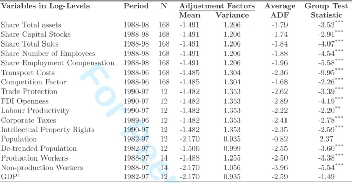
Since the appropriateness of the methodology to be applied to the econometric estimation de-pends on the time series properties of the data, such properties must be ascertained before any estimation is carried out. There are several statistics that may be used to test for a unit root in panel data, but since we have a short-panel data set, we employ the Im, Pesaran and Shin (2003) t-bar statistic, which is based on the mean augmented Dickey-Fuller (ADF) test statistics calculated independently for each cross-section of the panel.
The unavailability of diagnosis tests for the presence of deterministic components in the ADF regressions implies that the unit root tests are carried out using several combinations of deterministic components. In the cases where the results regarding the existence of unit root differ for different models, we pick the model whose deterministic components seem more appropriate when analyzing the plot for each series. Finally, as far as the specification of the test equations is concerned, time dummies are always included to control for common effects across cross-sections.
(Insert table 1 here)
The results of the panel unit root tests for each variable used in this paper are shown in table 1. Since we have annual data with a limited time span, we use one lag to account for autocorrelation. As we may observe in table 1, in every case the null that every variable 8Under trade theory there is an inverse relation between volume of trade and population, as larger countries
tend to be more self-sufficient. On the other hand, there is a direct relation between volume of trade and GDP as it reflects the size of demand and supply of the market.
9GDP could not be included in the present application as it was found to contain a unit root.
3 4 5 6 7 8 9 10 11 12 13 14 15 16 17 18 19 20 21 22 23 24 25 26 27 28 29 30 31 32 33 34 35 36 37 38 39 40 41 42 43 44 45 46 47 48 49 50 51 52 53 54 55 56 57 58 59 60
For Peer Review
contains a unit root for the series in logs is rejected with the exception of GDP and population10.
However, since several empirical studies have shown that population contains a deterministic trend, the unit root test was carried on de–trended population and the null was then rejected.
Having ascertained the time series properties of the data, we now select the variables that are stationary and align the time span pertaining to each variable in order to obtain a balanced panel for all stationary variables. The result is a panel comprising the share of U.S. FDI portrayed in the five measures, transport cost, competition factor, trade barriers index, FDI openness index, labor productivity, corporate taxes, population, intellectual property rights index and production and non-production workers, for the period 1990-1996. With this panel we estimated a share gravity model in order to analyze the determinants of U.S. FDI location.
5
Estimation of the Share Gravity Model
The following dynamic log-linear model, which we call the benchmark model, explains the share of U.S. FDI allocated to each industry in each country of the panel as a function of a set of regressors:
LF SHijtU S = β0LF SHijt−1U S + β1LT Cijt+ β2LCFijt+ β3LT RPit+ β4LF DIOit+
β5LLPit+ β6LCTit+ β7LP OPit+ uijt (7) where i = 1, 2, . . . , 12, denotes countries; j = 1, 2, . . . , 14, denotes industries; t = 2, . . . , 7, denotes periods (years).
The dependent variable, LF SHijt, is the log of the U.S. FDI into industry j of country i over the total FDI outflow from the U.S. into industry j of all countries in the panel at time t.
LT Cijt is the log of the transport costs for industry j between the U.S. parent and its foreign
affiliate in country i at time t. LCFijtis the log of the index that yields the competition factor
faced by industry j in country i at time t. LT RPit and LF DIOit are the logs of the survey
measures of protection to trade and openness to FDI in country i at time t, respectively. LLPit
is the log of labor productivity in country i at time t. LCTit is the log of corporate taxes, and
LP OPit is the log of population in country i, at time t.
The number of observations for each measure of FDI is given by: P12
i=1
14
P
j=1
(Tij − 1) = 1008,
where Tij = T = 7, since we have a balanced panel data. The two-way error component term of
equation (7) is given by:
uijt= λt+ ηi+ ϕj + εijt (8) where ηiaccounts for unobservable country-specific effects, ϕjaccounts for unobservable industry-specific effects and λtaccounts for time-specific effects. The term εijtis the random disturbance
in the regression, varying across time, country and industry cells. As regards the model of equa-tion (7), we assume sequential exogeneity of the regressors, which amounts to postulating that the dynamics of the model are entirely captured by the one-period lagged dependent variable. Thus, the εijtcan be assumed to be independently distributed across individuals with zero mean.
But arbitrary forms of heteroskedasticity across units and time are allowed.
The benchmark model, given by equation (7), will be used primarily to test the validity of the share gravity model as a relevant empirical framework for FDI. Equation (7) provides 10To test for the possibility that the variables which were found to be non-stationary are integrated of second
order, I(2), unit root tests on the first differences of the variables were run. Although not shown here, these tests suggest that all variables are stationary in first differences.
3 4 5 6 7 8 9 10 11 12 13 14 15 16 17 18 19 20 21 22 23 24 25 26 27 28 29 30 31 32 33 34 35 36 37 38 39 40 41 42 43 44 45 46 47 48 49 50 51 52 53 54 55 56 57 58 59 60
For Peer Review
a suitable testing ground for the share gravity model because it groups the variables in (7) so as to match the terms of equation (4). In fact, we can think of transport costs, trade barriers and FDI openness in (7) accounts for the separation term between the source and the target locations, population, labor productivity and corporate taxes can be seen as factors determining the attractiveness of the target location. The remaining two variables in equation (7), competition factor and the lagged dependent variable account for the competition exerted by alternative destinations and the dynamics of the model, respectively. Further ahead, we will add to equation (7) the intellectual property rights index to test the internalization hypothesis and after the number of production and non-production workers to fully test the proximity-concentration hypothesis.
In picking the econometric technique to estimate equation (7) we have to carefully consider the characteristics of this specific panel data. As regards the choice of the estimation procedure, our econometric problem exhibits two defining features. First, we have a typical short-panel, since the number of time periods is limited and the number of units large. This implies that the fixed effects least squares model suggested by M´aty´as (1998) for the estimation of the gravity model, which explicitly estimates the time and individual effects in (8), would result in a large loss of degrees of freedom and quite possibly in multicollinearity problems, since we are estimating extra parameters for the individual and time effects. Second, the presence of the lagged dependent variable in the right-hand side of the regression equation means that the lagged dependent variable is correlated with the unobservable country and industry-specific effects. That is because both LF SHijtU S and LF SHijt−1U S depend on ηi, ϕj, which are imbedded
in the error term. This fact rules out the pooled OLS and the random effects estimators as both estimators would come out inconsistent.
The problem of the correlation between LF SHijt−1US and ηi and ϕj could be overcome by
applying a transformation to the model in equation (7) that would eliminate the unobservable fixed country and industry effects. There two natural such transformations: the within transfor-mation and first-differencing. For the within transfortransfor-mation the
h
LF SHijt−1U S − LF SHU Sij.−1
i will be correlated with [εijt− εij.] even if the random disturbances εijt are not serially correlated,
because LF SHijt−1 is correlated with ¯εij. by construction. For the first-differences transforma-tion the
h
LF SHijt−1U S − LF SHijt−2U S
i
will be correlated with [εijt− εijt−1] even if the random
disturbances εijt are not serially correlated, because LF SHijt is correlated with ¯εijt+1 by
con-struction. In these two cases, the assumption of strict exogeneity is violated, causing both the within and first-differences estimators to be inconsistent.
Under these conditions, especially when estimating dynamic models under short-panel data, Arellano and Bond (1991) suggest exploiting the orthogonality conditions between the explana-tory variables (the lagged dependent variable and the exogenous variables) and the random term that exists in equation (7) in order to instrument the regressors that are correlated with the two-way error component term. Following Arellano and Bond (1991), a GMM estimation procedure is applied to our dynamic panel data model. The standard GMM estimator proposed by Arellano and Bond (1991), which eliminates unobserved specific effects by applying first dif-ferences or orthogonal deviations and taking lagged levels of the regressors as instruments is not suitable for our panel data because the five measures of FDI are found to be highly persis-tent11. Thus, lagged levels are only weakly correlated with subsequent first-differences and as
shown in Blundell and Bond (1998, 1999) in this particular setting, weak instruments can result in large finite-sample biases and imprecision12. If the instruments used in the first-differences
11The results of fitting a AR(1) to all variables considered is available from the authors upon request.
12Blundell and Bond (1998, 1999) demonstrate that the instruments used in the first-difference GMM estimator
become less informative in two important cases: as the value of the autoregressive parameter tends towards unity 3 4 5 6 7 8 9 10 11 12 13 14 15 16 17 18 19 20 21 22 23 24 25 26 27 28 29 30 31 32 33 34 35 36 37 38 39 40 41 42 43 44 45 46 47 48 49 50 51 52 53 54 55 56 57 58 59 60
For Peer Review
estimator are weak, then the first-differences GMM results are expected to be biased down-wards, as with the within groups (see Arellano and Bond, 1991, Blundell and Bond, 1998, 1999). Blundell and Bond (1998, 1999) also showed that biases resulting from using weak instruments could be considerably reduced by incorporating more informative moment conditions. These moments conditions result from using changes in the lags of the regressors as instruments for the equations in levels (Arellano and Bover, 1995). Blundell and Bond (1998) suggest stacking the moments conditions relative to the equations in first-differences and in levels to form what they call the GMM-system estimator. These authors employ Monte Carlo simulations to show that the GMM-system estimator brings about a dramatic improvement in the small-sample bias and precision relative to the standard (Arellano and Bond, 1991) estimator, particularly when the dependent variable is highly persistent (though stationary), which seems to be an essential feature of our data. In view of its superiority in terms of unbiasedness and efficiency, we use the GMM-system estimator in all estimations of the share gravity model.
In the context of our share gravity model, the precise set of instruments that give rise to the moment conditions depends on the degree of exogeneity we are prepared to assume for the regressors other than the lagged dependent variable. As we do not expect all regressors to be strictly exogenous, we assume sequential exogeneity as we did for the lagged dependent variable. This leads to moments conditions that imply that the residuals of the estimated equations are uncorrelated with contemporaneous and past observations of all the regressors. Therefore, the matrix of instruments is composed of lagged levels of the dependent variable dated t − 2 and earlier and lagged levels of the remaining regressors dated t − 1 and earlier in the first difference equations and of lagged differences of the dependent variable dated t − 2 with lagged first-differences of the remaining regressors dated t − 1 as instruments in the levels equations.
5.1 Estimation Results
The results pertaining to the estimation of the benchmark share gravity model in (7) as well as some extensions to it are reported in tables 2, 3 and 4. In table 2 we report the results found for each of the five measures of FDI. Moreover, since the various measures of FDI are likely to be highly correlated, we used the principal component analysis (PCA) to analyze the underlying dimensionality of the five measures. The five eigenvalues were 4.636, 0.306, 0.034, 0.019 and 0.006. Since the largest eigenvalue accounts for 92.7 per cent of the total variation and the corresponding eigenvector suggests that all variables have nearly the same weight, we may conclude that any of the five measures of FDI may be used to picture the FDI phenomenon, or that the effective dimensionality of the FDI data is one. In other words, the estimation results should be almost identical for each of the five measures. A new series, PCV, was created using the first principal component. As patent in table 2, the econometric results seem to be consistent with the PCA predictions. Thus, in tables 3 and 4 we report only the results for the PCV variable.
In all tables 2, 3 and 4 we report the results for both the one-step and two-step GMM-system estimators. The one-step estimator uses a weighting matrix that is independent of estimated parameters, while the (asymptotically) more efficient two-step estimator uses a weighting matrix that corresponds to the variance matrix of the estimated residuals of the one-step estimator. In spite of its asymptotic higher efficiency relative to the one-step estimator, the two-step estimator produces downward biased variance estimates in small samples due to the extra variation intro-duced by the presence of estimated parameters rather than the true ones, resulting in oversized individual and joint significance tests. In this context, it has been advocated the use of the one-step estimator for inference, since this estimator reports a dispersion around the point estimate and as the variance of the fixed effects increases relative to the variance of the random shocks.
3 4 5 6 7 8 9 10 11 12 13 14 15 16 17 18 19 20 21 22 23 24 25 26 27 28 29 30 31 32 33 34 35 36 37 38 39 40 41 42 43 44 45 46 47 48 49 50 51 52 53 54 55 56 57 58 59 60
For Peer Review
that is closer to the asymptotic one in finite samples. In any case, the trade-off between the higher asymptotic efficiency and the downward biasedness of the variance estimates pertaining to the two-step GMM-system estimator hinges, in a rather complex way, on the specific model in hand, the number of cross-section and time periods, the specific instruments used, and the num-ber of moments. Therefore, the choice between the one-step and the two-step GMM estimators for the analysis of the results is not straightforward.
Along with the estimated coefficients of the share gravity model and the respective p-values, we report several specification tests. The Wald test evaluates the overall significance of the model under the null hypothesis that all coefficients are jointly zero. We also report a first-order and second-order autocorrelation tests for the residuals of the equations in first-differences. The rationale for this is that the presence of serial correlation in the residuals of the original model (in levels) constitutes evidence that sequential exogeneity of the regressors cannot hold, which in turn implies the invalidity of moment conditions that rely on the levels (or changes) of lags of the dependent variable as instruments, as it is the case with the GMM-system estimator we are using. Since we are testing for autocorrelation of the residuals in the differenced equations, we should expect to find first-order serial correlation but no evidence of second-order autocorrelation if the model is well specified, i.e. if our specification fully captures the dynamics of the underlying true model13. Finally, we report a Sargan test for the overidentifying restrictions under the null of the validity of the moment conditions.
In table 2, for both one-step and two-step GMM-system estimators we reject the null of the Wald test and so accept the overall significance of the regressors. We fail to reject first-order but not second-order autocorrelation of the residuals in the equations in first-differences, which constitutes evidence in favor of the validity of the assumption of sequential exogeneity. Even though there is a strong tendency for the Sargan test to over-reject the null hypothesis under the presence of heteroskedastic errors, the validity of the over-identifying restrictions are not rejected for TA, KS and PCV. A model with an intercept was estimated and, as expected, the intercept turned out to be statistically insignificant, since the dependent variable is expressed in shares, not levels. It turns out that the model in equation (7) seems to be well specified and to explain the share of FDI reasonably well. Moreover, the estimated individual coefficients for the various measures of FDI were generally found to have the correct sign and to be statistically significant (at least for the two-step GMM estimator). Adding to all this the fact that the competition factor, which is absent from the classical version, has been estimated to have a detrimental effect on the share of FDI, not only vindicates the share gravity model as a suitable framework for the analysis of the locational determinants of FDI, but is also suggestive of its superiority over the classical version.
The results of the estimation of equation (7) suggest that the share of FDI exhibits a high persistence as the coefficient on the lagged dependent variable was found to be relatively close to one and quite significant. As often contended in the literature, this can be regarded as evidence in favor of the presence of agglomeration effects in FDI.
(Insert table 2 here)
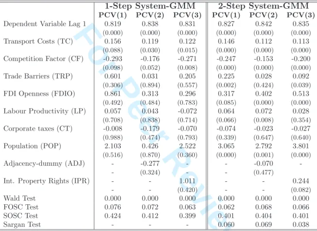
The inclusion of an adjacency dummy and of intellectual property rights (IPR) variable is assessed in the share gravity model by using the PCV measure of FDI (see table 3). The adjacency dummy takes the value of one for Mexico and Canada and zero otherwise. The effects of adjacency are generally analyzed in light of the impact of the geographical proximity on FDI decisions. However, in the particular case of the U.S., the two adjacent countries form with the
13If a series u
tare iid it can be easily shown that corr(∆ut, ∆ut−1) = −0.5 and corr(∆ut, ∆ut−2) = 0. 3 4 5 6 7 8 9 10 11 12 13 14 15 16 17 18 19 20 21 22 23 24 25 26 27 28 29 30 31 32 33 34 35 36 37 38 39 40 41 42 43 44 45 46 47 48 49 50 51 52 53 54 55 56 57 58 59 60
For Peer Review
U.S. a trade zone (NAFTA), which leads us also to consider the effects of regional integration on FDI when looking at the estimated effects of adjacency.
According to the “distance-incentive” concept, which assumes higher relevance for horizontal FDI, the adjacency parameter estimate should be negative as low transport costs should render exporting more advantageous than FDI. However, adjacency also exerts some positive effects on the potential to attract FDI, as it may encourage local production destined to be exported back to the parent firm’s home market or MNEs’ vertical integration across borders (Brainard, 1993a) and also reduce the cost of supervision of foreign affiliates (Ethier and Horn, 1990, Lipsey, 1999, 2000). The results are presented in table 3. It appears that, if anything, adjacency plays an overall negative role in the location of FDI (see columns PCV(2) for both the one-step and two-step estimators in table 3). The lack of statistical significance of the estimated coefficient on adjacency might be reflecting the fact that we would expect the FDI flowing to Mexico to be predominantly of the vertical type and that flowing to Canada to be predominantly of the horizontal type. Therefore, since these two types of FDI are affected by distance in opposite ways, the positive effect of adjacency pertaining to Mexico might be canceling out the negative effect pertaining to Canada. These conflicting effects will further interact with the also potentially contradictory effects of NAFTA on American FDI (see section 1). Overall, the lack of a discernible impact of adjacency on U.S. FDI is perfectly compatible with the predictions of the FDI theory.
The columns PCV(3) for both the one-step and two-step estimators in table 3 show the results of the share gravity model with the inclusion of the IP R variable. The estimated coefficient of
IP R measures how keen MNEs are in protecting their proprietary advantages. The coefficient
on IP R appears positive as expected, though not significant under the one-step estimator. This implies that MNEs will, ceteris paribus, invest in the locations that better guarantee that their know-how cannot be improperly exploited by local competitors, which conforms with the “internalization” hypothesis.
(Insert table 3 here)
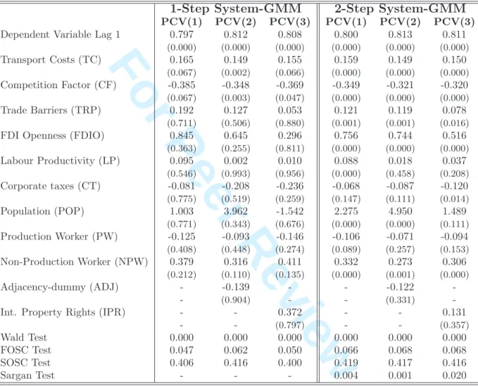
Finally, we test the “proximity-concentration” hypothesis using the share gravity model. Since we use shares of FDI allocated to each country in the panel, we are controlling for the determinants of trade flows that are common to all alternative locations in the panel thereby mitigating the potential problems associated with the joint determinacy of exports and FDI. The results of including the scale-economies variables in the original share gravity model (equation 7) are reported in the columns PCV(1) for both the one-step and two-step estimators in table 4. All the coefficients have the predicted sign. Specifically, in regard to the scale variables, the coefficient on production workers (P W ) is negative and significant at 10 percent under the two-step estimator but not significant under the one-step estimator. The non-production workers’ (N P W ) coefficient is positive and significant. Hence, scale economies at the plant level, by which the concentration of production lowers unit costs, affect negatively the share of FDI allocated to each country in the panel. On the other hand, scale economies at the corporate level, which imply that the firm has an input that can be spread among any number of factories with undiminished value, affects positively the share of FDI. This combined with the positive effect of transport costs, trade barriers and of market size, indicates that the share of FDI allocated to each country in the panel is an increasing function of proximity advantages but decreasing in the advantages from concentrating production in one location.
Comparing these results with the ones of the column PCV(1) of the two-step estimator dis-played in table 3, the elasticities given by the coefficients of CF and FDIO are significantly higher under the “proximity-concentration” hypothesis. Thus, the weight of competition of potential
3 4 5 6 7 8 9 10 11 12 13 14 15 16 17 18 19 20 21 22 23 24 25 26 27 28 29 30 31 32 33 34 35 36 37 38 39 40 41 42 43 44 45 46 47 48 49 50 51 52 53 54 55 56 57 58 59 60
For Peer Review
competing countries and the host market investment climate comes stronger in equations where the firm is assumed to be confronted with the trade-off between proximity to consumers and concentration of production. In sum, the “proximity-concentration” hypothesis is not rejected when explaining the share of FDI allocated to each country in the panel. All relevant variables appear with the correct sign, namely corporate scale economies and production scale economies are positive and negatively, respectively, related to the share allocated to a specific location. Again adjacency and IP R have the predicted signs.
(Insert table 4 here)
6
Conclusion
The effect of several factors on the location of FDI is tested under the share gravity model using panel data on U.S. MNEs disaggregated at the industry level. The share of U.S. FDI, portrayed by five different measures, is increasing in lagged FDI shares, transport costs, trade barriers, FDI openness, labor productivity and population, and decreasing in competition posed by other countries and corporate taxes. This evidence suggests that country-specific locational factors are very important determinants of the U.S. FDI. These results combined with the fact that the factor capturing the gravity of the competing destinations emerges very significant and with the correct sign across the different measures of FDI vindicates the use of the share formulation of the gravity model to the analysis of the location of MNEs’ activities.
The share of U.S. FDI is also increasing in the level of protection of intellectual property rights (IPR) in the host country. Thus, when there are intellectual property advantages, as as-sumed by the imperfect competition models of multinationals, which are easily transferred across borders, MNEs will choose the countries that better protect those advantages. The “proximity-concentration” hypothesis is not rejected when explaining the share of FDI allocated to each country in the panel. All relevant variables appear with the correct sign, namely corporate scale economies and production scale economies are respectively, positive and negatively related to the share allocated to a specific location.
Acknowledgements
I am grateful to Jim Ford, Peter Burridge and Manuel Arellano. An early version of this paper has also benefited from presentations at the 11th Panel data Conference in Texas, USA, 11th
Conference of Dynamics, Economic Growth and International Trade, in Jerusalem, Israel and 21th Annual Congress of the European Economic Association 2006, in Vienna, Austria.
3 4 5 6 7 8 9 10 11 12 13 14 15 16 17 18 19 20 21 22 23 24 25 26 27 28 29 30 31 32 33 34 35 36 37 38 39 40 41 42 43 44 45 46 47 48 49 50 51 52 53 54 55 56 57 58 59 60
For Peer Review
References
Anderson, J. E. and Wincoop, E. V. (2003), ‘Gravity with gravitas: A solution to the border puzzle’, American Economic Review .
Arellano, M. and Bond, S. (1991), ‘Some tests of specification for panel data: Monte Carlo evidence and an application to employment equations’, Review of Economic Studies 58, 277– 297.
Arellano, M. and Bover, O. (1995), ‘Another look at the instrumental-variable estimation of error-component models’, Journal of Econometrics 68, 29–52.
Bergstrand, J. H. (1985), ‘The gravity equation in international trade: Some microeconomic foundations and empirical evidence’, Review of Economics and Statistics 67, 474–481. Bergstrand, J. H. (1989), ‘The generalized gravity equation, monopolistic competition, and the
factor-proportions theory in international trade’, Review of Economics and Statistics 71, 143– 153.
Bergstrand, J. H. (1990), ‘The heckscher-Ohlin-Samuelson model, the Linder hypothesis and the determinants of bilateral intra-industry trade’, The Economic Journal 67, 1216–1229. Blomstrom, M. and Kokko, A. (1997), Regional integration and Foreign direct investment,
Working Paper 6019, National Bureau of Economic Analysis.
Blonigen, B. A. (2005), ‘A review of the empirical literature on FDI determinants’, Atlantic
Economic Journal 33, 383–403.
Blundell, R. and Bond, S. (1998), ‘Initial conditions and moment restrictions in dynamic panel data models’, Journal of Econometrics 87, 115–143.
Blundell, R. and Bond, S. (1999), GMM estimation with persistent panel data: An application to production Functions, Working Paper Series W99/4, The Institute for Fiscal Studies. Brainard, S. L. (1993a), An empirical assessment of the factor proportions explanation of
multi-national sales, Working Paper 4583, National Bureau of Economic Research.
Brainard, S. L. (1993b), A simple theory of multinational corporations and trade with a trade-off between proximity and concentration, Working Paper 4269, National Bureau of Economic Research.
Brainard, S. L. (1997), ‘An empirical assessment of the proximity-concentration trade-off be-tween multinational sales and trade’, American Economic Review 87, 520–544.
Carr, D., Markusen, J. R. and Markus, K. E. (2001), ‘Estimating the knowledge-capital model of the multinational enterprize’, American Economic Review .
Caves, R. E. (1974), ‘Causes of direct investment: Foreign firms’ shares in canadian and united kingdom manufacturing industries’, The Review of Economic and Statistics 56, 279–293. Caves, R. E. (1996), Multinational Enterprise and Economic Analysis, Cambridge Surveys of
Economic Literature, Cambridge University Press, Cambridge, U.K.
Cheng, L. K. and Kwan, Y. K. (2000), ‘What are the determinants of the location of foreign direct investment? the Chinese experience’, Journal of International Economics 51, 379–400.
3 4 5 6 7 8 9 10 11 12 13 14 15 16 17 18 19 20 21 22 23 24 25 26 27 28 29 30 31 32 33 34 35 36 37 38 39 40 41 42 43 44 45 46 47 48 49 50 51 52 53 54 55 56 57 58 59 60
For Peer Review
Cushman, D. O. (1987), ‘The effects of real wages and labour productivity on foreign direct investment’, Southern Economic Journal 54, 174–185.
de Mello-Sampayo, F. (2006), ‘The location of United States FDI under the share gravity model’,
International Economics Journal, forthcoming .
Dunning, J. H. (1988), Explaining International Production, Harper Collins, London, UK. Dunning, J. H. (1993), Multinational Enterprises and the Global Economy, Addison-Wesley
Publishers Ltd.
Ekholm, K., Forslid, R. and Markusen, J. R. (2006), Export–platform foreign direct investment, Working Paper 9517, National Bureau of Economic Research.
Ethier, W. J. (1986), ‘The multinational firm’, Quarterly Journal of Economics 101, 805–833. Ethier, W. J. and Horn, H. (1990), ‘Managerial control of international firms and patterns of
direct investment’, Journal of International Economics 28, 25–45.
Ethier, W. J. and Markusen, J. R. (1996), ‘Multinational firms, technology diffusion and trade’,
Journal of International Economics 41, 1–28.
Fotheringham, A. S. (1983a), ‘A new set of spatial-interaction models: The theory of competing destinations’, Environment and Planning A 15, 15–36.
Fotheringham, A. S. (1983b), ‘Some theoretical aspects of destination choice and their relevance for production-constraint gravity models’, Environment and Planning A 15, 1121–1132. Fotheringham, A. S. (1984), ‘Spatial flows and spatial patterns’, Environment and Planning A
16, 529–542.
Grubbert, H. and Mutti, J. (1991), ‘Taxes, tariffs and transfer pricing in multinational corporate decision making’, Review of Economics and Statistics 73, 285–293.
Harrigan, J. (1993), ‘OECD imports and trade barriers in 1983’, Journal of International
Eco-nomics 35, 91–111.
Haufler, A. and Wooton, I. (1997), Tax competition for Foreign direct investment, Discussion Paper 1583, Centre for Economic Policy Research.
Head, K., Ries, J. and Swenson, D. (1995), ‘Agglomeration benefits and location choice: Ev-idence from Japanese manufacturing investments in the United States’, Journal of
Interna-tional Economics 38, 223–247.
Helpman, E. (1984), ‘A simple theory of international trade with multinational corporations’,
Journal of Political Economy 92, 451–471.
Helpman, E. (2006), Trade, FDI, and the organization of firms, Working Paper 12091, National Bureau of Economic Research.
Helpman, E. and Krugman, P. R. (1985), Market Structure and Foreign Trade, The MIT Press, Cambridge, Massachussets.
Horst, T. (1972a), ‘Firm and industry determinants of the decision to invest abroad: An empir-ical study’, Review of Economics and Statistics 54, 258–266.
3 4 5 6 7 8 9 10 11 12 13 14 15 16 17 18 19 20 21 22 23 24 25 26 27 28 29 30 31 32 33 34 35 36 37 38 39 40 41 42 43 44 45 46 47 48 49 50 51 52 53 54 55 56 57 58 59 60
For Peer Review
Horst, T. (1972b), ‘The industrial composition of US exports and subsidiary sales to the canadian market’, American Economic Review 62, 37–45.
Horstmann, I. and Markusen, J. R. (1987), ‘Licensing versus direct investment: A model of internationalization by the multinational enterprise’, Canadian Journal of Economics 20, 464– 481.
Horstmann, I. and Markusen, J. R. (1992), ‘Endogenous market structures in international trade (natura facit saltum)’, Journal of International Economics 32, 109–129.
Hua, C. and Porell, F. (1979), ‘A critical review of the development of the gravity model’,
International Regional Science Review 4, 97–126.
Im, K. S., Pesaran, M. H. and Shin, Y. (2003), ‘Testing for unit roots in heterogeneous panels’,
Journal of Econometrics 115, 53–74.
Kau, J. B. and Sirmans, C. F. (1979), ‘The functional form of the gravity model’, International
Regional Science Review 4, 127–136.
Krugman, P. R. (1980), ‘Scale economies, product differentiation, and the pattern of trade’,
American Economic Review 70, 950–959.
Krugman, P. R. (1983), The “New Theories” of International Trade and the Multinational
Enterprise, The MIT Press, Cambridge, Massachussets, pp. 57–73.
Linnemann, H. (1961), An Economic Study of International Trade Flows, North-Holland, Ams-terdam, Netherlands.
Lipsey, R. E. (1999), The location and characteristics of US affiliates in asia, Working Paper 6879, National Bureau of Economic Research.
Lipsey, R. E. (2000), Interpreting developed countries’ foreign direct investment, Working Paper 7810, National Bureau of Economic Research.
Markusen, J. R. (1984), ‘Multinationals, multi-plant economies and the gains from trade’,
Jour-nal of InternaioJour-nal Economics 16, 205–226.
Markusen, J. R. (2002), Multinational Firms and the Theory of International Trade, The MIT Press, Cambridge, Massachussets.
Markusen, J. R. and Venables, A. (1996), The theory of endowment, intra-industry trade, and multinational trade, Discussion Paper 1341, Centre for Economic Policy Research.
Masahisa Fujita, P. K. and Venables, A. J. (1999), The Spatial Economy: Cities, Regions, and
International Trade, Massachusetts Institute of Technology, United States of America.
M´aty´as, L. (1998), ‘The gravity model: Some econometric considerations’, World Economy 21, 397–401.
Roy, J. R. (2004), Spatial Interaction Modelling: A regional Science Context, Springer–Verlag, Berlin Heidelberg New York.
Thorsen, I. and Gitlesen, J. P. (1998), ‘Empirical evaluation of alternative model specifications to predict commuting Flows’, Journal of Regional Science 38, 272–292.
Wheeler, D. and Mody, A. (1992), ‘International investment location decisions’, Journal of
International Economics 33, 57–76. 3 4 5 6 7 8 9 10 11 12 13 14 15 16 17 18 19 20 21 22 23 24 25 26 27 28 29 30 31 32 33 34 35 36 37 38 39 40 41 42 43 44 45 46 47 48 49 50 51 52 53 54 55 56 57 58 59 60
For Peer Review
Appendix
A
List of Industries
I1 - All industries
I2 - Petroleum I10 - Other manufacturing
Oil and gas extraction Tobacco products
Crude petroleum extraction (no refining) and natural gas Textile products and apparel
Oil and gas field services Lumber, wood, furniture, and fixtures
Petroleum and coal products Paper and allied products
Integrated petroleum refining and extraction Printing and publishing
Petroleum refining without extraction Rubber products
Petroleum and coal products, nec Miscellaneous plastics products
Petroleum wholesale trade Glass products
Other Stone, clay, and other nonmetallic mineral products
Instruments and related products
I3 - Manufacturing Other
I4 - Food and kindred products I11 - Wholesale trade
Grain mill and bakery products Durable goods
Beverages Nondurable goods
Other
I12 - Finance (except banking) ,
insurance, and real estate
I5 - Chemicals and allied products Finance, except banking
Industrial chemicals and synthetics Insurance
Drugs Real estate
Soap, cleaners, and toilet goods Holding companies
Agricultural chemicals
Chemical products, nec I13 - Services
Hotels and other lodging places
I6 - Primary and fabricated metals Business services
Primary metal industries Advertising
Ferrous Equipment rental (ex automotive and computers)
Nonferrous Computer and data processing services
Fabricated metal products Business services, nec
Automotive rental and leasing
I7 - Machinery, except electrical Motion pictures, including television tape and film
Farm and garden machinery Health services
Construction, mining, and materials handling machinery Engineering, architectural, and surveying services
Office and computing machines Management and public relations services
Other Other
I8 - Electric and electronic equipment I14 - Other industries
Household appliances Agriculture, forestry, and fishing
Radio, television, and communication equipment Mining
Electronic components and accessories Metal mining
Electrical machinery, nec Nonmetallic minerals
Construction
I9 - Transport equipment Transport
Motor vehicles and equipment Communication and public utilities
Other Retail trade
3 4 5 6 7 8 9 10 11 12 13 14 15 16 17 18 19 20 21 22 23 24 25 26 27 28 29 30 31 32 33 34 35 36 37 38 39 40 41 42 43 44 45 46 47 48 49 50 51 52 53 54 55 56 57 58 59 60