Three-Gorges Dam Fine Sediment Pollutant Transport: Turbulence SPH Model Simulation of Multi-Fluid Flows

Journal of Applied Fluid Mechanics, Vol. 9, No. 1, pp. 1-10, 2016.

Available online at www.jafmonline.net, ISSN 1735-3572, EISSN 1735-3645.

Three-Gorges Dam Fine Sediment Pollutant Transport:

Turbulence SPH Model Simulation of

Multi-Fluid Flows

J. H. Pu

1†

, Y. Huang

2

, S. Shao

3

and K. Hussain

1

1 _{School of Engineering, Faculty of Engineering and Informatics, University of Bradford, Bradford BD7 1DP,}

UK

2 _{State Key Laboratory of Hydro-Science and Engineering, Tsinghua University, Beijing 100084, China} 3 _{Department of Civil and Structural Engineering, University of Sheffield, Sheffield S1 3JD, UK}

†Corresponding Author Email: j.h.pu1@bradford.ac.uk

(Received July 7, 2014; accepted November 10, 2014)

ABSTRACT

The Three Gorges Dam (TGD) constructed at the Yangtze River, China represents a revolutionary project to battle against the mage-scale flooding problems while improving the local economy at the same time. However, the large-scale fine-size sediment and pollutant material transport caused by the TGD operation are found to be inevitable and long-lasting. In this paper, a multi-fluid Incompressible Smoothed Particle Hydrodynamics (ISPH) model is used to simulate the multi-fluid flows similar to the fine sediment materials transport (in muddy flows) and water flow mixing process. The SPH method is a mesh-free particle modeling approach that can treat the free surfaces and multi-interfaces in a straightforward manner. The proposed model is based on the universal multi-fluid flow equations and a unified pressure equation is used to account for the interaction arising from the different fluid components. A Sub-Particle-Scale (SPS) turbulence model is included to address the turbulence effect generated during the flow process. The proposed model is used to investigate two cases of multi-fluid flows generated from the polluted flow intrusions into another fluid. The computations are found in good agreement with the practical situations. Sensitivity studies have also been carried out to evaluate the particle spatial resolution and turbulence modeling on the flow simulations. The proposed ISPH model could provide a promising tool to study the practical multi-fluid flows in the TGD operation environment.

Keywords: Three gorges dam; Pollutant transport; Density difference; SPH; Multi-fluid; Fine sediment.

1.

INTRODUCTION

With the investment in construction and resettlement of approximate USD 29 billions, the key goals of the Three Gorges Dam (TGD) project are to: 1) control the floods; 2) generate the electric power; and 3) improve the navigation at the Yangtze River (United Nations, 2014). The TGD’s floods control mainly concentrates on protecting the mid to downstream of the Yangtze River, in which numerous devastating floods had happened, e.g. the floods in 1954 and 1998 that claimed many lives and caused millions of people

being relocated (Yang et al., 2009).In terms of the

hydropower generation, the TGD is expected to generate about 84.7 TWh/yr (terawatt-hour per year) following the feasibility study, while the actual production was about 100 TWh/yr in 2011 (UC, 2012). Besides, the TGD project also aims to improve the navigation between two important

ports: Shanghai and Chongqing, where the cargo transport throughout the Yangtze River ports has increased from 400 million tons in year 2000 to nearly 1.2 billion tons in year 2008, surpassing the Rhine in Europe and Mississippi in USA to place itself on the top world ranking for four consecutive years in terms of the world-wide

inland freight haulage (Yang et al., 2009; United

Nations, 2014).

The idea of TGD project started in 1994, the initial impoundment of the Three Gorges Reservoir happened in 2003 and the project was fully completed in 2010. The TGD is 181 m high and its designed flood control level is 145 m, but the concrete gravity dam has been found to withstand a normal pool water level of 175 m on 26 October 2010 (UC, 2012). The reservoir stores

approximately 39.3 billion m3 water with a

coverage area of 1084 km2. Approximately 27

managed by the TGD during the 2010 flood. In terms of flooding control, the TGD is designed for managing the 1000-year flood event with a capacity

of around 0.11 million m3/s, but this design capacity

has only been so far tested by the 2011 flood in the lower Yangtze River corresponding to the 100-year

flood event (United Nations, 2014).

As outlined in Guo (2010) and Subklew et al.

(2010), even though the TGD project provides a lot of benefits to improve the flood protection and local economy, its environmental and social impacts could be long lasting and massive. This statement

has been agreed by Xu et al. (2013) who

investigated the environmental impacts caused by the TGD through looking into several key factors, such as the reservoir sedimentation and downstream riverbed erosion, soil erosion, seismic activity and geological hazard, and water quality. It was recorded since the initial impoundment within 2003-2006, the maximum bed elevation changes in the downstream region of the TGD at Jingjiang River reached 13 m, which exceeded the original feasibility study of 5-7 m. This is believed to be directly caused by the TGD water storage that only allows the limited water to flow through the downstream and hence create an unhealthy flow conditions to flash the eroded materials away. The situation in the downstream area coupled with the sediment discharge from the TGD led to a sharp increase in the sediment volume, e.g. the fine sediment pollutants and eroded materials from Yichang to Chenglingji were recorded to be 330

million m3 _{between October 2003 and October}

2007. This could be equal to 61.4 % of the total

erosion volume in the Yangtze River (Yang et al.,

2009). Thus it is not difficult to foresee that with the continuous operation of the TGD, the sediment pollutant level will continue to deteriorate in the downstream region for a long period of time.

In October 2010, the sediment inflow to the TGD was recorded to be more than the outflow by

around 200 million m3_{, and also the sediment}

materials in the downstream area were in significantly fine size of around 4 μm – almost entirely silt clay (UC, 2012). With the existence of the silt clay and water flow mixtures (mixed muddy flows), it can generate similar flow condition to the lock exchange multi-fluid flows that can damage the turbines and cause inefficient power generations. It was analyzed from the sediment budget in the Three Gorges Reservoir from 2003 to 2010 that about 172 million ton/year was captured in the reservoir, which is equivalent to the trapping of 78% of the inflow sediment (UC

2012; Xu et al. 2013). As a consequence, more

than 50 meters high of the deposited sediment materials have been built up in the wide areas near the reservoir (UC 2012). Hence the lock-exchange multi-fluid flows (between the denser muddy flow and lighter water flow) should be extensively studied to understand their effect on the TGD operation and identify possible plans to reduce the hazard from sediment transport.

By definition, the lock exchange flow (also known

as gravity flow) is the flow of a fluid with heavier density (muddy flow) intruding into another fluid with a lighter density (water medium) under the influence of the gravity. The density difference in fluids can be due to the difference in the material and temperature, also could be due to the dissolutions of particular matters such as the saline and sediment in our present study. The gravity flow is widely found in the environmental and hydraulic applications and thus the investigation of this flow has a significant theoretical and practical importance. In the early studies, many researchers used the analytical and experimental approaches to gain basic understandings of the flow dynamics and structures. Some excellent reviews of the previous

works can be found in Monaghan et al. (1999;

2009).

Numerical simulations based on the Navier-Stokes (N-S) equations can provide a good approach to study the TGD induced gravity current flows due to its cost-effectiveness as compared with the physical experiments or field surveys. The N-S modeling can calculate the multi-density flows under very complicated conditions to disclose the detailed flow information about the interface deformation, velocity structure, transport, extensive mixing and entrainment process. Recently the numerical solution schemes of using mesh-free particle modeling technique have become a promising trend that is vigorously explored by a lot of researchers. In a particle model, the governing equations are discretized and solved by the individual particles that fill in the computational domain. The particle interaction models are used to treat all the terms in the hydrodynamic equations. Compared with the grid modeling approach, the particle model has the advantages to track the free surfaces and multi-interfaces in an easy and accurate manner without numerical diffusion, so as to make it a useful tool for the study of the multi-fluid flows, such as the TGD lock exchange gravity flows in this study. The Smoothed Particle Hydrodynamics (SPH) method is one highly robust particle modeling technique that was originally developed for the astrophysical flows (Monaghan, 1992) and afterwards was modified for the incompressible free surface flows, including some multi-fluid flows such as the dust gas flow (Monaghan and Kocharyan, 1995), gravity current flow

(Monaghan et al., 1999), water-air interfacial flow

(Colagrossi and Landrini, 2003) and muddy flow (Ataie-Ashtiani and Shobeyri, 2008).

2013), the current work focuses more on the influence of turbulence modeling and pressure analysis aiming to validate the commonly adopted practice of using the inviscid modeling/shallow water (SW) approaches to model such gravity flows

(such as in Pu et al. (2012)). The flow turbulence is

modeled based on the concept of the Sub-Particle Scale (SPS) turbulence approach originally

proposed by Gotoh et al. (2001) for the turbulence

jet.

2.

MOTIVATIONS OF STUDY

According to the relevant TGD authorities, the primary reason of building the TGD was to control the frequent and devastating floods in the middle and lower reaches of the Yangtze River. Besides, the dam can also produce costless and clean electric power to the energy-required regions (mainly in the Central and East China). However, some environmental impacts from the pollutant migration contributed to the adverse effect on the original building purposes (Chinese Government State Council 2011).

By looking at the mechanisms of the flood-control and power generation, one of the most crucial factors could come from the lock exchange flows in the downstream dam area. This lock exchange flow is due to the various sources, such as the heavy metal or sedimentation mixture with the water, or temperature difference. These have caused the flood control capacity being reduced and also given rise to various social problems. To fully understand the fundamental flow process, physical experiments and field studies have been used but they are usually constrained by the practical situations and measurement limitations. Thus computer simulations have become a very crucial strategy to understand the dam operation process and the related sediment pollutant migration. In this study, we attempt to use an advanced SPH model to simulate the lock-exchange flows aiming to help the TGD planning and sediment management. The purpose of this study is to find out the exchange characteristics of different fluids when a heavier pollutant flow mixes with the lighter one. This could effectively give us an indication of how the sediment pollutants will migrate so as to study possible defensive measures to battle against the sediment pollution issues caused by the dam construction and operation.

The following sections will look into the numerical SPH model. The full governing equations together with the numerical solution schemes will be discussed. Fundamental assumptions used in the modeling approach as well as necessary boundary conditions will also be explored to understand the limitation and advancement of the proposed approach. Lastly, we will apply the SPH model to two artificially created environments to investigate the sediment pollutant migration using the lock exchange flows. This computational study should provide us with the necessary information about the potential issues of the sediment pollutant transport

in the TGD area.

3.

MULTI-FLUID SPH MODEL WITH

TURBULENCE

3.1

Governing Equations

The proposed multi-fluid SPH model is established based on the general multi-phase flow equations. In a particle modeling approach, the mass and momentum equations for a two-fluid flow system are represented in the Lagrangian form as follows:

1

u 0

1

u 0

l l l

s s s

d dt d

dt

 

 



   _{ }

  

   



(1)

2

2

u

g u f

u

g u f

l

l l l l l ls

s

s s s s s ls

d P dt d

P dt

  

  



      _

 

     



(2)

in which  = density; t = time; u = velocity; P =

pressure; g = gravitational acceleration;  =

dynamic viscosity; and f = interaction forces

among the different fluid components. The

subscript l and s refers to the different fluid

components.

3.2

Numerical Solution Schemes

The incompressible SPH solution process employs a two-step prediction/correction approach to solve the governing equations (1) and (2). The final flow velocity is calculated by using a time-marching procedure as:

* **

, 1 , , ,

u_{m t} u_{m t} u_{m t} u_{m t}

(ml s, )

(3)

in which u*m t, = velocity increment in the

prediction step; u**_{m t,} = velocity increment in the

correction step; um t_, = velocity at time t; and

1 ,t m

u = velocity at time t1. Here ml s, refer

to the different fluid components.

The prediction step in the solution procedures is an explicit integration in the time without enforcing the fluid incompressibility. In this step, only the gravitational and viscous forces in equation (2) are used and an intermediate particle velocity and position of the flow are obtained as

* 2

,

u_{m t} ( m u )_{m t} g

m

t t

 

      (4)

* *

, , ,

* *

, , ,

u u u

r r u

m t m t m t

m t m t m t t



   _



  _{ } (ml s, ) (5)

in which t = time increment; rm t, = particle

position at time t; and r_{m t}*_, = intermediate particle position.

This is manifested by the fact that the intermediate

density of the fluid particles _* _{deviated from the}

initial constant density _0_{. Thus the densities of the}

particles are required to be corrected to their initial values in the correction step to re-satisfy the incompressibility. The particle velocity increment in the correction step is calculated by

**

, , 1 ,

**

, , 1 ,

u f

u f

l l t l t ls t

s s t s t ls t

P t t

P t t

          _{ } 

     _{ }

(6)

By adding the above two equations together and following Gotoh and Sakai (2006), the interaction terms can be eliminated and included in the pressure term. A general unified pressure Poisson equation can be derived through the continuity condition as

0 *

1 0 2

1 ( ) ( ) t m P t          

 (ml s, )

(7) By using the above pressure equation, the calculation of velocity increment in equation (6) can be simplified and the unknown particle interaction forces are dropped as represented below

** , 1 ** , 1 u u

l l t t

s s t t

P t P t         _{ } 

   _{ }

(8)

Finally, the spatial position of the fluid particle is calculated by using a central scheme in the time as:

, , 1

, 1 ,

(u u )

r r

2

m t m t

m t m t t



     (ml s, ) (9)

in which

r

_m,t1 = position of the particle at time

1 

t . It should be mentioned here that as the

present SPH model uses equation (7) to compute the fluid pressure through a semi-implicit approach, it is called as incompressible SPH – ISPH model.

3.3

Basic SPH Formulations

In an SPH computation, the modeled fluid media are discretized as an assembly of a large number of individual particles. The particle interaction zone is supposed to be around each particle. All of the terms in the governing equations (1) and (2) are described as the interactions between the reference particle and its neighbors. Thus the computational grid is not required. Combined with adequate initial and boundary conditions, any hydrodynamic problem can be solved exclusively through the particles. The detailed reviews of the SPH principle are summarized by Monaghan (1992). The following standard SPH formulations are used in the present model.

For example, the density of a fluid particle a is

calculated by

( r r , )

a b a b

b

m W h

 



 (10)

in which a and b = reference particle and its

neighbors; m_b = particle mass; r_a and r_b = particle

positions; W = interpolation kernel and h =

smoothing distance. The pressure gradient uses an anti-symmetric form as:

2 2

1

( )a b( a b) a ab

b a b

P P

P m W

 



  

(11)

in which the summation is over all the particles

other than particle a and _aW_ab = gradient of the

kernel taken with respect to the position of particle

a. The Laplacian in the pressure term and the

laminar viscosity are formulated as a hybrid of a standard SPH first derivative combined with a finite difference approximation for the first derivative. The purpose is to eliminate the numerical instability caused by the particle disorders arising from the second derivative of the kernel

2 2

( )(r r )

1 8

( )

( ) r r

a b a b a ab

a b

b a b a b

P P W

P m             



(12) 2 2 2( )

(u u )(r r )

( u)

r r

a b

a b a b a b a ab

a b

a b

b a b

W m                _



(13)

3.4 Turbulence Modeling

To model the flow turbulence, the additional

turbulence shear stress  should be added to the

momentum equation (2) and an eddy viscosity mixing length approach is used to close the turbulence shear stress as

2

/ 2

3

ij T ijS K ij

    

(14)

where _T = turbulence eddy viscosity;

ij

S = strain

rate of the mean flow; K = turbulence kinetic

energy and ij = Kronecker’s delta. Here the

turbulence eddy viscosity _T is modeled by a

simple and widely used Smagorinsky model (1963) as

2

( )

T Cs X S

  

(15)

where Cs = Smagorinsky constant (taken 0.1 in

this paper); X = particle spacing; and

1/ 2

(2 _{ij ij})

S  S S is the local strain rate. Further

computational tests suggest that different C_s values

from 0.1 to 0.2 make almost no tangible differences in the present test studies; while further extending this value to larger number will cause obvious numerical dissipation.

The computation of turbulence shear stress is included in equation (4) in the prediction step of the ISPH solution process. This model is also named as the Sub-Particle Scale (SPS) turbulence model as it solves the flow turbulence smaller than the particle scale. This approach was first invented

simulation and has been widely used in many SPH hydrodynamic applications as documented in

Violeau and Issa (2007) and Gómez-Gesteira et al.

(2010).

4.

BOUNDARY CONDITIONS AND

FREE SURFACES AND

INTERFACES

4.1 Impermeable Solid Wall

In the ISPH solution scheme, solid walls are modeled by the fixed wall particles that balance the pressure of inner fluid particles and prevent them from penetrating the wall. The pressure Poisson equation (7) is solved on these wall particles. As a result, when an inner fluid particle approaches to the wall, the pressures of the wall particles increase, and vice verse.

4.2 Free Surfaces

The free surfaces can be easily and accurately tracked by using the fluid particles in the SPH computation. As there is no fluid particle existing in the outer region of the free surface, the particle density on the free surface drops significantly. This criterion is used to judge the surface particles and a zero pressure is given to each of the surface particle.

4.3 Multi-Fluid Interfaces

For the multi-fluid flow simulations, the interface between different fluid components can be identified by using the particle densities. If the density of a fluid particle lies between the density of a lighter fluid and a heavier fluid, this particle is recognized as an interface particle. It is obvious that the ISPH model can identify the multiple flow interfaces in a straightforward manner without the need of involving complicated front tracking algorithms.

5.

MODEL

APPLICATION

I

–

TWO-FLUID FLOWS OVER A

HORIZONTAL SURFACE

5.1 Numerical Settings

A horizontal numerical tank is set up with one section containing the heavy fluids separated by a sluice from the light fluids in the remainder of the tank. The sluice is instantaneously removed and the heavy fluids flow under the influence of gravity into the light fluids. The numerical setting is based on the physical experiment of Rottman and Simpson (1983) and numerical simulation of

Monaghan et al. (1999). To be consistent with

Monaghan et al. (1999), the numerical tank is set

to be 1.0 m long. The heavy fluids with a density

of 1300 kg/m3 have a length of 0.25 m and the

light fluids with a density of 1000 kg/m3 have a

length of 0.75 m. The initial flow depth is 0.25 m (Shao, 2012).

5.2 Computational Procedures

In order to test the convergence of ISPH numerical scheme, three different particle resolutions are used,

i.e. particle spacing X = 0.02 m, 0.01 m and

0.005 m, respectively. Accordingly, there are 738, 2676 and 10351 particles involved in the simulations. The computations were made by using an AMD Athlon (tm) processor with CPU 1.20 GHz and RAM 256 MB and all the runs were finished within one day. At the beginning of the computation, the particles are arranged uniformly using a square grid manner. The heavy and light particles are given different identifiers. The turbulence effect of flow is modeled by the SPS turbulence model as proposed in the previous section. Also, the sensitivity of turbulence modeling will be further investigated in details by comparing the computational results with and without the use of turbulence models. Compared with the previous works in Shao (2012), which focused on the model validations, the present study addresses more on the model convergence, turbulence and pressure features of the two-fluid flows.

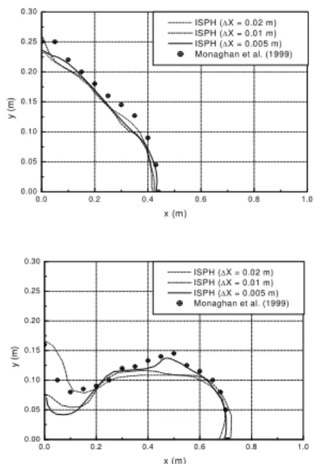
5.3 Convergence Analysis

The computed two-fluid flow interface profiles after the release using three different particle resolutions are compared with the numerical results of

Monaghan et al. (1999), as shown in Fig. 1. The

time sequences of the two figures correspond to t =

1.08 s (upper figure) and 2.155 s (lower figure), respectively.

0.0 0.2 0.4 0.6 0.8 1.0

0.00 0.05 0.10 0.15 0.20 0.25 0.30

ISPH (X = 0.02 m) ISPH (X = 0.01 m) ISPH (X = 0.005 m) Monaghan et al. (1999)

y (

m

)

x (m)

0.0 0.2 0.4 0.6 0.8 1.0

0.00 0.05 0.10 0.15 0.20 0.25 0.30

ISPH (X = 0.02 m) ISPH (X = 0.01 m) ISPH (X = 0.005 m) Monaghan et al. (1999)

y (

m

)

x (m)

Fig. 1. ISPH computed interface flow profiles using different particle resolutions and comparisons with Monaghan et al. (1999).

By comparing the ISPH results with Monaghan et

al. (1999), it is shown that all three ISPH results

agree with Monaghan et al. (1999) reasonably well

for time t = 1.08 s. However, as time goes on to t

can still match the gravity current at the head and the lower body, the gravity current height is significantly underestimated by 25%. In contrast, the most refined ISPH computation matched

Monaghan et al. (1999) quite well and the error is

around 5%. This suggests that the accurate prediction of gravity current height requires much higher particle resolution in the vertical direction, while the gravity current front can be captured with enough accuracy by using a relatively rough particle resolution. It is also observed that there are slightly

large discrepancies near the left wall between x =

0.0 and 0.2 m at time t = 2.155 s. This is due to

some particles are attached to the left wall in both

the present ISPH computations and in Monaghan et

al. (1999). When plotting the free surface, we used

the mean surface levels which resulted in a significant deviation of water surface near the left boundary.

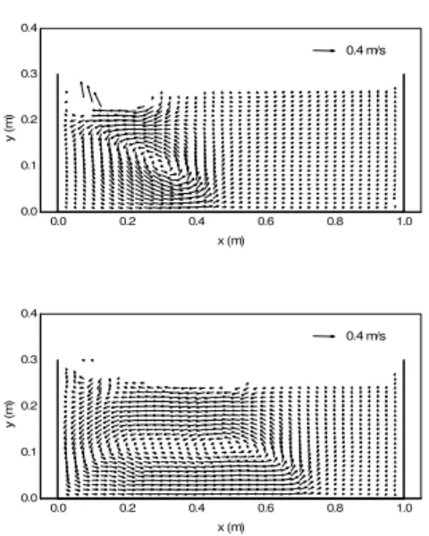
5.4 Sensitivity Study of Spatial Resolutions

The computed flow velocity fields are shown in Figs. 2 (a), (b) and (c), respectively, for the three

different particle resolutions at time t = 1.08 s

(upper figure) and 2.155 s (lower figure). The velocity fields were obtained by mapping the individual particle velocity onto a grid system in the computational domain. The figures showed that all the simulations could equally well disclose the existence of vortexes and circulations formed near the front of the gravity current. However, the most

refined computation by using X = 0.005 m can

predict the velocity structures in a detail manner that both the circulation zone and the constant velocity region of the current head are captured. However, we should note that the velocity fields

computed by X = 0.01 and 0.005 m have a

similar maximum velocity amplitude of 0.4 m/s,

while the coarsest computations by X = 0.02 m

give an unrealistic maximum velocity amplitude of 0.25 m/s, although they have similar velocity structure patterns.

0.0 0.2 0.4 0.6 0.8 1.0

0.0 0.1 0.2 0.3 0.4

0.25 m/s

y (

m

)

x (m)

0.0 0.2 0.4 0.6 0.8 1.0

0.0 0.1 0.2 0.3 0.4

0.25 m/s

y (

m

)

x (m)

Fig. 2. (a) ISPH computed velocity fields by using X = 0.02 m.

0.0 0.2 0.4 0.6 0.8 1.0

0.0 0.1 0.2 0.3 0.4

0.4 m/s

y (

m

)

x (m)

0.0 0.2 0.4 0.6 0.8 1.0

0.0 0.1 0.2 0.3 0.4

0.4 m/s

y (

m

)

x (m)

Fig. 2. (b) ISPH computed velocity fields by using X = 0.01 m.

0.0 0.2 0.4 0.6 0.8 1.0

0.0 0.1 0.2 0.3 0.4

0.4 m/s

y (

m

)

x (m)

0.0 0.2 0.4 0.6 0.8 1.0

0.0 0.1 0.2 0.3 0.4

0.4 m/s

y (

m

)

x (m)

Fig. 2. (c) ISPH computed velocity fields by using

X

 = 0.005 m.

The comparisons in Figs. 1 and 2 suggested that the influence of the spatial resolutions (i.e. particle

spacing X) is relatively small for the macro flow

behaviors, such as the gravity current front propagation, but it could be large for the refined flow structures such as the water splash-up at the free surface and the velocity field. This is due to the fact that some detailed small-scale flows could be lost by using a coarse spatial resolution.

5.5 Pressure and Turbulence Analysis

The computed particle pressure fields are shown in Fig. 3 (a) and (b). In the figures the pressure values have been normalized by the water pressure

per unit depth g and the black lines correspond

between the light and heavy fluids. This indicates that the incompressible pressure solution algorithm of the multi-fluid ISPH model worked well and the interactions between the two fluid components were adequately addressed. Also indicated by the figures is that the pressure integration inside the gravity current is larger than that of the ambient fluid, thus generating enough force momentum for the flow to proceed. Compared with the gravity current profiles (also presented in the figure), it can be found that the pressure contours are nearly equally spaced within both the ambient fluids and the gravity current body. This implies that the pressure distributions in a gravity current flow can be adequately treated as a hydrostatic problem, providing a good rationale that most numerical models based on the SWEs can simulate the gravity current quite well in practice. The latest work of a two-layer SWE

modeling by La Rocca et al. (2012) has supported

such an argument.

-0.2 0.0 0.2 0.4 0.6 0.8 1.0 1.2

0.0 0.1 0.2 0.3 0.4

p/g

(a) t = 1.08 s

y (m

)

x (m)

0 0.05 0.10 0.15 0.20 0.25 0.30 0.35

-0.2 0.0 0.2 0.4 0.6 0.8 1.0 1.2

0.0 0.1 0.2 0.3 0.4

p/g

(b) t = 2.155 s

y (m

)

x (m)

0 0.05 0.10 0.15 0.20 0.25 0.30 0.35

Fig. 3. ISPH computed pressure fields (bold line indicating gravity flow interface profile.

To investigate the turbulence influence during the motion of gravity current, the computed turbulence eddy viscosity distributions are shown in Fig. 4 (a) and (b), and the eddy viscosity values have been normalized by the laminar viscosity of the water. It is found that the maximum eddy viscosity is 50 times higher than the laminar one and this happens at the interface between the heavy and light fluids near the free surface as shown in Fig. 4 (a). Besides, both Fig. 4 (a) and (b) have shown that the larger turbulence areas mainly concentrate near the gravity flow interface. One interesting feature is that the general turbulence eddy viscosity level at the later stage of

the gravity flow at time t = 2.155 s is

approximately half of the early value at time t =

1.08 s. This shows that the flow turbulence tends to affect the early stage gravity flow more.

-0.2 0.0 0.2 0.4 0.6 0.8 1.0 1.2

0.0 0.1 0.2 0.3 0.4

t/0

(a) t = 1.08 s

y (

m

)

x (m)

0 10 20 30 40 50 60

-0.2 0.0 0.2 0.4 0.6 0.8 1.0 1.2

0.0 0.1 0.2 0.3 0.4

t/0

(b) t = 2.155 s

y (

m

)

x (m)

0 5 10 15 20 25 30

Fig. 4. ISPH computed turbulence viscosity fields.

5.6 Sensitivity of Turbulence Modeling on

Flow Profiles

In order to further quantify the influence of turbulence modeling on the gravity flow features, the ISPH model has been re-run without the flow turbulence model. This was realized by deactivating the SPS turbulence model to set the Smagorinsky

constant C_s = 0.0 in the simulations. The computed

particle snapshots are shown in Fig. 5 (a) and (b). Besides, the computed gravity flow profiles in the original run (with the turbulence modeling) are also shown in red lines for a comparison. Comparing the two numerical results, it shows that the computations without the turbulence model produced a stronger water splash near the free

surfaces at the location between x = 0.15 m and 0.2

m at time t = 1.08 s. This is the region where the

heavy fluids collapsed and the returning flow of the light fluids collided with the heavy fluids. In the original ISPH run, the turbulence modeling has dampened the flow energy, leading to a smaller water splash in the free surface. Apart from this, there also exist some minor differences in the interface profile between the two fluid components. In these areas the flow turbulence eddy viscosity assumes relatively larger values so the non-turbulence modeling could induce somewhat different flow features as compared with the turbulence simulations.

6.

MODEL APPLICATION II –

FLOW DOWN A RAMP WITH

THREE FLUIDS

6.1

Engineering Background and Numerical

Settings.

density stratified fluid. The interfaces of the stratified fluids have several effects on the gravity current behaviors, such as diverting the flow direction and initiating the large amplitude wave which has harmful influence over a long distance by changing the flow patterns and dynamics.

According to Yang et al. (2009), the sections of the

offshore slope for most dangerous part of the Jingjiang River with a gradient over 1:2 accounted for 82% in 2006, while it was only 7% in 2002. As a result, the collapse and danger should increase over these slopes and the related sediment pollutant transport studies become more important.

-0.2 0.0 0.2 0.4 0.6 0.8 1.0 1.2

0.0 0.1 0.2 0.3

0.4(a) t = 1.08 s Light particle

Heavy particle

y (m)

x (m)

-0.2 0.0 0.2 0.4 0.6 0.8 1.0 1.2

0.0 0.1 0.2 0.3

0.4 Light particle

Heavy particle (b) t = 2.155 s

y (

m

)

x (m)

Fig. 5. ISPH computed particle snapshots without turbulence modeling (bold line indicating gravity flow interface profile in

original run with turbulence modeling).

To investigate this practical situation, we now consider a steep ramp with 45° slope angle, consisting of a lock fluid region, a horizontal section and a ramp. The lock fluid has a density of

1200 kg/m3 and the lower tank fluid has a density of

1400 kg/m3 overlaid by a fresh water layer with a

density of 1000 kg/m3. According to the numerical

settings of Monaghan et al. (1999), the lock region

has a length 0.5 m and depth 0.25 m. To reduce the computational cost, the left end of tank is set 0.75 m from the bottom of the ramp. The bottom fluid layer has a depth of 0.23 m. The present ISPH computations aim to reproduce the numerical

phenomena of Monaghan et al. (1999) and further

investigate the internal velocity structures during the interaction of three different fluids. A schematic setup of the numerical tank for the ramp flow is shown in Fig. 6. In the selection of model

parameters, an initial particle spacing X = 0.01 m

is used by balancing the computational efficiency and accuracy. There are totally 9041 particles involved, composed of the lock particles, light particles and heavy particles, as shown in Fig. 6. The computation was made by using the AMD Athlon (tm) processor with CPU 1.20 GHz and RAM 256 MB and finished around 20 hours. Different types of the fluid particles were given

different identifiers and thus the free surfaces and interfaces of different fluids can be easily identified in the computations.

-0.8 -0.6 -0.4 -0.2 0.0 0.2 0.4 0.6 0.8 1.0

0.0 0.2 0.4 0.6 0.8

Light particle Heavy partcile Lock particle

y (

m

)

x (m)

Fig. 6. Setup of numerical tank of ramp flow with three different fluids.

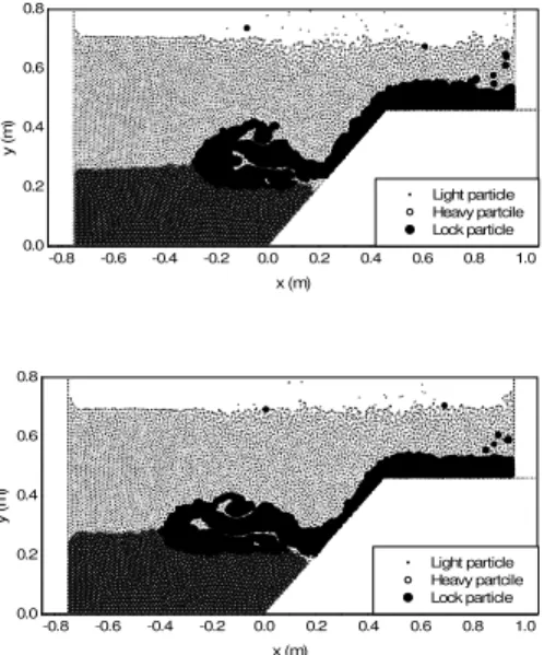
6.2 Computational Results and Analysis

The computed particle snapshots during the flow flowing down a ramp after the release are presented in Fig. 7 at two different times of 3.0 s and 3.4 s (upper and lower figures, respectively), matching

the WCSPH computations of Monaghan et al.

(1999). There is a generally good agreement between the two different SPH modeling

approaches [the results of Monaghan et al. (1999)

are not shown here] and the present model reasonably reproduces the overturning of gravity current head and the subsequent extensive mixing process. From Fig. 7, the ISPH results predict an averaged velocity of the gravity current head of 0.3 m/s, which is within the value range of 0.28 m/s to

0.38 m/s as computed by Monaghan et al. (1999).

Also indicated by our findings, the wave amplitude generated by the descending gravity current in this case is quite small. This is consistent with the

conclusion of Monaghan et al. (1999), which stated

that when the density of the lock fluid is below the density of the bottom layer the wave amplitude is expected to be small.

-0.8 -0.6 -0.4 -0.2 0.0 0.2 0.4 0.6 0.8 1.0

0.0 0.2 0.4 0.6 0.8

Light particle Heavy partcile Lock particle

y (

m

)

x (m)

-0.8 -0.6 -0.4 -0.2 0.0 0.2 0.4 0.6 0.8 1.0

0.0 0.2 0.4 0.6 0.8

Light particle Heavy partcile Lock particle

y (

m

)

x (m)

The computations in Fig. 7 show that when the gravity current descends the ramp and interacts with the interface of the bottom fluid and upper fresh water, it rides over the bottom fluid layer which has a higher density. Due to the relatively steep slope, the vortex motion and flow circulation around the current head are strong and the substantial wrapping and overturning have occurred. The current head is the main site of intensive mixing with the fresh water moving around and behind the head, mixed with the lock fluid. Due to the continuous entrainment of the fresh water with the descending gravity current intruding, the current contains distinct regions of the lower-higher density fluids. There also exist some pockets of the fresh water enclosed inside the lock fluid region.

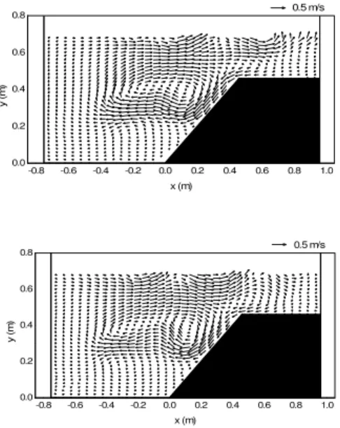
Further examining the velocity fields in Fig. 8, there exist several flow circulation regions. The first figure shows that due to the sudden release of the lock fluid, the gravity current is generated and a counter-current of the fresh water flows into the initial lock region, producing a velocity circulation in the lock region. Besides, stronger flow circulation is found near the current front and a constant velocity region is predicted in the current head. Finally, due to the velocity difference between the lock fluid and the bottom fluid layer, there is a small flow circulation near the interface under the gravity current head, where the amplitude of this flow circulation is quite small, as the density of the lock fluid is smaller than that of the bottom fluid layer. The second velocity figure indicates another very strong flow circulation region just above the ramp slope. Compared with the particle snapshots in Fig. 7, we can observe that this flow circulation is generated due to the lock fluid running down the ramp with high velocity, creating a backwash near the shoreline of the bottom fluid so that the ambient fresh water flows in to compensate for the lock fluid flow. The above particle snapshots and velocity fields have indicated that the gravity current flowing down a ramp has considerable differences in the hydrodynamic concern as compared with a horizontal gravity flow computed in the previous section.

7.

CONCLUSION

To study the Three-Gorges Dam fine sediment pollutant transport, a turbulence multi-fluid ISPH model has been developed to simulate the lock exchange gravity flows generated from the density difference. The model has been applied to the gravity current flowing over a horizontal surface and descending down a ramp to investigate different dam flow effects. The computation results were found in good agreement with the documented data. The computed velocity fields disclosed the distinct flow circulations, and the overturning and wrapping of the fluids have been well captured by the utilized particle modeling approach. The sensitivity tests were also conducted for the proposed numerical model, where the particle resolution was found to be more influential on the refined flow structures such as the free surface breaking, but less on the

macro flow behaviors. The computed pressure fields suggested that the pressure distributions under a gravity flow are essentially hydrostatic and thus the numerical models based on the SWEs should work well for similar applications. The findings of this study should provide necessary considerations for the TGD pollution control unit to minimize the pollutant transport into the downstream of the dam area. However, future work should be carried out to provide more quantitative validations of the model against field data.

-0.8 -0.6 -0.4 -0.2 0.0 0.2 0.4 0.6 0.8 1.0

0.0 0.2 0.4 0.6

0.8 0.5 m/s

y (

m

)

x (m)

-0.8 -0.6 -0.4 -0.2 0.0 0.2 0.4 0.6 0.8 1.0

0.0 0.2 0.4 0.6

0.8 0.5 m/s

y (

m

)

x (m)

Fig. 8. ISPH computed velocity fields of ramp flow with three different fluids.

ACKNOWLEDGEMENTS

The authors acknowledge the support of the Major State Basic Research Development Program (973 program) of China (No. 2013CB036402) and the National Natural Science Foundation of China (No. 51479087).

REFERENCES

Ataie-Ashtiani, B. and G. Shobeyri (2008). Numerical simulation of landslide impulsive waves by incompressible smoothed particle

hydrodynamics. Int. J. Numer. Meth. Fluids 56,

209–232.

Chinese Government State Council (2011). The

State Council Executive Meeting Discusses and Passes the Three Gorges Post-project Plan’. Probe International.

Colagrossi, A. and M. Landrini (2003). Numerical simulation of interfacial flows by smoothed

particle hydrodynamics. J. Comput. Phys. 191,

448–475.

Narayanaswamy (2010). User Guide for the SPHysics Code v2.0.

Gotoh, H. and T. Sakai (2006). Key issues in the particle method for computation of wave

breaking. Coast. Eng. 53, 171–179.

Gotoh, H., T. Shibahara and T. Sakai (2001). Sub-particle-scale turbulence model for the MPS method – Lagrangian flow model for hydraulic

engineering. Comput. Fluid Dyn. J. 9, 339-347.

Guo, G. (2010). Environmental security concerns and the Three Gorges Reservoir Basin in

China. Foundation for Environmental Security

& Sustainability (FESS), Issue Brief 11.

La Rocca, M., C. Adduce, G. Sciortino, A. Bateman Pinzon and M. A. Boniforti (2012). A two-layer, shallow-water model for 3D gravity

currents. J. Hydraul. Res. 50, 208–217.

Monaghan, J. J. (1992). Smoothed Particle

Hydrodynamics. Annu. Rev. Astron. Astrophys.

30, 543–574.

Monaghan, J. J., R. A. F. Cas, A. M. Kos and M. Hallworth (1999). Gravity currents descending

a ramp in a stratified tank. J. Fluid Mech. 379,

39-69.

Monaghan, J. J. and A. Kocharyan (1995). SPH

simulation of multi-phase flow. Comput. Phys.

Commun. 87, 225-235.

Monaghan, J. J., C. A. Meriaux, H. E. Huppert and J. J. Monaghan (2009). High Reynolds number gravity currents along V-shaped valleys.

European Journal of Mechanics B/Fluids 28,

651–659.

Pu, J. H., N. S. Cheng, S. K. Tan and S. D. Shao (2012). Source term treatment of SWEs using

surface gradient upwind method. J. Hydraul.

Res. 50, 145-153.

Rottman, J. W. and J. E. Simpson (1983). Gravity currents produced by instantaneous releases of

a heavy fluid in a rectangular channel. J. Fluid

Mech. 135, 95-110.

Shao, S. D. (2012). Incompressible smoothed particle hydrodynamics simulation of

multifluid flows. Int. J. Numer. Meth. Fluids

69, 1715-1735.

Shao, S. D. (2013). Incompressible SPH simulation of gravity wave generations in a multi-fluid

system. Proceedings of Institution of Civil

Engineers - Engineering and Computational Mechanics 166(EM1), 32-39.

Smagorinsky, J. (1963). General circulation experiments with the primitive equations, I. the

basic experiment. Month. Weather Rev. 91,

99-164.

Subklew, G., J. Ulrich, L. Furst and A. Holtkemeier (2010). Environmental impacts of the Yangtze Three Gorges Project: an overview of the

Chinese-German research cooperation. Journal

of Earth Science 21(6), 817-823.

UC (2012). Summary of Symposium: After 3 Gorges

Dam – What Have We Learned? Department of Landscape Architecture and Environmental Planning, University of California (UC), Berkeley.

Violeau, D. and R. Issa (2007). Numerical modelling of complex turbulent free-surface

flows with the SPH method: an overview. Int.

J. Numer. Meth. Fluids 53, 277–304.

United Nations (2014). Facing the Challenges,

Volume 2. United Nations World Water Development Report

Xu, X., Y. Tan and G. Yang (2013). Environmental impact assessment of the Three Gorges Project

in China. Earth-Science Reviews 124, 115-125.

Yang, G. S., C. D. Ma and E. Y. Chang (2009).