Casson Fluid Flow near the Stagnation Point over a Stretching Sheet with Variable Thickness and Radiation

J_{ournal of} A_pplied F_luid M_{echanics, Vol. 9, No. 3, pp. 1115-1122, 2016.} Available online at www.jafmonline.net, ISSN 1735-3572, EISSN 1735-3645.

Casson Fluid Flow near the Stagnation Point over a

Stretching Sheet with Variable Thickness

and Radiation

G. K. Ramesh

1,2†

, B. C. Prasannakumara

3

,

B. J.Gireesha

2

and M. M. Rashidi

4

1

Department of Mathematics, S.E.A College of Engineering and Technology, K. R. Puram, Bangalore, Karnataka, India

2

Department of Studies in Mathematics, Kuvempu University, Shankaraghatta, Shimoga, Karnataka, India. 3

Department of Mathematics, Government First Grade College, Koppa, Karnataka, India. 4

Mechanical Engineering Department, Engineering Faculty of Bu-Ali Sina University, Hamedan, Iran.

†Corresponding Author Email: gkrmaths@gmail.com

(Received January 22, 2015; accepted June 29, 2015)

A

BSTRACT

The stagnation-point flow of an incompressible non-Newtonian fluid over a non-isothermal stretching sheet is investigated. Mathematical analysis is presented for a Casson fluid by taking into the account of variable thickness and thermal radiation. The coupled partial differential equations governing the flow and heat transfer are transformed into non-linear coupled ordinary differential equations by a similarity transformation. The transformed equations are then solved numerically by Runge-Kutta-Fehlberg method along with

shooting technique. The effects of pertinent parameters such as the Casson fluid parameter, wall thickness

parameter, velocity power index, velocity ratio parameter, Prandtl number and radiation parameter have been discussed. Comparison of the present results with known numerical results is shown and a good agreement is observed.

Keywords: Stagnation point flow; Casson fluid; Variable thickness; Thermal radiation; Numerical solution.

N

OMENCLATURE

A parameter related with sheet profile b parameter related with stretched surfaces

p

c

specific heat

k thermal conductivity

*

k mean absorption co-efficient m velocity power index Nr radiation parameter Pr Prandtl number

r

q radiation heat flux T temperature of the fluid

0

T characteristic temperature w

T temperature at the wall 

T large distance from the wall U free stream velocity

w

U stretching sheet velocity

u_,v velocity components of the fluid along x and y directions

x coordinate along the stretching sheet y distance normal to the stretching sheet  coefficient of viscosity of the fluid  density of the fluid

*

 Stefan-Boltzman constant  similarity variable  stream function  wall thickness parameter  Casson parameter

b

 plastic dynamic viscosity of the non Newtonian fluid

 product of the component of deformation rate with itself

c

 critical value

 ratio of rates of velocities  kinematic viscosity

1.

I

NTRODUCTION

There is an increasing application of non-Newtonian fluids specifically in the flow of nuclear fuel slurries, flow of liquid metal and flow of alloys, flow of plasma, flow of mercury amalgams, and flow of lubrication with heavy oil and greases, coating of papers, polymer extrusion and several others. With such facts in mind, the knowledge of non-Newtonian fluid dynamics with or without heat transfer is quite essential for better understanding regarding food freezing and polymer injection etc. Usually the study of non-Newtonian fluid is much more difficult, because of their complex nature and complex interactions with the flow field. The majority of the information on non-Newtonian fluids is very empirical. The governing equations for non-Newtonian fluid flows are highly nonlinear. Also, the industrial applications of non-Newtonian fluid flow are increasing day by day. Among the many industrial non-Newtonian fluids some fluids behave like elastic solids, and for those fluids, a yield shear stress exists in the constitutive equations. Casson fluid is one of such non-Newtonian fluids. So if the shear stress magnitude is greater than yield shear stress, then flow occurs. Casson model is claimed to fit rheological data better than general viscoplastic models for many materials and is the preferred rheological model for blood and chocolate (1959).Dash et al. (1996) examined Casson fluid flow in a pipe with a homogeneous porous medium. Unsteady boundary layer flow of a Casson fluid due to an impulsively started moving with flat plate has been discussed by Mustafa et al. (2011). Eldabe and Salwa (1995) studied the flow and heat transfer of a Casson fluid between two rotating cylinder. Boyd et al. (2007) analyzed the Casson and Carreau-Yasuda non-Newtonian blood models in steady flow and oscillatory flow using Lattice Boltmann method. Recently Bhattacharyya et al. (2014) obtained the exact solution for boundary layer flow of Casson fluid over a permeable stretching/shrinking sheet. Mukhopadhyay (2013) studied the Casson fluid flow and heat transfer over a nonlinear stretching sheet. At the current investigation, we refer some latest studies on stretched flows. Rashidi and Mohimanian Pour (2010) obtained the analytic solutions for unsteady boundary-layer flow and heat transfer due to a stretching sheet by means of homotopy analysis method. Further Rashidi and Keimanesh (2010) use the differential transform method and Padé approximant for solving MHD flow in a laminar liquid film from a horizontal stretching surface. Rana and Bhargava (2012) studied the flow and heat transfer of a nanofluid over a nonlinearly stretching sheet. Radiation effect on a steady two-dimensional boundary layer flow of a dusty fluid over a stretching sheet is analyzed by Ramesh and Gireesha (2013).

Flow near stagnation-point is very interesting in fluid dynamics. Actually, the stagnation flow takes place whenever the flow impinges to any solid object and the local velocity of the fluid at the stagnation-point is zero. It is an important bearing on several industrial and technical applications such as cooling of electronic devices by fans, cooling of nuclear reactors during emergency shutdown, heat

exchangers placed in a low-velocity environment, solar central receivers exposed to wind currents, and many hydrodynamic processes. The two-dimensional flow of a fluid near a stagnation point was first examined by Hiemenz (1911). Later Chiam (1994) analyzed steady two dimensional stagnation-point flow of an incompressible viscous fluid towards a stretching surface. Mahapatra and Gupta (2002) studied the stagnation-point flow towards a stretching sheet taking different stretching and straining velocities. Various important aspects of the stagnation-point flow over stretching sheet under were presented by many investigators (Nazar et al. 2004, Pal. 2009, Pop et al. 2011, Ramesh et al 2012, Ramesh et al.2014). Mustafa et al. (2012) obtained the analytical solution for stagnation-point flow and heat transfer of a Casson fluid towards a stretching sheet using HAM method. Later Hayat et al. (2013) investigated the mixed convection stagnation-point flow of an incompressible Casson fluid over a stretching sheet under convective boundary conditions. Further Nandy (2013) studied the hydromagnetic boundary layer flow and heat transfer of a non-Newtonian Casson fluid in the neighborhood of a stagnation point over a stretching surface in the presence of velocity and thermal slips. Two-dimensional magnetohydrodynamic stagnation-point flow of electrically conducting non-Newtonian Casson fluid and heat transfer towards a stretching sheet with thermal radiation have been reported by Bhattacharyya (2013). Parand et al (2012) studied the laminar boundary layer flow using numerical method. Akbar et al. (2013) obtained the Numerical solutions of Magnetohydrodynamic boundary layer flow of tangent hyperbolic fluid towards a stretching sheet via RKF45 method.

Aforementioned studies the boundary layer flow and heat transfer analysis is investigated for only flat stretching sheet. Study of flow and heat transfer of viscous fluids over stretching sheet with a variable thickness (non-flatness) can be more relevant to the situation in practical applications. For the first time Fang et al. (2012) obtain an elegant analytical and numerical solution to the two-dimensional boundary layer flow due to a non-flatness stretching sheet. Further this problem was extended by Subhashini et al. (2013) by including the energy equation and found that thermal boundary layer thicknesses for the first solution were thinner than those of the second solution. Numerical solution for the flow of a Newtonian fluid over a stretching sheet with a power law surface velocity, slip velocity and variable thickness was studied by Khaddar et al. (2013).

coefficient and local Nusselt number are tabulated and analyzed. The results have possible technological applications in liquid-based systems involving stretchable materials.

2.

P

ROBLEM

F

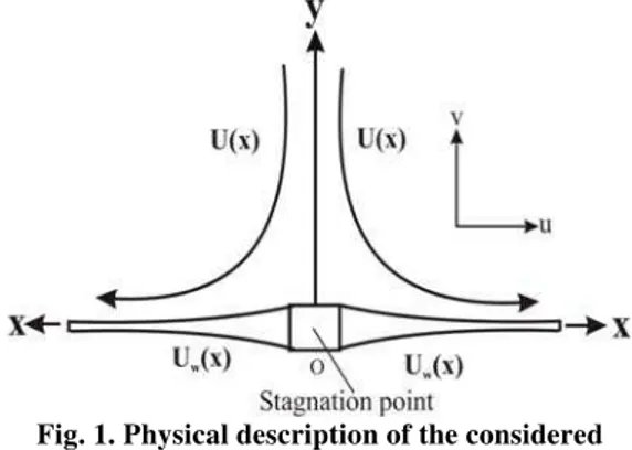
ORMULATION

We consider the steady incompressible flow of Casson fluid over a stretching sheet located at

2 1 ) ( m b x A y  

 with a fixed stagnation point

atx0(figure 1). We assume that wall is impermeable, non-flat with a given profile and the coefficient A being small so that the sheet is sufficiently thin. Assume that the stretching sheet has a velocity U(x)U0(xb)m, where mis the velocity power index.

Fig. 1. Physical description of the considered problem.

The rheological equation of state for an isotropic and incompressible flow of a Casson fluid is









2 / 2 , ,

2 / 2 , .

ij B y ij c

B y c ij c

p e p e              

In above equation  is the product of the component of deformation rate with itself, i.e., e_ije_ij and e_ij is the (i,j)th component of the deformation rate, _c is a critical value of this product based on the non-Newtonian model, _B is plastic dynamic viscosity of the non- Newtonian fluid, and p_y is the yield stress of the fluid.

The simplified two dimensional equations governing the flow in the boundary layer of a steady, laminar, and incompressible Casson fluid are (Bhattacharyya et al. 2014)

0       y v x u

, (1)

x p y u y u v x u u            _        

 1 1 1

2 2

, (2)

y q y T k y T v x T u

c_p r

                 2 2

 , (3)

where uand vare the velocity components of the fluid along x and y directions, respectively,x is distance along the sheet, y is distance perpendicular to the sheet,,,kand

c

_pare the co-efficient of viscosity of the fluid, density of the fluid, thermal conductivity and specific heat of the fluid respectively._B 2_c/p_yis Casson fluid parameter.

The associated boundary conditions for the present problem are [Fang et al. (2012)]

2

0( )

) ( , 0 ), ( m w

w x v T T x T T x b U

u    _  , at

1 2

( ) ,

m

y A x b



 

(4)





U x T T

u ( ), asy,

Where U_w(x)U₀(xb)mis the stretching velocity, U0and b

is uniform velocity of sheet (i.e

for 0m ) and b is a constant. Twand Tdenote the temperature at the wall and at large distance from the wall respectively and T0is the

characteristic temperature

By employing the generalized Bernoulli’s equation, in free stream U(x)U₁(xb)m, equation (2) becomes dx dp dx dU U  1 

 (5)

Using (5) into (2) one can obtain

dx dU U y u y u v x u u          _       2 2 1 1 

 (6)

Using the Rosseland approximation for radiation [19], radiation heat flux is simplified as

y T k q_r     4 * * 3 4

, (7)

Where *and k*are the Stefan-Boltzman constant and mean absorption co-efficient, respectively. Assuming that the temperature differences within the flow such

that the term T4 _{may be expressed as a linear} function of the temperature, we expand T4 _{in a} Taylor series

about T_ and neglecting the higher order terms beyond the first degree in (TT) we get

4 3 4

3

4 _  _

 T T T

T . (8) Using (7) and (8), (3) reduces to

2 2 * 3 * 2 2 3 16 y T k T y T k y T v x T u c_p                   _

The momentum and energy equations can be transformed using the following similarity transformation              A b x y U

m 0 _{( )}m₂1

2 ) 1 (   , 1

0_{( )}

1 2 _    m b x m U f   and     T T T T w w

 , (10)

whereis the similarity variable and is the

stream function defined as y u

 

  and

x v      ,

which identically satisfies equation (1). Substituting (10) into equations (6) and (9), we obtain the following ordinary differential equations:



( )



0

1 2 ) ( ) ( ) ( 1 1 2

2_{  }

           _       f m m f f f

      

(11) 0 ) ( ) ( 1 ) ( ) ( ) ( Pr 1 3 4 1                       f m m f Nr

      

(12)

 

Subjected to the boundary conditions (4) which becomes 0 1 ) ( , 1 ) ( , 1 1 ) (                

 f at

m m f 0 ) ( , ) (    

f as 

(13) In the above equations, prime denote differentiation

with respect to and

  2 ) 1 ( 0 

A U m is the wall

thickness parameter, mis the velocity power index,

0 1

U U



 is the velocity ratio, _*

3 *

4 kk

T

Nr   is the

radiation parameter and k c_p 



Pr is the Prandtl

number.

3.

I

NTRODUCTION OF

R

UNGE

-K

UTTA

-F

EHLBERG METHOD

Runge-Kutta-Fehlberg method has a procedure to determine if the proper step size h is being used. At each step, two different approximations for the solution are made and compared. If the two answers are in close agreement, the approximation is accepted. If the two answers do not agree to a specified accuracy, the step size is reduced. If the answers agree to more significant digits than required, the step size is increased.

Step requires the following values

) 32 9 32 3 , 8 3 ( ) 4 1 , 4 1 ( ) , ( 2 1 3 1 2 1 k k y h x hf k k y h x hf k y x hf k i i i i i i         ) 40 11 4104 1859 2565 3544 2 27 8 , 2 1 ( ) 4104 845 513 3680 8 216 439 , ( ) 2197 7296 2197 7200 2197 1932 , 13 12 ( 5 4 3 2 1 6 4 3 2 1 5 3 2 1 4 k k k k k y h x hf k k k k k y h x hf k k k k y h x hf k i i i i i i                  

An approximation to the solution is madeusing a Runge-Kutta method of order 4:

5 4 3 1 1 5 1 4104 2197 2565 1408 216 25 k k k k y

y_i  _i   

A better value for the solution is determined using Runge-Kutta method of order 5:

6 5 4 3 1 1 55 2 50 9 430 , 56 561 , 28 825 , 12 6656 135 16 k k k k k y z_{i i}

      

4. N

UMERICAL

S

OLUTION

The non-linear coupled equations (11) and (12) along with boundary conditions (13) are solved numerically using Runge-Kutta-Fehlberg method with a shooting technique. In the shooting method, it is essential to select a suitable finite value of

 

 . The step size 0.001issued to obtain the numerical solution with _. The asymptotic converged results within a tolerance level of

6

10 are obtained. Table 1 represents a comparison of f(0)obtained in the present work and those work obtained earlier by Fang et al. (2012) in the absence of ,,Pr,Nr and . It is clearly observed that good agreement between the results exists. This lends confidence in the numerical method. It is also observed from Table 2, that the numerical values of (0)in the present paper for different value of Pr,m are in good agreement with results obtained by Rana and Bhargava (2012) and Zaimi et al. (2014)

5

.

G

RAPHICAL

R

ESULTS AND

D

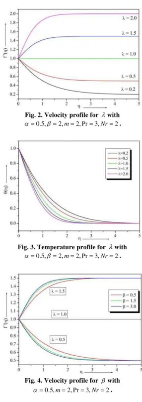
ISCUSSION

represents the velocity and temperature profiles for various values of velocity ratio parameter



.

In figure 2, we can see that two different classes (types) of boundary layers. In the first class, the velocity of fluid inside the boundary layer decreases from the surface towards the edge of the layer (1) and in the second type the fluid velocity increases from the surface towards the edge (1). One important note that if 1, the stretching velocity and the straining velocity are equal, then there is no boundary layer of Casson fluid flow near the sheet, this is similar to that of Chiam’s (1994)  observation for Newtonian fluid. In Fig. 3, one can see that in all cases thermal boundary layers formed and the temperature at a point decreases with increase of.

Table 1 Comparison of the values of skin friction coefficientf(0)for various values ofmin the

case of PrNr0 _and 0.5 m Fang et al. (2012) Present result 10.0 -1.0603 -1.06034

9.0 -1.0589 -1.05893 7.0 -1.0550 -1.05506 5.0 -1.0486 -1.04862 3.0 -1.0359 -1.03588 2.0 -1.0234 -1.02342 1.0 -1.0000 -1.00000 0.5 -0.9799 -0.97994 0.0 -0.9576 -0.95764

Table 2 Comparison of the values of  (0) for various values ofmin the case of

0

    

  Nr N_b N_t



Pr m

Rana and Bhargava (2012)

Zaimi et. al

(2014) Present result

1 0.2 0.6113 0.61131 0.611310 0.5 0.5967 0.5668 0.596687 1.5 0.5768 0.57686 0.576869

2.0 --- 0.57245 0.5724553

3.0 0.5672 0.56719 0.5724553

4.0 --- 0.56415 0.5641562

8.0 --- 0.55897 0.5589740

10.0 0.5578 0.55783 0.5578319

5 0.1 --- 1.61805 1.6180573

0.2 1.591 1.60757 1.6075742

0.3 --- 1.59919 1.5991913

0.5 1.5839 1.58658 1.5865846

0.8 --- 1.57E+00 1.5738902

1.0 --- 1.57E+00 1.5678702

1.5 1.5496 1.55751 1.5575188

2.0 --- 1.55093 1.5509317

2.5 --- 1.54636 1.5463670

3.0 1.5372 1.54271 1.5430156 10.0 1.526 1.52877 1.5287732

Figures 4 and 5 illustrate the influence of the Casson fluid parameter  on the velocity and temperature profiles respectively. One note that the velocity increases with the increase in values of

for (1) and it decreases withfor (1). Consequently, the velocity boundary layer thickness reduces for both values of.The effect of Casson parameter on the temperature profiles is depicted in figure 5 and noticed that at a point temperature increases with increasing of.

Fig. 2. Velocity profile for with

2 , 3 Pr , 2 , 2 , 5 .

0    

  m Nr

 .

Fig. 3. Temperature profile for with

2 , 3 Pr , 2 , 2 , 5 .

0    

  m Nr

 .

Fig. 4. Velocity profile for with

2 , 3 Pr , 2 , 5 .

0   

 m Nr

 .

becomes thicker. The temperature profile for different values of for a fixed value ofis plotted in figure 7. As it can be noticed, an increase in the wall thickness parameter results in an increase of the temperature of fluid.

Fig. 5. Temperature profile for with

2 , 3 Pr , 2 , 5 . 1 , 5 .

0    

  m Nr

 .

Fig. 6. Velocity profile for with

2 , 3 Pr , 2 ,

2   

 m Nr

 .

Fig. 7. Temperature profile for with

2 , 3 Pr , 2 , 5 . 1 ,

2    

  m Nr

 .

Figure 8 shows the effect of on the velocity profiles for the fixed values of other parameters. One can clearly observed that velocity increases with the decrease of and reverse effect can be found when. This indicates that the momentum boundary thickness becomes thinner as increases along the sheet. For a constant valued of temperature increases with the increase of as shown in figure 9. From equation (13), one knows that if the problem reduces to flat sheet problem.

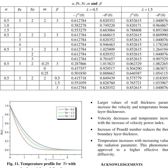
Figure 10 depicts the effect of Prandtl number Pr on temperature distributions for a fixed value of . An increase in Prandtl number reduces the thermal boundary layer thickness. Prandtl number signifies the ratio of momentum diffusivity to thermal diffusivity. Fluids with lower Prandtl number will possess higher thermal conductivities so that heat can diffuse from the wall faster than for higher Pr fluids. Hence Prandtl number can be used to increase the rate of cooling in conducting flows. From figure 11, it is observed that an increase the value of thermal radiation parameter Nr produces a significant increase in the thickness of the thermal boundary layer, so the temperature distribution increases with increasing the value of Nr.

Fig. 8. Velocity profile for mwith

2 , 3 Pr , 5 . 0 ,

2   

  Nr

 .

Fig. 9. Temperature profile for mwith

2 , 3 Pr , 5 . 0 , 5 . 1 ,

2    

   Nr

 .

Fig. 10. Temperature profile for Prwith

2 , 2 , 5 . 0 ,

2   

  m Nr

Table 3 Skin friction coefficientf(0) and Nusselt number  (0)for different values of

m Nr, Pr, ,

 and 

 Pr Nr m  0.5 1.5

) 0 ( f

  (0) f(0)  (0)

0.5 3 2 2 3 0.612784 0.820352 0.852615 1.040076 1.0 0.582278 0.749220 0.820171 0.964867 1.5 0.553279 0.683084 0.788808 0.893380 0.5 2 2 2 3 0.612784 0.668615 0.852615 0.869990

3 0.612784 0.820352 0.852615 1.040076 4 0.612784 0.946463 0.852615 1.178240 0.5 3 1 2 3 0.612784 1.025809 0.852615 1.264194

2 0.612784 0.820352 0.852615 1.040076 3 0.612784 0.701657 0.852615 0.907529

0.5 3 2 -0.25 3 0.287866 1.013823 0.062329 1.082265

0 0.437557 0.929517 0.504290 1.063871

0.25 0.501850 0.888662 0.640387 1.054115

0.5 3 2 2 0.5 0.415718 0.849439 0.575779 1.018303

1.5 0.551059 0.828760 0.765721 1.033967

3 0.612784 0.820352 0.852615 1.040076

Fig. 11. Temperature profile for Nrwith

3 Pr , 2 , 5 . 0 ,

2   

  m

 .

One can note down that momentum equation and heat transfer equation are mutually coupled and the skin friction and Nusselt number coefficient are very important in engineering applications. Therefore the values of f(0)and  (0)are presented in Table 3 for various values of governing parameters at 1and1. It can be seen from the table that the effect of increasing the values ofis to increase the skin friction, whereas



,

m are decreases. Similarly the increasing values of ,Nr,m, is to increase the Nusselt number but the opposite effect can be seen in Pr . Also one can observe that there is no change in the skin friction when Pr and Nr _varies.

6. C

ONCLUSIONS

The main results of present investigation can be listed below.

 Velocity boundary layer thickness decreases with increasing velocity ratio parameter.

 An increase in the Casson parameter decreases the velocity field and increases the temperature field.

 Larger values of wall thickness parameter increase the velocity and temperature boundary layer thicknesses.

 Velocity decreases and temperature increases with the increase of velocity power index.

 Increase of Prandtl number reduces the thermal boundary layer thickness.

 Temperature increases with increasing values of the radiation parameter. This phenomenon is approved to a higher effective thermal diffusivity. 

ACKNOWLEDGEMENTS

The authors are thankful to the referee for his valuable suggestions. One of the author (B. C. Prasanna Kumara) gratefully acknowledges the financial support of University Grants Commission (UGC F. NO. 43-419/2014 (SR)), Delhi, India for pursuing this work.

R

EFERENCES

Akbar, N. S., S. Nadeem, R. U. Haq and Z. H. Khan (2013). Numerical solutions of Magnetohydrodynamic boundary layer flow of tangent hyperbolic fluid towards a stretching sheet. Indian J. Phys. 87(11), 1121–1124.

Bhattacharyya, K. (2013). MHD stagnation-point flow of Casson fluid and heat transfer over a stretching sheet with thermal radiation. J. Thermodynamics 9.

Bhattacharyya, K., T. Hayat and A. Alsaedi (2014). Exact solution for boundary layer flow of Casson fluid over a permeable stretching/shrinking sheet. Z. Angew. Math. Mech. 94(6)522–528.

oscillatory flow using the lattice Boltzmann method. Phys. Fluids. 93-103.

Casson, N. (1959). Rheology of dispersed system, Oxford: Pergamon Press 84.

Chiam, T. C. (1994). Stagnation-point flow towards a stretching plate. J. Phys. Soc. Jpn. 63, 2443– 2444.

Dash, R. K., K. N. Mehta and G. Jayaraman (1996). Casson fluid flow in a pipe filled with a homogeneous porous medium. Int. J. Eng. Sci. 34(10) 1145-1156.

Eldabe, N. T. M. and M. G. E. Salwa (1995). Heat transfer of MHD non-Newtonian Casson fluid flow between two rotating cylinder. J. Phys. Soc.Jpn. 6441–64.

Fang, T., J. I. Zhang and Y. Zhong (2012). Boundary layer flow over a stretching sheet with variable thickness. Applied Mathematics and Computation 218, 7241–7252.

Hayat, T., S. A. Shehzad, A. Alsaedi and M. S. Alhothuali (2012). Mixed Convection Stagnation Point Flow of Casson Fluid with Convective Boundary Conditions. Chin. Phys. Lett. 29(11), 114704.

Hiemenz, K. (1911). Die grenzschicht an einem in dengleich formigen flussigkeitsstrom eingetauchten geraden kreiszlinder. Dingl. Polytec. J. 326, 321–328.

Khader, M. M. and A. M. Megahed (2013). Numerical solution for boundary layer flow due to a nonlinearly stretching sheet with variable thickness and slip velocity. Eur. Phys. J. Plus 128:100 10.1140/epjp/I 2013-13100-7. Mahapatra, T. R. and A. S. Gupta (2002). Heat

transfer in stagnation pint flow towards a stretching sheet. Heat Mass Transf. 38, 517– 521.

Mukhopadhyay, S. (2013). Casson fluid flow and heat transfer over a nonlinearly stretching, Chin. Phys. 22(7), 074701.

Mustafa, M., T. Hayat, I. Pop and A. Aziz (2011). Unsteady boundary layer flow of a Casson fluid due to an impulsively started moving flat plate. Heat Transfer-Asian Resc. 40(6) 563-576.

Mustafa, M., T. Hayat, I. Pop and A. Hendi (2012). Stagnation-point flow and heat transfer of a Casson fluid towards a stretching sheet, Z Naturforsch. 67, 70-76.

Nandy, S. K. (2013). Analytical solution of MHD stagnation-point flow and heat transfer of Casson fluid over a stretching sheet with partial

slip. ISRN Thermodynamics 9.

Nazar, R., N. Amin, D. Filip and I. Pop (2004). Stagnation point flow of a micropolar fluid towards a stretching sheet. Int. J. Nonlinear Mech. 39, 1227–1235.

Pal, D. (2009). Heat and mass transfer in stagnation-point flow towards a stretching surface in the presence ofbuoyancy force and thermal radiation. Meccanica 4, 145–158.

Parand, K., M. Shahini and M. Dehghan (2010). Solution of a laminar boundary layer flow via numerical method. Com. Non. Sci. Num. Sim. 15(2),360-367.

Pop, I., A. Ishak and F. Aman (2011). Radiation effects on the MHD flow near the stagnation point of a stretching sheet: revisited. Z. Angew. Math. Phys. 62(5), 953-956.

Ramesh, G. K. and B. J. Gireesha (2013). Flow over a stretching sheet in a dusty fluid with radiation effect. J heat transfer 135102702(1-6).

Ramesh, G. K., B. J. Gireesha and C. S. Bagewadi (2012). MHD flow of a dusty fluid near the stagnation point over a permeable stretching sheet with non-uniform source/sink. Int. J.Heat and Mass Transf. 55, 4900–4907.

Ramesh, G. K., B. J. Gireesha and C. S. Bagewadi (2014). Stagnation point flow of a MHD dusty fluid towards a stretching sheet with radiation. Afr. Mat. 25(1), 237-249.

Rana, P. and R. Bhargava (2012). Flow and heat transfer of a nanofluid over a nonlinearly stretching sheet: a numerical study. Comm. Nonlinear Sci. Num. Simul. 17, 212-226. Rashidi, M. M. and M. Keimanesh (2010). Using

differential transform method and Padé approximant for solving MHD flow in a laminar liquid film from a horizontal stretching surface. Mathematical Problems in Engineering,. Article ID 491319, 14.

Rashidi, M. M. and S. A. Mohimanian Pour (2010). Analytic approximate solutions for unsteady boundary-layer flow and heat transfer due to a stretching sheet by homotopy analysis method. Nonlinear Analysis: Modelling and Control 15(1), 83–95.

Subhashini, S. V., R. Sumathi and I. Pop (2013). Dual solutions in a thermal diffusive flow over a stretching sheet with variable thickness. Int. Com. Heat and Mass Transf. 48 61–66. Zaimi, K., A. Ishak and I. Pop (2014). Boundary