FORTALEZA
SETEMBRO 2016
Maurício Benegas
Márcio Corrêa
(Un)equal Educational Opportunities
and the Labor Market: A Theoretical
Analysis
SÉRIE ESTUDOS ECONÔMICOS – CAEN Nº 14
(Un)equal Educational Opportunities
and the Labor Market: A Theoretical Analysis
Maurício Benegas Graduate Program in Economics - CAEN/UFC [email protected] Márcio Corrêa Graduate Program in Economics - CAEN/UFC [email protected]
ABSTRACT
This paper studies the effects of public school quality supply on the labor market performance. With this objective in mind, we build a matching model of the labor market with two sectors: schooled and non-schooled. The skilled segment of the economy is endogenous and composed by a continuum of workers who differ in the quality of the school attended. We show that there exists a trade-off between quantity and the quality of education and that a reduction in the schooling costs increases the school enrollment rate. However, it adversely reduces the job creation dynamics in the skilled sector, due to the Composition Effect. We also verify that a first order improvement in school quality distribution may generate an increase in the schooling rate and a greater job vacancy creation in the skilled sector with no negative effects on the unskilled sector.
4 Setembro 2016 INTRODUCTION
1
There are several aspects related to the process of economic and social development. The strong and widespread presence of a traditional and low productive sector, the lack of an appropriate productive infrastructure, low investments in research and development and the misallocation of productive resources, for instance, have all been blamed as the factors behind the strong and persistent process of underdevelopment. The evidence of a large difference in educational achievements between developed and developing economies has led researchers and policymakers to propose investments in public education as one of the main recipes for economic and social development. Focusing on increasing the enrollment rates in primary and secondary education the educational advances in the less developed economies of the world have been striking. In Latin American and Caribbean countries, for instance, the enrollment rates at the secondary education more than double, between 1980 and 2008. The primary completion rate, in turn, reached 100% of the school age population in almost all developing
regions at the same period1.
However, although the school participation rate have improved over the years, international comparisons between the quality of education still reveal strong inequalities between developed and developing countries. In most developing countries, the improvement in completion and school participation rates, for instance, have not been followed by an increases in cognitive tests. The performance gap among students of the same age and year of study has been large and persistent through time.
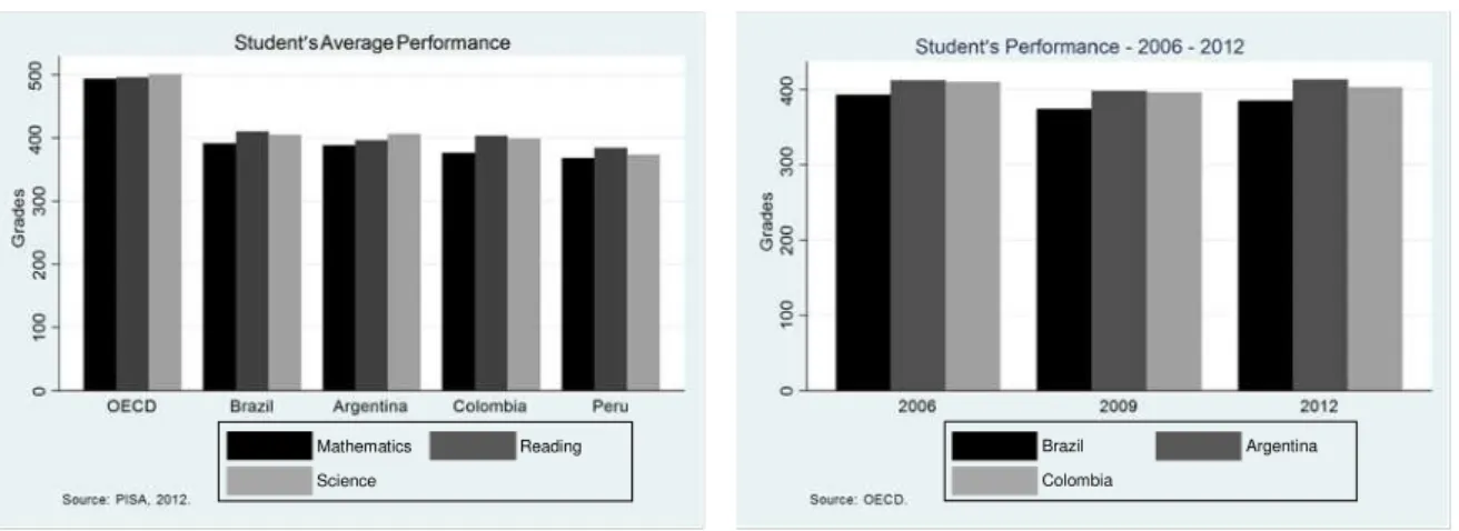
Figures 01 and 02 present the average student’s performance at the OECD countries and some Latin American economies. It can be seen that student’s achievement has not been homogeneous across countries and time. This evidence is even stronger if we
compare the student’sperformance at the richest and the poorest region of the same country. In
Brazil, for example, the average performance of students at the six main metropolitan areas of Brazil - Belo Horizonte, Porto Alegre, Recife, Rio de Janeiro, Salvador and São Paulo - shows that the group enrolled at 9th year of the primary education goes slightly better than their 5th year counterpart. They correctly answered around 60% of the mathematical and reading exams.
The ratio of the top 10% grades to the lower 10% grades also guarantees the evidence of a wide dispersion on the Brazilian student’s performance. The correlation coefficients that follow on Table 1 show the economic and social consequences of having a better school quality. It can be seen that the score obtained by the students of the fifth year is positively related with the completed years of schooling and with the GDP per worker in Brazil.
1 See Glewwe, Hanushek, Humpage, and Ravina (2011) and Prichett (2004) for an overview of the recent public policies and the
5
Brazil Argentina Colombia
Mathematics Reading Science
Figure 01 - Students Performance Figure 02 – Students Performance
The positive impact that education has on the individual development is well known in the economic literature. Card (1999), for example, defended that an additional schooling year implies a growth in the individual wage rate of around 6 to 10%. It has also been defended that human capital investments reduce the incidence of social and health problems and improve a country’s political and financial institutions.
Table 1 - Prova Brasil and SAEB, 2007 - 2013, INEP
5th 9th Total
Mean 196,13 242,32 216,96 Std.Dev. 42,83 44,06 49,09 P10 142,34 182,72 153,39 P90 253,96 301,00 281,07 P90/P10 1,78 1,65 1,83 M aximum 317,17 366,15 366,15
M inimum 94,48 130,43 94,48
Correlation - 5th Grade
Educational Attainment 0,89
GDP per W orker 0,85
Data source: INEP
6 Setembro 2016
the size of the spillover generated by the human capital investments. If the individual returns to education are positive then a policy that induces human capital investments are likely to induce schooling and the aggregate productivity, as proposed by Lucas (1988) and Romer (1990).
The existence of a coordination problem between firms and workers that hampers human capital investments has also been pointed out by the economic literature. According to this view, firms will always invest in the highly skilled sector if there is a sufficient supply of skilled workers in the economy. However, since workers decision to become educated also depend on the labor market expected returns, it is possible to obtain an equilibrium characterized by a poorly skilled sector and a large number of unskilled workers.
Charlot and Decreuse (2005) argued that whenever the link between individual investments in education and the aggregate productivity of the economy is positive, a large amount of individuals will invest in education in order to take advantage of the higher average
productivity of the high educated sector. This effect, known in the literature as Composition
Effect generates a negative impact over the economy. Both the aggregate productivity and the mass of skilled jobs would reduce as the school enrollment rate increases.
The main objective of this paper is the address the link between individual investments in education and the aggregate behavior of the economy. We are particularly interested in evaluate the impact of a policy that increases the school enrollment rate at the labor market and answer the following questions: It is always advantageous to increase the school enrollment rates as we seen in recent years in developing economies? What is the impact of the school quality distribution on the demand of education? What is the link between quantity and quality of education and their effect on the labor market? The unequal provision of public school quality evident in the main developing economies generates negative or positive effects over the labor market?
In order to address the last previous questions and fully internalize the relationship between education and the labor market, we build a dynamic general equilibrium matching model of the labor market based on Pissarides (2000). Our model is composed by a government, that maintains heterogeneous public schools, and a great number of firms and workers that once matched produce a unique consumption good.
The labor market is segmented in the educated and the non-educated sectors. School is voluntary and each individual receives a place to study in a school of
quality q. Then, they must decide between studying and entering the labor force as an unskilled
worker.
The school quality is distributed according to a cumulative distribution function �(�)
with support [�� ,��], where �� and �� are the lowest and the highest quality levels,
7
rate. However, this policy adversely reduces aggregate productivity and the job creation
dynamics in the skilled sector, due to the Composition Effect. We demonstrate that a reduction
in school inequality distribution may generate an increase at the schooling enrollment rate and a greater job creation in the skilled sector with no adverse effects over the unskilled sector of the economy.
To better understand the previous result, consider a Walrasian economy
characterized by a unique level of school quality, �, offered to all individuals in the economy.
Galor and Moav (2004) shown that the size of the educated workforce will be fully characterized by the relative costs and benefits of the human capital investments. Since human capital investments will only be realized if they are properly rewarded, the policy that reduces schooling costs and increases the mass of the educated workers will generate an increase the wage rate
and a positive effects over the aggregate labor market productivity2.
The previous predictions change when there is an imperfect labor market. As
shown by Charlot and Decreuse (2005), the Composition Effect leads to an aggregate
overinvestment in education. In their model with two productive sectors, the schooling costs are proportional to the quality of the school attended. However, as the benefits of education depends on the average quality of the schooled labor force, the relative returns of those that study in low quality schools are higher than the return of individuals that study in better schools. Therefore, the educated workforce tends to be higher than the socially desirable number of individuals.
Our model is characterized by a government that supplies school quality to each agent and the individual productivity is fully described by the quality of the school attended. However, as in Charlot and Decreuse (2005) the marginal benefits of schooling investments are not equal the schooling costs. We show that the stronger the increase in the mass of educated workers, the greater the negative effect of the school enrollment policy over the average quality of the skilled sector.
However, the previous negative effect can be fully eliminated by a different policy that focuses on improving the school quality distribution in the economy. If the benefits of a higher average quality of the schooled labor force are greater than the reduction in the average
quality generated by the Composition Effect, there is a positive effect on the economy.
The present model is related to the growing literature on school quality and returns to schooling investments by Jensen (2004), Eide and Showater (1998), Sauer and Zagler (2014b), Hanushek (2005) and Card and Krueger (1992a). However, the most closely related literature is Charlot and Decreuse (2005) and Charlot, Decreuse, and Granier (2005). All
2 The same previous result can also be found in a more general scenario characterized by a non-degenerate human capital
8 Setembro 2016
models consider the problem of self-selection in education in a friction environment. However, our modeling device differs from these works in some aspects. First, it should be highlighted that all these papers have a completely different focus. We are interested in studying the effects of the school quality distribution on the labor and schooling markets while Charlot and Decreuse (2005) are focused on studying the efficiency of educational choices in a two-sector model. Second, as Kudoh and Sasaki (2002) and Smith (1999), we build a large corporation matching model with heterogeneity in the school quality whilst the previous authors consider a modeling device characterized by one worker and one firm. Finally, unlike the previous authors, we also consider that the skilled segment of the labor market is composed by a continuum of workers who differ in the quality of the school attended. In this way, our model considers that higher schooling quality will result in better worker productivity.
Besides this introduction, this paper has two more sections. In the next section we introduce our benchmark economy and present the main model results. The last section presents the concluding remarks.
THE MODEL 2
The economy is composed by a government, a constant population of individuals and a great number of firms, which once matched with workers, give way to a production of a single consumption good. Firms and workers are risk-neutral and discount the future at the exogenous
and constant rate ρ. Let the time be continuous and consider that each firm has access to a
production technology that exhibits constant returns to scale with labor as the only input.
Companies can be in two different t situations: searching for unemployed workers or producing with all their positions filled. Consider, as Smith (1999) and Cahuc and Wasmer (2001), that the size of the labor force employed by each firm is endogenous. There are two sectors in the labor market, skilled and unskilled, and before opening a vacancy, each company must decide in which sector they will open that position. The public educational system is considered, without loss of generality, to be monopolistic in the production of human capital. Let’s assume it is composed by a continuum of heterogeneous schools with regards to their
quality, �. As in Card and Krueger (1992b), consider that higher school quality results in bigger
return rates on educational investments. Schooling is not compulsory.
9
All infinitely-lived individuals are born with quality �� and they must decide to attend
school for an exogenous fixed period of time �, or to anticipate their entry into the labor force.
Consider that once individuals have decided to study, they receive a take it or leave it vacancy
in a school of quality � and they must pay an exogenous stream of �� units of consumption
good per period as schooling costs, with �> 0.
As Burdett and Smith (2002), consider that agents that decide to study work exclusively in the skilled sector while the group of workers that decide not to attend school work only in the unskilled sector.
The school quality is considered to be fixed over time and we assume, without loss
of generality, that each individual receives only one school offer from the distribution �(�), with
support in the interval [��,�� ]. Consider also that the quality of the school attended is perfectly
observable and it sets the worker’s future productivity in the labor market.
Let Q represent the reservation school quality that makes individuals indifferent
between entering the labor force and studying. Then, it can be shown that agents evaluate working and educational options according to schooling costs and labor market returns from
human capital investments. Whenever � ≥ �, individuals decide to go to school, thus
becoming educated. On the other hand, if � < �, they decide to work in the unskilled sector,
since the labor market returns are bigger than the net benefits received from schooling investments.
Each firm employs skilled and unskilled workers and they optimally decide the number and type of vacancies to open in equilibrium. Suppose as usual in the search literature that, before starting production, workers and firms are involved in a search process to find a
productive partner. Let �� and �� be the search costs of a firm that decides to open a vacancy
in the educated and the non-educated sector, respectively3.
Let �(�/� ≥ �) = ��(�) represent the average quality of the skilled labor force
employed by fi and, as Kudoh and Sasaki (2002) defended, consider that skilled and non-skilled
wage rates are endogenous and given by ��(��) and ��(��), respectively. In turn, consider
that �(����,��(�)��) = [(������+ ����(�)��] represent the production function of a
representative firm matched with �� workers of quality �� and �� workers of average quality
��(�). In this way, we have that each employed worker that studied in a school of quality q
produces ��� units of the consumption good per period, while a worker without studies
produces ���� units of the consumption good, with ���>����,∀� ≥ �.
The number of job matches formed per period is given by a non-negative, concave
and homogeneous degree one matching function, �(��,��), which is crescent in its arguments.
10 Setembro 2016
Let �� represent the vacancy rate and �� denote the fraction of type �= {�,�}
unemployed workers in the economy. By the homogeneity assumption, it can be show that the
probability rate of filling a vacancy is given by: �(��) =�(��,��)
�� , where �� =
��
�� denotes the
tightness of the segment � . In turn, the rate at which an unemployed worker change to
employment status is given by �(��) =���(��) =�(��,��)
�� .
Let �(��) and �(��) be both differentiable in �� and consider that the
unemployment duration rate is limited, for all tightness in the skilled segment of the labor force,
i.e., there is a constant �> 0 such that � 1
�(��)� ≤ � for all �� .
The model is solved recursively. First we focus on the labor market. After typifying the labor market equilibrium we determine individual optimal choice between schooling and early entry into the labor force. The analysis of the education market concludes this section.
2.1. Labor Market
2.1.1 Firms
Let Π(��,��) represent the value function of a firm matched with �� non-educated and ��
educated workers. The following Hamilton-Jacobi-Bellman equation describes the problem of the representative firm:
�Π(��,��) = max
��,��,��,���(1− �)�(����,� �(�)�
�)− ��(��)��− ��(��)��− ����− ����
− �+�Π(��,��)
��� [�(��)��− ����] +
�Π(��,��)
��� [�(��)��− ����]�
(1)
where �(����,��(�)��) = [������+����(�)��]
Equation (1) characterizes the production side of the economy. It tells us that a firm
matched with �� workers of quality �� and �� workers with average quality ��(�) produces
�(����,��(�)��) units of the final consumption good per period.
The firm pays the government as taxes, a fraction � of their final production goods
to finance unemployment benefits and the educational system. The firm also pays ��(��) and
��(��), per period as educated and non-educated workforce rates, respectively. To open an
educated (non-educated) vacancy, the representative company must spend �� (��), as search
11
Let � be an exogenous fixed production cost while the final terms in equation (1) are
related to the flow of non-educated and educated workers between employment and
unemployment statuses. These flows are given by:
�
̇� =�(��)��− ����, where the first elementon the right hand side relates to the rate at which each vacancy becomes occupied. The second term expresses the flow of workers that lose jobs in each period of time.
The set of conditions that characterize the optimal firm decisions are given by4:
��−�Π
(��,��)
��� �
(��) = 0, (2)
��−�Π
(��,��)
��� �
(��) = 0, (3)
��Π(����,��)
� = (1− �)����− ��(��)− �� ′(�
�)��−�Π
(��,��)
��� ��
+�
2Π(� �,��) ���2
[�(��)��− ����] + �
2Π(� �,��)
������ [�(��)��− ����],
(4)
��Π(����,��)
� = (1− �)���
�(�)− �
�(��)− ��′(��)��−�Π
(��,��)
��� ��
+�
2Π(� �,��)
���2 [�(��)��− ����] + � 2Π(�
�,��)
������ [�(��)��− ����].
(5)
Notice that expressions (2) and (3) characterize the optimum supply of vacancy for each type in equilibrium. In turn, equations (4) and (5) determine the size of labor force employed in both sectors. From equations (2) and (3), it can be shown that:
�2Π(� �,��)
���2 = �
2Π(� �,��) ���2
= �
2Π(� �,��) ������ =
�2Π(� �,��)
������ = 0. (6)
By using expressions (2) and (3), together with equation (6), in (4) and (5), we arrive at:
��(�+��)
�(��) = (1− �)����− ��(��)− ��
′(�
�)��, (7)
��(�+��)
�(��) = (1− �)����(�)− ��(��)− ��′(��)��. (8)
12 Setembro 2016
These two previous equations characterize the equilibrium values of �� and ��.
They have a similar interpretation. In this way, let’s focus only on the first equation. The
left-hand side of this expression gives us the expected cost of occupying a type � vacancy. The
other side of the expression is related to the expected profit associated to the creation of a new
vacancy. The equilibrium value of �� is establish in order to equate these two expected returns.
The usual hypothesis of free entry and exit conditions assures us that in equilibrium, all economic rents from opening and closing vacancies are exhausted. Then, we have that:
(1− �)[������+����(�)��] = ��(��)��+��(��)��+������
�(��) +
������
�(��) +� (9)
determines the equilibrium zero profit condition. The left hand side of this expression is related to the firm’s revenues whilst the right hand side gives us the firm costs.
2.1.2 Government
The government raises money to provide unemployment insurance to temporarily unemployed workers and to maintain the public educational system. In this way, let:
�[������+����(�)��] =����+����+�� [1− �(�)]
represents the equilibrium government budget constraint. Again, it can be seen that the left-hand side expresses the government revenue while the right-left-hand side is related to government expenditures.
The amount �� is the marginal cost to finance public education, i.e, �� represents the
additional cost for an additional increment on mass of workers that are studying.
2.1.3 Workers
Let ��(��) and �� (��(��) and ��) be the present worker discounted value of the
expected gains associated to employment and unemployment for an unskilled (skilled) worker.
Notice that an unemployed worker who has studied in a school of quality � receives
13
rate �(��) the educated unemployed worker finds a vacant job, moving to employment status5.
In this way we have that:
���(��) =��(��)− ��(��(��)− ��), (10)
��� =��+�(��)(��(��)− ��), (11)
���(��) =��(��)− ��(��(��)− ��), (12)
���=��+�(��)(��(��)− ��), (13)
determine the value functions of a non-educated and an educated worker, respectively employed and unemployed in the economy. These expressions are standard in search
literature. The first equation implies that a non-educated worker employed in a firm with other ��
unskilled workers receives ��(��) flow units of the consumption good as wages in a given
period. This employed position is destroyed due to an idiosyncratic shock that occurs at rate ��.
Expression (13), in turn, tells us that a worker who studied in his youth receives ��
as unemployment benefits. At rate �(��) this unemployed worker finds a job vacancy moving
into employment status.
If a particular match is destroyed, both the worker and the firm have to pay the costs related to the return to the search process. In this way, a productive match generates a surplus that has to be distributed among the two parties. Consider, as usual in job search theory, that this division is determined by the Generalized Nash Bargain Solution between the firm and the
worker, where �� represents workers bargaining power. The wage rates then satisfy:
���Π
(��,��)
��� = (1− ��)[�� (��)− ��] , (14)
���Π
(��,��)
��� = (1− ��)[�� (��)− ��] , (15)
Observe from these previous expressions that the surpluses generated by the worker and the firm depend on the worker’s quality. If the schooling option is preferred to an
early entry into the labor force, future matching will be of type �. In this case, the wage rate
5 Workers who do not study receive �
� units of the consumption good as an unemployment insurance and they move to an
14 Setembro 2016
must satisfy equation (14). However, if the employee decides to be non-educated, his wage rate must satisfy expression (15).
Using expressions (4) - (6) and (10) - (15), the wage rates are respectively given by:
��=��(1− �)���Γ�+ (1− ��)���� , (16)
��=��(1− �)����Γ�+ (1− ��)��Ψ� , (17)
Where:
Γ� = �
+��+�(��)
�+��+���(��) , (18)
Ψ� = �
+��
�+��+���(��) ,�=�,�. (19)
These two expressions give us the wage rates considering both individuals who
studied and those who didn’t. If � < �, we have agents deciding not to study and the wage
rate once they enter the labor force is given by �� . However, if the school quality satisfies
� ≥ �, we have all individuals going to school and the wage rate is defined by (16).
Notice that the wage rates are a weighted average of two terms: one is related to workers’ job match productivity and the other to the workers’ outside options. Since job match productivity varies if workers attended school or don’t and it is also affected by the quality of the school attended, the first term varies between educated and non-educated workers. Therefore the higher the quality of the attended school, the bigger the job match productivity and the wage rate.
It can also be observed that these two previous expressions are standard in the search literature. However, (16) and its expected counterpart, we described below, deserve some comments:
i) First, it should be noted that it represents the wage rate of an educated worker
who studied in a school of quality �. The expected wage rate is given by:
���=β�(1− �)α���(�)Γ�+ (1− ��)��Ψ�,
where it can be noticed that a higher average productivity ��(�) means a bigger expected wage
15
ii) Let µ represent the mean of the school quality distribution, �(�). It can be shown
that: lim�→����(�) =�� and lim�→����(�) =� 6. These results guarantee that as the size
of the labor force that decides to study goes to the unit, the average productivity converges to
the mean of the distribution of school quality, µ. In turn, as the size of the non-educated labor
force converges to the unit, the average productivity of the educated workforce moves to the
highest value of the distribution, ��.7
iii) The higher the reservation quality � is, the bigger ��� will be8. Notice that a higher
� has two effects over ��: it directly increases the average wage rate of the educated
workforce, due to the higher average productivity of these workers ��(�) , and it indirectly
raises ���, by increasing �
�. In this way, the bigger the size of the labor force that decides not to
study, the higher the wage gap between educated and non-educated workers. It increases ���
by increasing workers’ productivity and their outside option and it does not affect ��.9
iv) Although individuals who decide to study pay the entire cost of schooling, ��, they
receive only part of the return from their investment in education, ��(1− �)���Γ�. This result
gives way to an inefficient amount of school enrolment.10
v) Contrary to SMITH (1999) and CAHUC and WASMER (2001), the wage rate does not depend on the size of the labor force employed by the representative firm This means
that ��(��) =��. This result is a direct consequence of our production function with constant
marginal productivity.11
2.2. Schooling Market and Equilibrium
Once the labor market returns to schooling investment decisions is set, we now define the rule that makes an individual indifferent between investing or not in human capital accumulation.
Let �� be the value function of an unemployed worker with quality ��. Then, we have that:
� �−��� ��� ∞
0 (20)
6 Consider the expression ��(�) = ∫ �
1−�(�)��(�)
��
� . Applying L’Hopital Rule we arrive at these two issues.
7 Consider, for example, that µ < �� . This result can be used to explain the stylized fact that countries with low educational levels
tend to pay higher wage rates to their educated workforce. See Avalos and Savvides (2006), Avalos, Ross, and Sabor (1995), Bils and Klenow (2000) Psacharopoulos and Patrinos (2004) and references therein on this topic.
8 It can be easily show that there is a positive relationship between
� and ��(�). We return to this point later.
9 Goldin (1999) verified this empirical regularity in the United States. 10 This effect is known in literature as
Holdup Problem. See Acemoglu and Shimer (1999) and Acemoglu (1996) among others for
details.
16 Setembro 2016
represents the present value of gains related to an early entry into the labor force.
However, if someone decides to study, the expected discounted present valued of such decision would be given by:
� �� −�� −����� 0
+� �−������
∞
� ∕ � ≥ ��
, (21)
where the first term is associated to the schooling costs materialized during the compulsory
period �. The following term refers to the benefits of being an educated worker with quality
� ∈ [�,�� ].
Assumption 1: The schooling costs must satisfy the restriction:
ρ(���−1) �< β�(1− �)α��(��)
��+��+���(��)� .
This prior hypothesis is needed to guarantee that there are always educated and non-educated workers in the economy. Otherwise, workers would never invest in schooling
since the benefits to become educated would not compensate for related costs.12
From expressions (20) and (21) we have that whenever individuals decide to study.
� �� −�� −������ 0
+� �−������
∞
� ∕ � ≥ �� ≥
� �−������
∞
0
, (22)
The following proposition establishes the equilibrium value of �.
Proposition 1: The schooling reservation quality that leaves individuals indifferent between
study and work activities �, satisfies:
��(�) =��(��)− �(��)
�(��) � (23)
where,
12 We could alternatively establish this assumption in terms of the maximum schooling period. In this particular case, it is necessary
17
�(��) =����(1− �)α����(��)��+ (�+��)��
�+��+���(��) � ,
�(��) = (�+��)��
�+��+���(��) ,
�(��) =(1− �)α����(��)[�+��+���(��)]��
��(1− �−��)�
�+��+���(��) .
Proof: See Appendix I
The previous proposition establishes the minimum public school quality compatible with the indifference between studying and working options. If the school quality offered to an
individual is defined in [�,�� ], he/she will always study, becoming a skilled worker after �
periods. However, if the school quality offered to this particular worker is in [��,�), he/she will
never study.
Definition:A steady-state equilibrium for this economy is an eleven-tuple:
(��,��,��,��,��,�)such that �� = ��
�� and �(��)��=���� , for �= {�,�} , and equations (7), (8), (9),
(16), (17), (23) and the government budget constraint are satisfied.
The equilibrium has a block recursive structure. Using expressions (17) and (7) we
obtain the equilibrium values of ��,�� . It can be seen that the equation that characterizes the
equilibrium value of �� does not depend on �� and �. By using a similar reasoning, equations
(16) and (8) determine the equilibrium value of
�
�� and �� . They are both functions of �. Theexpressions that characterize the equilibrium values of �� and ��(�) are given by:
(��− ��)
�(��) =
(1− ��)[(1− �)����− ��]
�+��+���(��) , (24)
(��− ��)
����(�)�
=(1− ��)[(1− �)���
�(�)− � �]
18 Setembro 2016
Notice that if the equilibrium value of � exists, it can be determined by replacing ��(�) in (25)13.
The following theorem shows that the equilibrium exists.
Theorem 2: Consider that if the school quality offered to an individual is given by � = ��,
he/she never studies. If, additionally
���(�+��)��+��(1− �)�����(��∗)
�+��+���(��∗) − ���� <
(�+��)��+��(1− �)��������(��)�
�+��+������(��)� − �
����� �,
then there is at least one� ∈(��,��)that satisfies expression (25)
Proof: See Appendix II
The previous theorem uses two conditions that deserve further comments. Suppose that an unskilled worker changes his/her mind and decides to be educated after receiving a
school offer of quality �� . The last condition establishes that evaluated on �, the net payoff of
such decision will always be lower than the payoff received if the student decided to become skilled in the beginning of his life. In our opinion, this hypothesis seems reasonable and corroborates the widely accepted stylized fact in human capital investment literature that
individuals invest in schooling in earlier stages of life and in training activities in future periods.14
The other condition that guarantees the equilibrium existence comes from the fact
that whenever the school quality is given by ��, individuals will always decide not to study. This
hypothesis seems also reasonable because no workers would like to pay for an investment that offers no net returns.
Finally, it should also be noticed from the previous theorem that the differentiability
of ��(�) is a sufficient condition for equilibrium unicity. In fact, using the Implicit Function
Theorem in the skilled job creation condition, it can be shown that �� and � are directly
related. Therefore, if ��′(�) exists, it is strictly positive, implying that �(�) is strictly decreasing.
In turn, ��(�) is differentiable if �′(�� ) and �′(��) do not vanish in equilibrium.
Proposition 3:Consider the steady state equilibrium. An increase in � and � imply an increase
in �� and � and no effect over �� .
Proof: See Appendix III
13 Notice that
��(�)is the solution of the previous expression (23).
19
The last proposition shows the impact of an increase in � and � on the labor and the
educational markets. First, it can be seen that an increase in the schooling period or the schooling cost have no effect on the job creation dynamics in the unskilled sector. However, they have a positive impact on the high-quality sector job creation flows and a negative impact
on the schooling rate, through their positive effect over �.
The positive impact of a lower schooling rate on the skilled sector is known as the
Composition Effect. The reason of this impact is due to the effect that a higher schooling cost exerts in the economy. Notice that the higher the incentive to become non-educated, the bigger
will be the average productivity of the educated workforce ��(�). This new value of �, in turn,
implies that the average productivity of the educated workers increases. Then, although the
schooling rate might be decreasing with a higher value of �, the average productivity increases,
encouraging the creation of new jobs in high-quality sector15
It can also be observed from the last proposition that a higher schooling period or a bigger schooling cost will mean a better job composition. However, the negative aspect of this
last policy is that it attracts a higher wage gap between educated and non-educated workers.16
Definition: Let �(�), defined in the support [��,�� ] be the distribution of the public education
quality (���). We say that the government provides a first-order improvement in ��� if there is
a new distribution �(�) such that: �(�) ≿ ���� �(�).17
Proposition 4: Let µ� = ��[�] and µ� = �� [�] be the expected values of � under distributions �(�) and � (�). Also consider that the respective conditional expected values are given by: ���(�) =�
�[� �⁄ >�] and ��� (�) = �� [�/� > �]. A First-Order Improvement in PEQ reduces
the equilibrium value of �. Furthermore,
i) If �� <���(��∗) then exists a unique � ∈(��,��∗] such that ������=���(��∗).
Moreover, if
a) ��∗ <�, then � � �(�
�∗) <���(��∗);
b) ��∗ ≥ �, then �
� �(�
�∗)≥ ���(��∗).
ii) If �� ≥ ���(�
�∗), then ���(��)≥ ���(��∗) for any � ∈[��,��]. Proof: See Appendix IV
15 See also Charlot and Decreuse (2005) and Charlot and Decreuse (2005) and references there in on the impact of the
Composition Effect over the incentives to become educated. Rosenzweig and Evenson (1977) and Rosenzweig (1990) stated that
low schooling enrollment in developing economies is the result of high schooling costs. See also Rammohan (2000) on the effects of high schooling costs on child labor enrollment and Ravalion and Wodon (2000) on the connections among schooling costs and school attendance versus child leisure.
16 In a study on the effects of mass school construction in Indonesia, Duflo (2001) verified the existence of a negative relationship
between schooling costs and school enrollment. Pischke and von Wachter (2008) concluded that an increase in the schooling period in Germany generated no impacts in the wage rate.
20 Setembro 2016
The previous proposition shows that, if �(�) and � (�) are the distribution functions
before and after a school quality improvement policy, then we must have as a result that ��<∗ ��∗.
In other words, the first-order improvement in school quality distribution turns the workers
decision to become educated a more attractive option, reducing the equilibrium value of �.
However; this last proposition also leads us to conclude that although there is an increase in
schooling enrollment, the impact of a first-order improvement in school quality over ��(�) and ��is
not certain.
To see this result, consider that if the reduction in � comes with a higher value of
��(�), the previous policy generates a higher job creation dynamics in the skilled sector. This
will happen, for example, if the new unconditional average school quality is higher than old conditional average quality. If this is the case, a better quality school distribution policy shall cause a higher aggregate schooling rate and a bigger job creation dynamics in the educated
sector. However, if this is not the case, the result of a higher � is a reduction in ��(�),.
CONCLUDING REMARKS 3
The main objective of this paper is to evaluate the impact of the public school quality provision on the labor and education market equilibrium. We built a matching model in the spirit of Pissarides (2000) increased with endogenous human capital schooling investments and free fi entry in the skilled and unskilled sector. In our model, workers human capital is a positive function of the quality of the school attended during their student days. The paper shows, for instance, that a first-order improvement in the school quality distribution generate an increase in the aggregate schooling rate and a higher job creation dynamics in the skilled sector. We also showed that this policy generates an increase in the skilled sector size. However, it also implies a higher wage inequality between the skilled and the unskilled sector. We also evaluate the impact of higher schooling costs on the school enrollment rate and the labor market performance.
References
Acemoglu, D. (1996): “A Microfoundation for Social Increasing Returns in Human Capital Accumulation”, The Quarterly Journal of Economics, 111(3), 779–804.
Acemoglu, D., and R. Shimer (1999): “Holdups and Efficiency with Search Frictions”, International Economic Review, 40(4), 827–849.
21
Avalos, N., D. Ross, and R. Sabor (1995): “Inequality and Growth Reconsidered: Lessons from East Asia”, The World Bank Economic Review, 9(3), 477–508.
Becker, G. (1962): “Investment in Human capital: A Theoretical Analysis,” Journal of Political Economy, 70(5), 9–49.
Billingsley, P. (1986): Probability and Measure. Willey and Sons, New York
Bils, M., and P. Klenow (2000): “Does Schooling Cause Growth?”, American Economic Review, 90(5), 1160–1183.
Burdett, K., and E. Smith (2002): “The Low Skill Trap”, European Economic Review, 46(8), 1439–1541.
Cahuc, P., F. Marque, and E. Wasmer (2008): “A Theory of Wage and Labor Demand with Intra-Firm Bargaining and Matching Frictions”, International Economic Review, 49(3), 943–972.
Cahuc, P., and E. Wasmer (2001): “Does Intrafirm Bargaining Matter in the Large Firm’s Model?”, Macroeconomic Dynamics, 5(5), 742–747.
Card, D. (1999): Causal Effect of Education on Earnings. Amsterdan: North Holland.
Card, D., and A. Krueger (1992a): “Does School Quality Matter? Returns to Education and the Characteristics of Public Schools in the United States”, Journal of Political Economy, 100(1), 1–40.
______. (1992b): “Does School Quality Matter? Returns to Education and the Characteristics of Public Schools in the United States”, Journal of Political Economy, 100(1), 1–40.
Charlot, O., and B. Decreuse (2005): “Self Selection in Education with Matching Frictions”, Labour Economics, 12(2), 251–267.
Charlot, O., B. Decreuse, and P. Granier (2005): “Adaptability, Productivity, and Educational Incentives in a Matching Model”, European Economic Review, 49(4), 1007–1032.
Duflo, E. (2001): “Schooling and Labor Market Consequences of School Construction in Indonesia: Evidence from an Unusual Policy Experiment”, American Economic Review, 91(4), 795–813.
Eide, E., and M. Showater (1998): “The Effect of School Quality on Student Performance: A Quantile Regression Approach”, Economics Letters, 58(3), 345– 350.
Galor, O., and O. Moav (2004): “From Physical to Human Capital Accumulation: Inequality and the Process of Development”, Review of Economic Studies, 71, 1001– 1026.
Glewwe, P., E. Hanushek, S. Humpage, and R. Ravina (2011): “School Resources and Educational Outcomes in Developing Countries: A Review of the Literature from 1990 to 2010”, NBER, Working Paper 17554.
Goldin, C. (1999): “Egalitarianism and the Returns to Education during the Great Transformation of American Education”, Journal of Political Economy, 107(6), 65–94.
22 Setembro 2016
Jensen, R. (2004): “The (Perceived) Returns to Education and the Demand for Schooling”, Quarterly Journal of Economics, 125(2), 515–548.
Kudoh, N., and M. Sasaki (2002): “Employment and Hours of Work”, European Economic Review, 55(2), 176–192.
Lucas, R. (1988): “On the Mechanics of Economic Development”, Journal of Monetary Economics, 22(1), 3–42.
Pischke, J. S., and T. von Wachter (2008): “Zero Returns to Compulsory Schooling in Germany: Evidence and Interpretation”, The Review of Economics and Statistics, 90(3), 592–598.
Pissarides, C. (2000): Equilibrium Unemployment Theory. Oxford: Basil Blackwell.
Prichett, L. (2004): “Access to Education”, Global Crises, Global Solutions.
Psacharopoulos, G., and H. Patrinos (2004): “Returns to Investment in Education: A Further Update”, Education Economics, 12(2), 111–134.
Rammohan, A. (2000): “The Interaction of Child Labor and Schooling in Developing Countries: A Theoretical Perspective”, Journal of Economic Development, 25(2), 85–99.
Ravalion, M., and Q. Wodon (2000): “Does Child Labor Displace Schooling?”, Economic Journal, 110(2), 158–175.
Romer, P. (1990): “Endogenous Technological Change”, Journal of Political Economy, 85(5), 71–102.
Rosenzweig, M. (1990): “Population Growth and Human Capital Investments: Theory and Evidence”, Journal of Political Economy, 98(5), 38–70.
Rosenzweig, M., and R. Evenson (1977): “Fertility, Schooling, and the Economic Contribution of Children of Rural India: An Econometric Analysis”, Econometrica, 45(5), 1065–79.
Sauer, P., and M. Zagler (2012): “Economic Growth and the Quantity and Distribution of Education: A Survey”, Journal of Economic Surveys, 26(5), 933–951.
______. (2014a): “(In) equality in Education and Economic Development”, Review of Income and Wealth, 60(November).
______. (2014b): “(In) equality in Education and Economic Development”, The Review of Economic and Wealth, 60(11), 353–379
23 Appendix I
Proof of Proposition 1
We know that ��(�) =∫ �
1−�(�) ��
� ��(�). Then, we have that:
��� �� =
�(�)
1− �(�)[��(�)− �] > 0
Now, let the distribution of school quality with compact support [��, ��] be absolutely
continuous with a finite first moment. Then we can rewrite expression (23) as:
� �−���
�(��)��=− ∞
0 � �
−����(� � ≥ �⁄ )�� �
0
+� �−���(��(�)
∞
� ∕ � ≥ �
)��,
for all � ∈(��,��]. Since �(� �⁄ ≥ �) =��(�), we have that:
(I)
� �−��[�
�(��) +���(�)]��= �
0 � �
−���[�
�(�)− ��(��)]�� ∞
0
,
for all � ∈(��,��]. Using (17) - (20) in (11) - (14) we arrive at:
��(�) =
(�+��)��+ (1− �)�����(��)��(�)
�[�+��+���(��)] ,
��(��) =
(�+��)��+ (1− �)�����(��)��
�[�+��+���(��)] ,
Finally, considering these two last expressions in (I) we obtain the equilibrium value of ��(�).
24 Setembro 2016 Appendix II
Proof of Theorem 2
Lemma 5: Under the assumption that � 1
�(��)� ≤ �, for all ��, the vacancy duration rate is Lipschitz with constant �, where�=��� � �
�(��)� 1 �(��)��.
Proof: Notice that
� �(��)�
1 �(��)�=
�′(��) �(��)2 .
Considering �(��) as the skilled sector job creation elasticity, we have that
� �(��)�
1 �(��)�=
�(��) �(��) .
Since �(��)∈(0,1), we have that
� �(��)�
1
�(��)�<�
i.e. vacancy duration rate has limited derivative. We then conclude that 1
�(��) is Lipschitz with
constant�, where�=��� � �
�(��)� 1 �(��)��.
Lemma 6: Let ��(�) be the solution of (25). Then, ��(�) is continuous in �.
Proof: Rearranging expression (25), together with the equality �(��) =���(��), we arrive at
(1− ��)[(1− �)����(�)− ��] =��(�+��)
����(�)�+������(�) .
Let �(�) = (1− ��)[(1− �)����(�)− ��]. From the Martingale Convergence Theorem, we
know that �(?) is continuous for all �18
25
In this way, we have that
������(�) =�����(�+��(��)�) .
For � fixed, let �> 0 arbitrary. Then, there is a �> 0 such that
����|��(�)− ��(�)| <� − ��(�+��)�����1(�)�− 1 ����(�)�� ,
for all � ∈ ��(�). By using Lemma 5, the previous inequality implies that
����|��(�)− ��(�)| <� − ��(�+��)� |��(�)− ��(�)| ,
or
��|��(�)− ��(�)| <�′ ,
where �′= �
(��−��)[��+(�+��)�]> 0.
Now, we can write expression (24) as
(II)
���(�+��)��
�+��+������∗�+
�����(1−�)�����(� �∗)
�+��+������∗� −
(�+��)��
�+��+������(�)�− �
��(1−�)������(�)�
�+��+������(�)� − �(�
��−1)�� ��(�) = 0 .
To proceed in the demonstration we need to show that ����(�)� is continuous in �. Now, since
26 Setembro 2016 Proof of Theorem 2: Rewrite (II) as:
�(�) = �
��(�+� �)�� �+��+���(��∗)+
����
�(1− �)�����(��∗) �+��+���(��∗) −
(�+��)��
�+��+������(�)�
− ���(1− �)������(�)� �+��+������(�)�− �(�
��−1)�� ��(�) .
The reader can easily verify that the condition
���(�+��)��+��(1− �)�����(��∗)
�+��+���(��∗) − ����<
(�+��)��+��(1− �)��������(��)�
�+��+������(��)� − �
����� � ,
together with the fact that every individual does not study if the school quality received is given
by �=��, is insufficient to guarantee that:
(III)
�(��) < 0 <�(��).
Therefore, the continuity of �(�) and the fact that ��∈(��,��) such that:
27 Appendix III
Proof of Proposition 3
Consider again that ���(��) =�(��), for �= {�,�}. Rewrite (24) to (25) as:
� (��,��,�) � =� �(�)− ��(��)− �(��) �(��) �, � (��) � = �+��+���(��) �(��) −
(1− ��)[(1− �)����− ��]
(��− ��) ,
� (��,�)
� =
�+��+���(��)
�(��) −
(1− ��)[(1− �)����(�)− ��]
(��− ��) ,
where �(��),�(��) and �(��) are given by the previous expressions in the text.
Notice that:
� =−�
���
��′(��)(�+��)[(1− �)����− ��]
[�+��+���(��)]2 < 0;
′
���
=���
′(�
�)(�+��)[(1− �)����(�)− ��]
[�+��+���(��)]2 ;
� ={(1− �)�����(��)−[�+��+���(��)]��
��(1− �−��)�}�′�(�)
[�+��+���(��)]2 > 0;
′
�,�
� = ���
′(�
�)�(��)− �′(��)[�+��+���(��)]
[�+ (��)]2 > 0; =� = 0
′
�,�� ′
�,��
; � = 0;
′
�,�
�′ = 0
�,��
; � = ���
′(�
�)�(��)− �′(��)[�+��+���(��)]
[�+ (��)]2 > 0
′
�,��
;
� =− (1− ��)(1− �)���
′�(�)
��− �� < 0
′
�,�
.
28 Setembro 2016
�′ =−����(1− �−��)��(�) < 0;
�,�
� = 0;
′
�,� �
= 0;
′
�,�
� = 0;
′
�,� �
= 0;
′
�,�
Since the determinant of the principal matrix – the matrix with the derivatives of
∑�, ∑� and ∑� with respect to �,�� and �� is non-singular, we can show by the implicit
function theorem that:
���
�� = 0;
��� �� > 0;
�� ��> 0;
���
�� = 0;
��� �� > 0;
29 Appendix IV
Proof of Proposition 4
Lemma 7: Let �′(� �⁄ ) =�[� �⁄ >�] and ��′(� �⁄ ) =�[� �⁄ >�], for all �>�. If
�(�)≻���� �(�), we have that: �′(� �⁄ )≻���� �′(� �⁄ ), for every � ∈[��,��], we have that
�′(� �⁄ ) >�′(� �⁄ ). Now, by definition we have that:
�(�)− �(�) 1− �(�) >
�(�)− �(�) 1− �(�) ,
which can be written as:
�1− �(�)� � ��(�) >�1− �(�)�
��
� � ��
(�) ,
��
�
or after some calculation as:
�1− �(�)� � ���(�)− �(�)�
��
�
>��(�)− �(�)� � ��(�) .
��
�
This last inequality implies that:
�(�)− �(�)≤0 ,
for some �. This result is the opposite of �(�)≻���� �(�).
Proof of Proposition 4: Consider assumption 1. Then,
��(1− �)���(��)
�+��+���(��)− �(���−1)�> 0
assures that
�(�) =� −���
�
0 ����
+� �−����(�)�� .
∞
30 Setembro 2016
Is increasing in �. From Lemma 7 we have that:
��[�(�)⁄�>�]≥ ��[�(�)⁄�>�] .
But, from worker decisions we know that:
��[�(�)⁄�>�]≥ ��[�(�)⁄�>��∗] =� �−����(��)�� . ∞
0
where ��∗ is the optimal decision with distribution �(�). Therefore, whenever:
��[�(�)⁄�>��∗] =� �−����(��)�� , ∞
0
we have ��∗ ≤ �
�∗. Now, let
ℎ(�) =���(�)− ���(��∗) .
This previous inequality, together with the continuity of ℎ(. ), imply that there exists a
�� ∈(��,��∗] such that ℎ(��) = 0 . Since the function ���(. ) Is increasing, we have that:
��∗ <�� ⟹ ���(��∗) <���(��) =���(��∗) ;
��∗ ≥ �� ⟹ ���(��∗)≥ ���(��) =���(��∗) ;
The unicity of �� is guaranteed by the monotonicity of ���(. ).
Finally, it is necessary to remember that ���(�)≥ �
� �(�
�) =��, for any value of � ∈[��,��], to
Av. da Universidade, 2700 Benfica Fone/Fax:(085) 3366.7751 Cep: 60.020-181 Fortaleza - CE - Brasil