Outcome Prediction in Mathematical Models
of Immune Response to Infection
Manuel Mai1*, Kun Wang2,3, Greg Huber4, Michael Kirby2,5, Mark D. Shattuck3,6, Corey S. O’Hern1,3,7,8
1Department of Physics, Yale University, New Haven, Connecticut, United States of America,2Department of Mathematics, Colorado State University, Fort Collins, Colorado, United States of America,3Department of Mechanical Engineering and Material Science, Yale University, New Haven, Connecticut, United States of America,4Kavli Institute for Theoretical Physics, Kohn Hall, University of California Santa Barbara, Santa Barbara, California, United States of America,5Department of Computer Science, Colorado State University, Fort Collins, Colorado, United States of America,6Benjamin Levich Institute and Physics Department, The City College of New York, New York, New York, United States of America,7Department of Applied Physics, Yale University, New Haven, Connecticut, United States of America,8Graduate Program in Computational Biology and Bioinformatics, Yale University, New Haven, Connecticut, United States of America
Abstract
Clinicians need to predict patient outcomes with high accuracy as early as possible after disease inception. In this manuscript, we show that patient-to-patient variability sets a fun-damental limit on outcome prediction accuracy for a general class of mathematical models for the immune response to infection. However, accuracy can be increased at the expense of delayed prognosis. We investigate several systems of ordinary differential equations (ODEs) that model the host immune response to a pathogen load. Advantages of systems of ODEs for investigating the immune response to infection include the ability to collect data on large numbers of‘virtual patients’, each with a given set of model parameters, and obtain many time points during the course of the infection. We implement patient-to-patient vari-abilityvin the ODE models by randomly selecting the model parameters from distributions with coefficients of variationvthat are centered on physiological values. We use logistic regression with one-versus-all classification to predict the discrete steady-state outcomes of the system. We find that the prediction algorithm achieves near 100% accuracy forv= 0, and the accuracy decreases with increasingvfor all ODE models studied. The fact that mul-tiple steady-state outcomes can be obtained for a given initial condition,i.e.the basins of attraction overlap in the space of initial conditions, limits the prediction accuracy forv>0. Increasing the elapsed time of the variables used to train and test the classifier, increases the prediction accuracy, while adding explicit external noise to the ODE models decreases the prediction accuracy. Our results quantify the competition between early prognosis and high prediction accuracy that is frequently encountered by clinicians.
a11111
OPEN ACCESS
Citation:Mai M, Wang K, Huber G, Kirby M, Shattuck MD, O’Hern CS (2015) Outcome Prediction in Mathematical Models of Immune Response to Infection. PLoS ONE 10(8): e0135861. doi:10.1371/ journal.pone.0135861
Editor:Andrew J. Yates, University of Glasgow, UNITED KINGDOM
Received:March 30, 2015
Accepted:July 27, 2015
Published:August 19, 2015
Copyright:© 2015 Mai et al. This is an open access article distributed under the terms of theCreative Commons Attribution License, which permits unrestricted use, distribution, and reproduction in any medium, provided the original author and source are credited.
Data Availability Statement:All relevant data are within the paper.
Introduction
The immune response to infection is a complex process that involves a wide range of length scales from proteins to cells [1–4], tissues [5], and organ systems [6]. Despite enormous prog-ress over the past 30 years in developing mathematical models for the immune response to infectious disease such as tuberculosis [7,8], HIV [9–13], and influenza [14,15], these models still have not been able to dramatically improve patient diagnosis, prognosis, and treatment [16,17]. Instead, vaccine and drug development often relies on costly trial-and-error methods [18]. However, advances in gene sequencing capabilities [19], increasing speeds of computer processors, and the ability to store enormous amounts of medical data promise dramatic improvements in mathematical approaches to predicting and controlling the response to infec-tious disease [20–23].
One promising mathematical approach is to use machine learning methods on large data sets to classify patients as healthy or sick, perform early warning analyses for early detection of infection, or identify the minimal set of genes responsible for a particular immune response. [24,25] However, many questions are left unanswered in such studies. For example, how much and what kinds of data are required to have confidence in the machine learning predictions and what are the underlying biophysical mechanisms for the relationships between variables that are identified by these techniques? Further, it is difficult to determine differences in the immune response that arise from patient-to-patient variations compared to slight differences in the initial conditions of each patient.
In this manuscript, we focus on sets of ordinary differential equations (ODEs) as mathemat-ical models for the immune response to infection. The advantages of ODEs are manifold: 1) Each‘virtual patient’can be considered as a set of parameters in the set of ODEs; 2) There is essentially no limit on the amount of data that can be collected on each virtual patient; 3) The accuracy of machine learning predictions can be explicitly tested as a function of the number of time points and initial conditions for each patient and the number of patients included in the training and testing sets; and 4) analysis of the fixed points (or steady-state outcomes) and basins of attraction of the ODEs can give biophysical insight into the immune response to infection.
We will investigate several classes of ODE models for the immune response to infection. First, we will describe a four-dimensional model for the acute inflammatory response to a path-ogen load that was studied in detail in Ref. [26]. We will then consider reduced versions of this model with fewer variables and parameters obtained by slaving one or more of the original four variables, as well as changes to the form of the ODEs that alter the fixed point structure and flows between them. For each model, a virtual patient is defined by one set of parameters. Given an initial condition (values of the variables at timet= 0), the patient will evolve deter-ministically to one of several possible discrete steady-state (t! 1) outcomes, or fixed points. Thus, for each patient, we can determine the basins of attraction that map initial conditions for all of the variables to steady-state outcomes by numerically integrating the sets of ODEs.
We seek to determine the limits of the prediction accuracy of discrete steady-state outcomes of ODEs as a function of patient variability (i.e.random fluctuations in parameter values) using machine learning techniques. In the limit of zero patient variability, our simple classifica-tion algorithm (logistic regression) can achieve nearly perfect predicclassifica-tion accuracy even when the classification occurs on variables at short times. However, as the patient variability increases, the basins of attraction for different patients yield different outcomes for a given ini-tial condition as shown inFig 1for 5% patient variability in model (1) for the immune response to infection. (SeeMaterials and Methods). The fact that each set of initial conditions does not possess a unique outcome places a fundamental limit on the predictability of patient outcomes.
(K.W. and M.K.). This work also benefited from the facilities and staff of the Yale University Faculty of Arts and Sciences High Performance Computing Center and NSF Grant No. CNS-0821132 that partially funded acquisition of the computational facilities. The funders had no role in study design, data collection and analysis, decision to publish, or preparation of the manuscript.
Thus, we find that the machine learning prediction accuracy decreases with increasing patient variability. In contrast, for a given patient variability, the prediction accuracy increases with the time used for classification as the systems converge to their steady-state outcomes (Fig 1). We also show that at short times our classification algorithm saturates the theoretical limit for the prediction accuracy in the presence of patient variation, and that the addition of external noise only worsens the outcome prediction accuracy.
The manuscript is organized as follows. In the Materials and Methods section, we introduce several ODE systems that have been used to model the host immune response to infection [26], including their parameter sets and discrete steady-state outcomes, and describe how we imple-ment patient variability in the ODE models. We also describe the logistic regression classifica-tion algorithm that we implement to predict steady-state outcomes and measures of the performance of the classification algorithm. In the Results section, we emphasize our three main results that hold for all of the ODE models we studied: 1) patient variability leads to over-lap of the basins of attraction for the steady-state outcomes, which limits the outcome predic-tion accuracy, 2) the predicpredic-tion accuracy increases with the time used for classificapredic-tion because the basins of attraction separate with increasing time, and 3) the addition of external measure-ment noise further reduces the prediction accuracy. In the Discussion section, we point out the clinical implications of our work and describe important future studies of the prediction accu-racy for ODE models with continuous, rather than discrete, steady-state outcomes.
Materials and Methods
Our studies focus on several ODE models with varying complexity for the immune response to pathogen load that were first introduced in Ref. [26]. These ODE models can have up to four coupled variables that represent the concentration of pathogenP, activated neutrophilsN, inflammation (or damage)D, and immuno-suppressor (cortisol)C. The models include inter-actions between these four quanties. For example, the presence of pathogenP>0 causes an immune response, where neutrophils are activated andNincreases. Neutrophils kill pathogen, which decreasesP, but also cause inflammation (damage), which increasesD. The cortisol level
Cincreases when there is a high neutrophil level, which then reduces the neutrophil level. Model (1) (Eqs1–4) includes all four variablesP,N,D, andC. The right-hand side ofdP/dt
is a sum of three terms. The first term enables logistic growth of the pathogen. In the absence of any other terms, any positive initialP0will causePto grow logistically to the steady-state valueP1. The second term mimics a local, non-specific response to an infection. For small
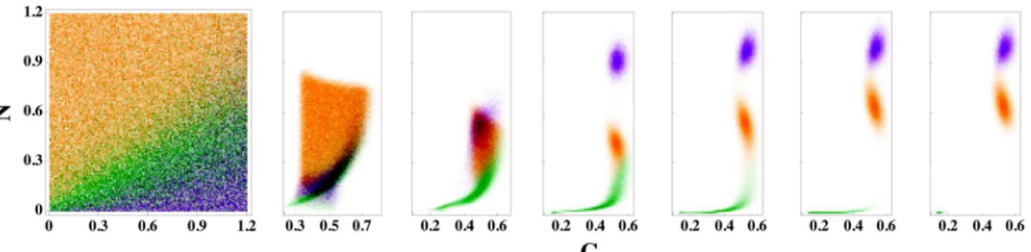
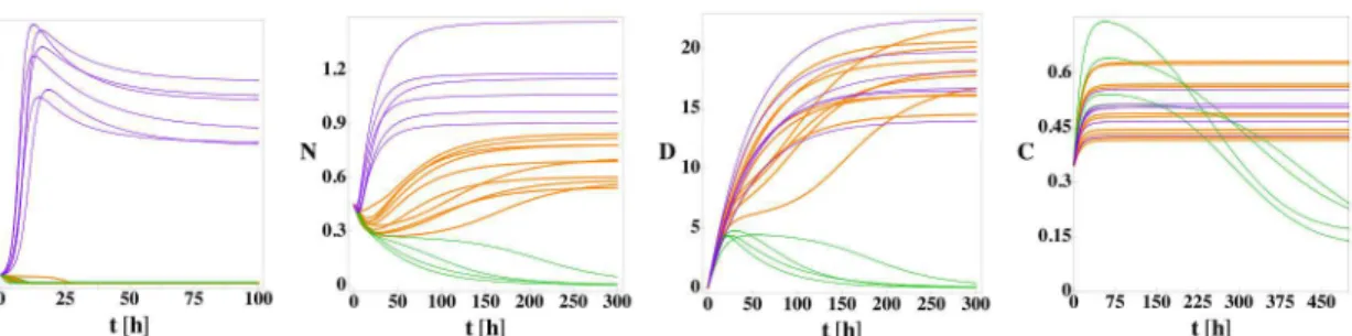
Fig 1. Time evolution of patient outcomes for a range of neutrophil (N) and cortisol (C) initial conditions for model (1).(left) Patient outcomes in the long-time limit givenNandCinitial conditions for model (1) are shaded green, orange, and purple for the steady-state outcomes of health, aseptic, and septic death, respectively. The initial values of the pathogen load and damage areP0= 0.35 andD0= 0, and patient variability is set tov= 5%. The right six panels indicate how the systems in the leftmost panel separate in theNandCplane as time increases,t= 10, 20, 50, 100, 250, and 500, from left to right.
values ofP, the decrease is proportional toP. For larger values ofP, the decrease caused by the second term is constant. The third term models the decrease ofPdue to interactions with acti-vated immune cells (neutrophils)N. Activated neutrophilsNcan directly decreaseP. The anti-inflammatory response, which is captured by the cortisol levelC, mitigates this effect leading to a decrease ofPproportional toNP/(1 + (C/C
1)2).
Two terms determine the rate of change in neutrophils,dN/dt. The first term accounts for the fact that neutrophils can be activated if a resting neutrophil cell encounters a pathogenPor an already activated neutrophilN. Furthermore, tissue damageDalso triggers the activation of neutrophils. The second term describes the death of neutrophilsN, with the decrease inN pro-portional to the amount of neutrophils present.
The rate of change in damagedD/dtis also controlled by two terms. The first term mimics positive feedback betweenDandN. Activated phagocytes cause collateral damage in the tissue. Again, the effectiveness ofNis mitigated by the anti-inflammatory response 1/(1 + (C/C1)2). The saturation functionfsmodels the fact that the effect ofNonDsaturates for largeN. The second term, -μdD, represents repair of the tissue.
The anti-inflammatory responseCincreases with the source termsc. In addition, there is a natural death rateμc, which leads to a positive steady-state value ofCin the absence of any immune activationNor damageD. However, even small amounts of damage and neutrophils will up-regulateC. In the case of smallN+kcndD, the production ofCis proportional toN+
kcndD, while for large values ofN+kcndD, changes inCare proportional tokcn. Again, the effectiveness ofNis mitigated by 1/(1 + (C/C1)2).
Model (1) has 21 parameters:kpm,kmp,sm,μm,kpg,P1,kpn,knp,knn,snr,μnr,μn,knd,kdn,xdn,
μd,C1,sc,kcn,kcnd, andμcwith units provided inTable 1. Depending on the values of these parameters, model (1) possesses different numbers of fixed points with varying stabilities. However, we will focus on a specific parameter regime (given inTable 1) with three stable fixed points, which correspond to the physiological steady-state outcomes: health, septic death, and aseptic death.
Model (1)
dP
dt ¼ kpgP 1
P P1
k
pmsmP
mmþkmpP
kpnfðN;CÞP ð1Þ
dN dt ¼
snrR
mnrþR mnN ð2Þ
dD
dt ¼ kdnfsðf Nð ;CÞÞ mdD ð3Þ
dC dt ¼ scþ
kcnfðNþkcndD;CÞ
1þfðNþk
cndD;CÞ
mcC; ð4Þ
where
R¼fðknnNþknpPþkndD;CÞ; ð5Þ
fðV;CÞ ¼V=ð1þ ðC=C 1Þ
2
Þ; ð6Þ
fsðVÞ ¼V
6 =ðx6
ndþV
6
Models (2)-(5) given below are simplified versions of model (1). A summary of the dimen-sion, number of parameters, and number of stable fixed points for each of these ODE models is shown inTable 2. To obtain model (2) from (1),Cis set to a constantC¼0:23and the
remaining terms define a three-variable model withP,N, andD. For model (3), we setC¼C
andD= 0, which gives a two-variable model forPandN. For model (4), we setC¼Cand P= 0 to obtain a two-variable model forNandD. In this model, the value of the initial rise in
Ncan be thought of as the response to trauma. For model (5), we setC¼C¼0:1,D= 0, and N= 0, which gives a one-dimensional model forP. This model only treats the innate immune response with no activated neutrophils.
Model (2)
dP
dt ¼ kpgP 1 P P1
k
pmsmP
mmþkmpP
kpnfðN;CÞP ð8Þ
dN dt ¼
snrR
mnrþR mnN ð9Þ
dD
dt ¼ kdnfs f N;
C
ð Þ
ð Þ mdD ð10Þ
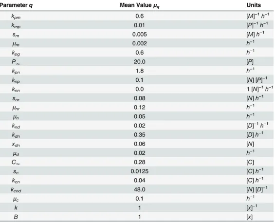
Table 1. Mean values and units for the ODE parameters.The mean valuesμqand their units for the the
twenty-three parametersqfor models (1)-(6). [y] indicates the dimension ofyand time is measured in hours (h).
Parameterq Mean Valueμq Units
kpm 0.6 [M]−1h−1
kmp 0.01 [P]−1h−1
sm 0.005 [M]h−1
μm 0.002 h−1
kpg 0.6 h−1
P1 20.0 [P]
kpn 1.8 h−1
knp 0.1 [N] [P]−1
knn 0.0 1 [N]−1h−1
snr 0.08 [N]h−1
μnr 0.12 h−1
μn 0.05 h−1
knd 0.02 [D]−1h−1
kdn 0.35 [D]h−1
xdn 0.06 [N]
μd 0.02 h−1
C1 0.28 [C]
sc 0.0125 [C]h−1
kcn 0.04 [C]h−1
kcnd 48.0 [N] [D]−1
μc 0.1 h−1
k 1 [x]−1
B 1 [x]
Model (3)
dP
dt ¼ kpgP 1 P P1
k
pmsmP
mmþkmpP
kpnfðN;
CÞP ð11Þ
dN dt ¼
snrR3
mnrþR3
mnN; ð12Þ
where
R3¼fðknnNþknpP;
CÞ: ð13Þ
Model (4)
dN dt ¼
snrR4
mnrþR4
mnN ð14Þ
dD
dt ¼ kdnfs f N;
C
ð Þ
ð Þ mdD; ð15Þ
where
R4¼fðknnNþkndD;
CÞ: ð16Þ
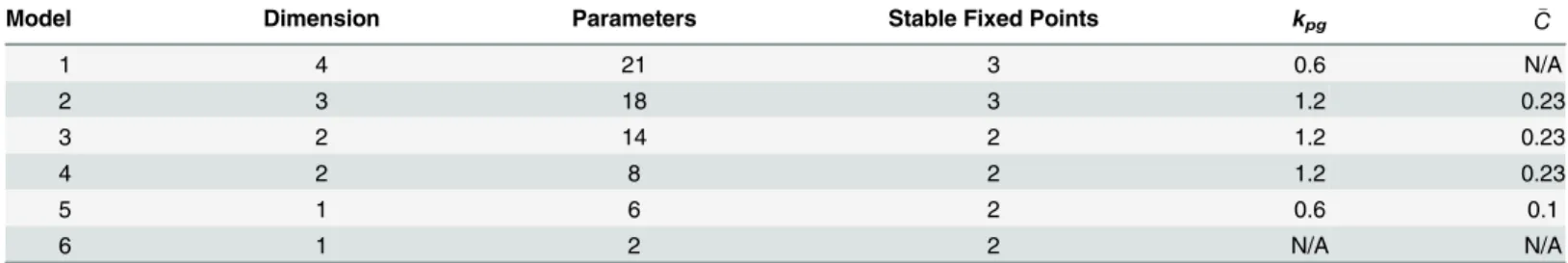
Table 2. Summary of the ODE models.The dimension, number of parameters, number of stable fixed points, and values for the key parameterskpgandC
for models (1)-(6).
Model Dimension Parameters Stable Fixed Points kpg C
1 4 21 3 0.6 N/A
2 3 18 3 1.2 0.23
3 2 14 2 1.2 0.23
4 2 8 2 1.2 0.23
5 1 6 2 0.6 0.1
6 1 2 2 N/A N/A
doi:10.1371/journal.pone.0135861.t002
Fig 2.P,N,D, andCversus time for model (1) from 20 random initial conditions with no patient variation.For the parameter values inTable 1but with
kpg= 1.2, model (1) possesses three fixed points: health (green lines), septic death (purple lines), and aseptic death (orange lines). The initial conditions are
sampled randomly within the cube: 0P00.42, 0N00.255,D0= 0, and 0C00.35. The three fixed points can be differentiated by the steady-state values ofPandD: health (P= 0,D= 0), aseptic death (P= 0,D>0), and septic death (P>0,D>0). 5, 13, and 2 of the initial conditions evolve to the health,
septic death, and aseptic death fixed points, respectively.
Model (5)
dP
dt ¼kpgP 1
P P1
k
pmsmP
mmþkmpP
ð17Þ
InFig 2, we show the time evolution of the four variablesP,N,D, andCfor model (1) for twenty different sets of random initial conditions to illustrate its three stable fixed points (health, septic death, and aseptic death) using the parameter values inTable 1. For trajectories that approach the septic death fixed point, the pathogen and neutrophil levels grow rapidly. The high neutrophil level causes cortisol to increase as well. Despite the high level, the neutro-phils cannot reduce the pathogen load and the cortisol level is not large enough to reduce the neutrophil level. As a result, the high neutrophil level causes significant damage at long times, which is termed septic death due to the associated high pathogen level. Thus, the septic death steady-state outcome is characterized byP>0,N>0,D>0, andC>C1.
In the healthy state, the pathogen level can be reduced to zero by the neutrophils, and the neutrophil level can be reduced to zero by cortisol. Once the neutrophil level is zero, the corti-sol level returns to its background level and damage decreases to zero. Thus, the healthy state is characterized byP= 0,N= 0,D= 0, andC=C1.
During the approach to the aseptic death fixed point, the neutrophil level is strong enough to reduce the pathogen level to zero, but the cortisol level is insufficient to reduce the neutro-phil level to zero, which leads to increasing damage. Thus, the aseptic death fixed point is char-acterized byP= 0,N>0,D>0, andC>C1.
We also studied a generalization of model (5). Model (6) is a one-dimensional ODE for the variablexwith the same fixed point structure as model (5) (Eq 17), but different locations for the fixed points, which can be obtained by tuning the two parameterskandB.
Model (6)
dx=dt¼ Bcosðk xþp=
2Þ; if 0x2p=k
B ksinð5p=2Þðx 2p=kÞ; if 2p=k<x: ð18Þ
(
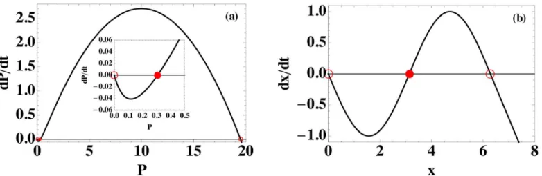
Model (5), which is a one-dimensional ODE for pathogenP, possesses threefixed points:P= 0, 0.3078, and 19.49 for the mean parameters inTable 1. As shown inFig 3(a), the two outerfixed
Fig 3. Comparison of ODE models (5) and (6).The functionsf(P) =dP/dtandf(x) =dx/dtfor models (a) (5) and (b) (6). (See Eqs(17)and(18)). Stable and unstable fixed points are marked by open and filled circles, respectively. Both models share the same fixed point topology: one stable fixed point at zero and one at a positive value. The unstable fixed point lies between the two stable fixed points. The inset in (a) magnifiesdP/dtnear the origin.
points for model (5) are stable, and the middlefixed point, which is near zero, is unstable. For model (6), the central unstablefixed point is moved to the midpoint of the two outer stable fixed points and the shape of the function is changed to retain thefixed point structure.
Fig 4summarizes the interactions between all of the variables in models (1)—(6). Green, solid arrows connecting pairs of variables indicate upregulation, while red, dashed bars indicate downregulation. For all models, both up and down self-regulation can also occur. If the sign of the feedback (i.e.positive or negative) depends on the values of the variables and parameters, self-regulation is represented using both an arrow and bar beginning and ending on a single variable.
The outcomes of the immune response to infection can vary from patient to patient, even with the same initial conditions (e.g.the pathogen load) (SeeFig 5). To introduce patient vari-ability into the ODE models, we select the parameters ({q}) in models (1)-(6) randomly from independent Gaussian distributions with mean valuesμqinTable 1and standard deviation
Fig 4. Interactions between variables for models (1)—(6).The green, solid arrows betwen pairs of variables denote upregulation and the red, dashed bars indicate downregulation for ODE models (1)-(6). Combined dashed and solid arrows indicate that either up or downregulation is possible depending on the values of the variables and parameters.
doi:10.1371/journal.pone.0135861.g004
Fig 5.P,N,D, andCversus time for model (1) with 20 sets of randomly selected parameters with the same initial conditions.10% patient variation allows the system to reach the health, aseptic, and septic death fixed points with the initial conditionP0= 0.45,N0= 0.45,D0= 0, andC0= 0.35, whereas only the septic death fixed point is obtained for this initial condition with no patient variation. 4, 6, and 10 of the trajectories evolve to the health, septic death, and aseptic death fixed points, respectively. The means of the parameters were set to those provided inTable 1, except the mean ofkpg= 0.8 was chosen to
display maximum variability of the steady-state outcomes.
relative to the mean (or coefficient of variation)v. Negative values of the parameters can cause the ODE models to become non-integrable, and thus the parameter distributions are cut off so that the parameter values are non-negative. (We also studied log-normal distributions for the parameters, which ensure thatq>0, and found qualitatively similar results). We solve the ODE models (1)-(6) for 104sets of parameters for each of the 104random initial conditions at eachv. The limits for the sampling of the initial conditions for each model are given inTable 3. We then perform classification analyses on these trajectories to predict the steady-state outcomes.
The prediction accuracyAis defined as the number of correct classifications of the steady-state outcomes divided by the total number of classifications. The accuracy quantifies the qual-ity of the prediction of all of the steady-state outcomes and is therefore a discriminating mea-sure of the overall performance of the classifier. We also evaluated the performance of the classifier separately for each of the predicted steady-state outcomes. For model (1), there are three steady-state outcomes, and thus there are three possible true-positive rates (TPR), one for each outcome. In addition, there are two false-negative rates (FNR) for each outcome. Com-plete quantification of the performance can be obtained using the 3 × 3 confusion matrix of the classifier. There are several combinations of entries of the confusion matrix that can be plotted against each other. In the Results section, we plot the TPR versus the FNR values as well as the accuracy to assess the performance of the classification analyses.
We employ logistic regression to obtain predictions for the steady-state outcomes. A logistic regression algorithm, in its most basic form, is a method to classify data into two groups. Based on input dataxðiÞ¼ ðxðiÞ
1 ;x
ðiÞ
2 ;. . .;x
ðiÞ
NÞ, we attempt to predict the class labely(i)2{0, 1} (i.e.
steady-state outcome). In our case, the input data are the model variables at a specified timetc, whereNis the number of variables in the model. To train the classifier, we employ labeled training data (x(i),y(i)). The logistic regression algorithm thenfits a logistic function
PyðxðiÞÞ ¼ 1
1þey0þy1x1iþy2xi2þþyNx
i N
ð19Þ
to the training data. The parametersθj, wherej= 0, 1, 2,. . .,N, are determined by minimizing the cost function
Jðy0;y1;. . .;yNÞ ¼
1
m
Xm
i¼1
yðiÞlogðPyðxðiÞÞÞ þ ð1 yðiÞÞlogð1 P
yðx
ðiÞÞÞ
" #
; ð20Þ
wheremis the number of training samples. EvaluatingPθ(x(k)) on an unseen data pointx(k)
gives the probability thaty(k)= 1. IfPθ(x(k)) is greater than some threshold 0<c<1, we predict
the label to bey(k)= 1, otherwisey(k)= 0. A typical value for the threshold isc= 1/2, but it can
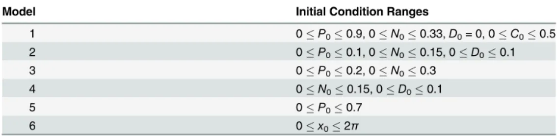
Table 3. Summary of the initial condition ranges used in the ODE models.The ranges of the initial condi-tions for each of the variables in ODE models (1)-(6).
Model Initial Condition Ranges
1 0P00.9, 0N00.33,D0= 0, 0C00.5
2 0P00.1, 0N00.15, 0D00.1
3 0P00.2, 0N00.3
4 0N00.15, 0D00.1
5 0P00.7
6 0x02π
be tuned to increase either the precision or the recall of the classifier. Thefitting process identi-fies the parametersθjsuch that the classification error on the training set is minimal.
Models (1) and (2) possess three steady-state outcomes (aseptic death, septic death, and health), therefore we must go beyond the binary classification scheme described above. To clas-sify ODE models with three steady-state outcomes, we implement the one-versus-all classifica-tion scheme. To do this, we consider three outcome labels,yðhiÞ,y
ðiÞ
ad, andy
ðiÞ
sd, for a given set of
variablesx(i).yhðiÞ¼0if the patient outcome is not health (i.e.aseptic or septic death) andy
ðiÞ
h ¼
1if the patient outcome is health. Similar definitions apply foryðiÞ
adandy
ðiÞ
sd (SeeTable 4). We
use these outcome labels andEq 20to determine three probability functions,Ph(x),Pad(x), and
Psd(x). Given an unlabeled set of variablesxðkÞ ¼ ðx1ðkÞ;x
ðkÞ
2 ;. . .;x
ðkÞ
N Þ, we calculatePh(x(k)),
Pad(x(k)), andPsd(x(k)) and select the outcome with highest probability to be the predicted outcome.
Results
For a deterministic system of ODEs, the basin of attraction for a given fixed point is defined as the collection of initial conditions that evolve to that particular fixed point. For a given set of parameters, each of the ODE models (1)-(6) possesses well-defined (non-overlapping) basins of attraction for each fixed point.
However, different outcomes can be achieved even for a single initial condition if the param-eters of the ODE model are varied. (SeeFig 5). For example, the ratio of the parametersscand
μcdetermines the background level of cortisol in model (1). Background cortisol levels are known to vary from patient to patient and can vary from one organ system to another in a given patient. To mimic these variations, we select sets of parameters randomly with mean val-ues inTable 1and standard deviations relative to their mean values (i.e.coefficient of variation) given byv. (SeeMaterials and Methods). With patient variation, an initial condition can pos-sess multiple outcomes, and thus the basins of attraction for the fixed points overlap as shown inFig 1.
We seek to predict the patient steady-state outcomes in models (1)-(6) in the presence of patient variabilityv. For the prediction method, we employ logistic regression with one-versus-all classification [27]. (SeeMaterials and Methods). We compare the prediction accuracyAat patient variabilityvto the average best guess of the steady-state outcome. For the best guess method, we determine the steady-state outcome for each of 102sets of parameters for a given initial condition. We define the best guess as the steady-state outcome with the highest number of occurrences and record the frequencyfiof the best guess for initial conditioni. We then average the frequencyfiover 103initial conditions for eachvto obtain an estimate for the pre-diction accuracy in systems with basin overlap.
For the prediction method, we solve a given system of ODEs forNi= 104random initial conditions, each with randomly selected parameter sets with coefficient of variationv. We chooseNt= 800 of theNitrajectories randomly to train the classifier and predict the outcome of the remaining 9200 trajectories. The classifier maps the state of the system at a given timetc
Table 4. One-versus-all classification of outcomes.The three one-versus-all classifications for ODE mod-els with three steady-state outcomes.
Class 1 (y= 0) Class 2 (y= 1)
septic death + health aseptic death
health + aseptic death septic death
aseptic death + septic death health
to a particular steady-state outcome. The prediction accuracy is then averaged over 10 training and prediction runs, each withNt= 800 randomly selected training trajectories.
InFig 6, we compare the accuracyAof the logistic regression prediction method (with clas-sification at timetc= 0) to the average best-guess frequency as a function of the patient variabil-ityvfor models (1)-(5). For all model ODEs, the prediction accuracy for the logistic regression prediction method is near 100% atv= 0, decreases for increasing patient variability, and reaches a plateau near 1/nfin the largevlimit, wherenfis the number of stable fixed points in the model (except for model (3)). For model (3) with two steady-state outcomes, the prediction accuracy is non-monotonic and increases forv>0.3 because this ODE model begins to sample parameter regimes where one steady-state outcome is much more probable than the other. In addition, for all models the average best-guess frequency provides an upper bound for the accu-racy of the prediction algorithm. Hence, the overlap of the basins of attraction imposes a limit on the prediction accuracy. To test the generality of these results, we also studied a generalized one-dimensional ODE (model (6)) with varied fixed point structure compared to that for model (5). (SeeFig 3). As shown inFig 6(c), the results for model (6) are qualitatively similar to those for models (1)-(5).
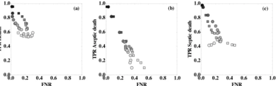
To obtain more detailed information about the performance of the classifier, we also studied the true positive rates (TPR) and false negative rates (FNR) for each steady-state outcome (health, aseptic death, and septic death) for model (1) (Fig 7). We find that high true positive
Fig 6. Prediction accuracy of the steady-state outcome as a function of patient variation.The prediction accuracyAusing a logistic regression classifier at timetc= 0 (symbols) and the average best
guess over 103initial conditions (dashed curves) versus patient variationvfor (a) models (1) and (2), (b) models (3) and (4), and (c) models (5) and (6).
doi:10.1371/journal.pone.0135861.g006
Fig 7. True positive rates versus false negative rates as a function of the prediction accuracy for model (1).True positive rates (TPR) for each outcome, (a) health, (b) aseptic death, and (c) septic death, versus the false negative rates (FNR) for model (1). For the FNR in (a), squares (circles) indicate that the outcome was health, but the prediction was aseptic death (septic death). For the FNR in (b), squares (circles) indicate that the outcome was aseptic death, but the prediction was health (septic death). For the FNR in (c), squares (circles) indicate that the outcome was septic death, but the prediction was health (aseptic death). The intensity of the shading of each symbol represents the prediction accuracy and scales linearly from
A= 1.0 (black) to 0.33 (white), which is obtained from random guessing.
rates are strongly correlated with high prediction accuracyA. As the accuracy decreases, the TPR decreases and FNR increases.Fig 7(b)also shows that one reason for low prediction accu-racy at high patient variability is the difficulty of the classifier to identify aseptic death states as evidenced by the low TPR values.
We further investigated the influence of a different parameter sampling method on the pre-diction accuracy.Fig 8compares the sampling of parameters of model (1) inFig 6to the sam-pling with a log-normal distribution instead of with a truncated normal distribution.Fig 8(a) shows the prediction accuracy versus patient variability data of model (1) inFig 6for sampling with truncated normal and log-normal distributions. In all cases the means and the standard deviations of the two distributions are the same. For smallv, the distributions are very similar and hence the prediction accuracies are very similar. For increasingvthe distributions differ more (panels (b)—(d)). Therefore the sampling of states differs, and with it there is a larger dis-crepancy in the prediction accuracy.
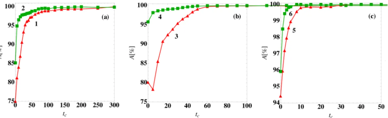
InFig 6, we showed results for the logistic regression prediction method with classification attc= 0. InFig 9, we show the prediction accuracy for models (1)-(6) with patient variability
v= 0.05 as a function of the classification timetc. For all models, the prediction accuracy grows
Fig 8. Comparison of the prediction accuracy for patient parameter variability sampled from normal and log-normal distributions.(a) Prediction accuracyAversus parameter coefficient of variationvfor model (1) and classification timetc= 0 with parameters sampled from a truncated Gaussian (red triangles)
and log-normal (green squares) distributions. Sample Gaussian (dashed red) and log-normal (solid green) parameter probability distributionsP(q) with meanμand coefficient of variation (b)v= 0.05, (c) 0.2, and (d) 0.5. For smallv, the Gaussian and log-normal distributions overlap. Forv0.5, the two distributions begin to differ nearq= 0 andqμ.
doi:10.1371/journal.pone.0135861.g008
Fig 9. Prediction accuracy of the steady-state outcome as a function of the classification time.The prediction accuracyAusing a logistic regression classifier at timetc(symbols) for (a) models (1) and (2), (b) models (3) and (4), and (c) models (5) and (6) for patient variationv= 0.05.
with increasingtc, reaching nearly 100% beyond a characteristic timetthat depends on the model. The prediction accuracy improves at later classification times because the system trajec-tories have moved closer to the fixed points and hence the basins of attraction are more easily separated as shown inFig 1for model (1).
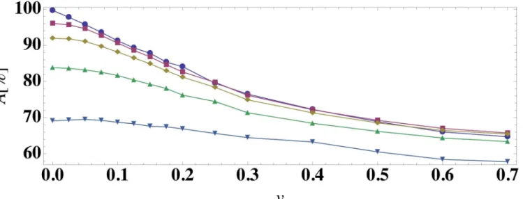
We also investigated the variation of the prediction accuracy in the presence of measure-ment noise. We took the trajectories generated forFig 6and added Gaussian random noise to the model variables with variancesat each time point. We then performed training and testing on the noisy data with classification at timetc= 0. InFig 10, we show for model (6) that the pre-diction accuracy decreases with increasings. We find similar results for models (1)-(5). These results emphasize that even if the measurement noise could be reduced to zero, the patient vari-ation imposes an intrinsic limitvari-ation to outcome prediction.
Discussion
In clinical settings it is of great importance to determine patient outcomes as quickly as possible with maximum accuracy. In this manuscript, we studied the effects of patient variability on the ability to predict steady-state outcomes in systems of ODEs that model the immune response to infection. For deterministic systems of ODEs with a given fixed set of parameters, each initial condition can be mapped to a given steady-state outcome (or fixed point) and the collection of initial conditions that map to a given steady-state outcome is defined as the basin of attraction of that outcome. Each virtual patient can be defined by a given set of parameters in the model ODE and patient variability can be introduced by varying the model parameters.
We showed that the introduction of patient variation leads to overlaps of the basins of attraction for the steady-state outcomes. In particular, a given initial condition can map to mul-tiple steady-state outcomes for different virtual patients (i.e. v>0), which is similar to the case of patients showing different responses to infection in clinical settings. We find that the predic-tion accuracy of the outcomes decreases strongly with increasing patient variability. Our results emphasize that even when the complete state of the system is known (i.e.all patient variables
Fig 10. Prediction accuracy as a function of patient variation for different noise strengths.The prediction accuracyAusing a logistic regression classifier at timetc= 0 for model (6) in the presence of measurement noise with strengths= 0 (circles), 0.05 (squares), 0.10 (diamonds), 0.20 (triangles), and
0.50 (triangles).
are measured precisely as a function of time), we have limited knowledge of the patient out-come when there is patient-to-patient variability that gives rise to basin overlap.
Our results also show that for all of the model ODEs studied the prediction accuracy increases as the timetcused for classification increases. Astcincreases, the systems move closer to their steady-state outcomes and the basins of attraction separate, which increases the predic-tion accuracy. Again, this result is consistent with clinical experience. If a clinician waits to see if the condition of the patient improves or worsens, the prognosis will become more accurate. In our work, we explicitly show that patient-to-patient fluctuations cause a competition between early and accurate outcome prediction.
In this work, we focused on discrete steady-state outcomes (i.e.health or death of the patient) of the immune response to infection. However, in many biomedical scenarios, the out-comes involve continuous variables rather than discrete states. In future work, we will apply similar techniques to understand the effects of patient variability on the predictions of continu-ous model variables, for example, the immune response and vaccination efficacy for influenza [28].
Another important future direction is to combine outcome prediction with a treatment regi-men. Treatments will depend on the predicted outcome,e.g.treatment for septic death would involve an antibiotic, while treatment for aseptic death would incorporate an immune suppres-sor. The predicted outcome can be updated based on the response of the patient to the treat-ment, and a new treatment can be identified based on the new prediction.
Acknowledgments
This work was partially supported by DARPA (Space and Naval Warfare System Center Pacific) under award number N66001-11-1-4184 and partially supported by the National Sci-ence Foundation Grant No. NSF PHY11-25915. Additional support for this work was provided by the Infectious Disease Supercluster, Colorado State University, 2012 seed grant. This work also benefited from the facilities and staff of the Yale University Faculty of Arts and Sciences High Performance Computing Center and NSF Grant No. CNS-0821132 that partially funded acquisition of the computational facilities.
Author Contributions
Conceived and designed the experiments: MM KW MS MK GH CO. Performed the experi-ments: MM. Analyzed the data: MM. Contributed reagents/materials/analysis tools: MM MS. Wrote the paper: MM MS CO.
References
1. Koup RA, Safritt JT, Cao Y, Andrews CA, McLeod G, Borkowsky W, et al. Temporal association of cel-lular immune responses with the initial control of viremia in primary Human Immunodeficiency Virus Type 1 Syndrome. J Virol. 1994; 68(7): 4650–4655. PMID:8207839
2. Guidotti LG, Chisari FV. Noncytolytic control of viral infections by the innate and adaptive immune response. Annu Rev Immunol. 2001; 19(1): 65–91. doi:10.1146/annurev.immunol.19.1.65PMID: 11244031
3. Janeway CA Jr, Medzhitov R. Innate immune recognition. Annu Rev Immunol. 2002; 20(1): 197–216. doi:10.1146/annurev.immunol.20.083001.084359PMID:11861602
4. Klipp E. Systems Biology in Practice: Concepts, Implementation And Application. 1st ed. Weinheim: Wiley-VCH; 2005.
6. Pope C, Kim SK, Marzo A, Williams K, Jiang J, Shen H, et al. Organ-specific regulation of the CD8 T cell response to Listeria monocytogenes infection. J Immunol. 2001; 166(5): 3402–3409. doi:10.4049/ jimmunol.166.5.3402PMID:11207297
7. Young D, Stark J, Kirschner D. Systems biology of persistent infection: Tuberculosis as a case study. Nat Rev Microbiol. 2008; 6(7): 520–528. doi:10.1038/nrmicro1919PMID:18536727
8. Castillo-Chavez C, Feng Z. To treat or not to treat: the case of tuberculosis. J Math Biol. 1997; 35: 629–656. doi:10.1007/s002850050069PMID:9225454
9. Perelson AS, Nelson PW. Mathematical analysis of HIV-1 dynamics in vivo. SIAM Rev. 1999; 41(1), 3–44. doi:10.1137/S0036144598335107
10. Callaway DS, Perelson AS. HIV-1 infection and low steady state viral loads. B Math Biol. 2002; 64(1): 29–64. doi:10.1006/bulm.2001.0266
11. Nelson PW, Perelson AS. Mathematical analysis of delay differential equation models of HIV-1 infec-tion. Math Biosci. 2002; 179(1): 73–94. doi:10.1016/S0025-5564(02)00099-8PMID:12047922 12. Perelson AS. Modeling viral and immune system dynamics. Nat Rev Immunol. 2002; 2(1): 28–36. doi:
10.1038/nri700PMID:11905835
13. Perelson AS, Neumann AU, Markowitz M, Leonard JM, Ho DD. HIV-1 dynamics in vivo: Virion clear-ance rate, infected cell life-span, and viral generation time. Science. 1996: 271: 1582–1586. doi:10. 1126/science.271.5255.1582PMID:8599114
14. Bocharov GA, Romanyukha AA. Mathematical model of antiviral immune response III. Influenza A virus infection. J Theor Biol. 1994; 167(4): 323–360. doi:10.1006/jtbi.1994.1074PMID:7516024
15. Belz GT, Wodarz D, Diaz G, Nowak MA, Doherty PC. Compromised influenza virus-specific CD8+-T-cell memory in CD4+-T-CD8+-T-cell-deficient mice. J Virol.2002; 76(23): 12388–12393. doi:10.1128/JVI.76.23. 12388-12393.2002PMID:12414983
16. Dowdy DW, Chaisson RE, Moulton LH, Dorman SE. The potential impact of enhanced diagnostic tech-niques for tuberculosis driven by HIV: A mathematical model. Aids 2006; 20(5): 751–762. doi:10.1097/ 01.aids.0000216376.07185.ccPMID:16514306
17. Wodarz D, Nowak MA. Mathematical models of HIV pathogenesis and treatment. BioEssays. 2002; 24(12): 1178–1187. doi:10.1002/bies.10196PMID:12447982
18. Serdobova I, Kieny MP. Assembling a global vaccine development pipeline for infectious diseases in the developing world. Am J Public Health. 2006 September; 96(9): 1554–1559. doi:10.2105/AJPH. 2005.074583PMID:16873743
19. Wetterstrand KA. DNA Sequencing Costs: Data from the NHGRI Genome Sequencing Program (GSP) Available at:www.genome.gov/sequencingcosts. Accessed Jan. 2015.
20. Day J, Rubin J, Vodovotz Y, Chow CC, Reynolds A, Clermont G. A reduced mathematical model of the acute inflammatory response II. Capturing scenarios of repeated endotoxin administration. J Theor Biol. 2006; 242(1): 237–256. doi:10.1016/j.jtbi.2006.02.015PMID:16616206
21. Vodovotz Y., Csete M., Bartels J., Chang S., & An G. Translational systems biology of inflammation. PLoS Comput Biol. 2008; 4(4): e1000014. doi:10.1371/journal.pcbi.1000014PMID:18437239 22. Vodovotz Y, Constantine G, Rubin J, Csete M, Voit EO, An G. Mechanistic simulations of inflammation:
Current state and future prospects. Math Biosci. 2009; 217(1): 1–10. doi:10.1016/j.mbs.2008.07.013 PMID:18835282
23. Webb GF, D’Agata EMC, Magal P, Ruan S. A model of antibiotic-resistant bacterial epidemics in hospi-tals. P Natl Acad Sci USA. 2005; 102: 13343–13348. doi:10.1073/pnas.0504053102
24. Wang K, Bhandari V, Chepustanova S, Huber G, Stephen O, Corey SO, et al. Which biomarkers reveal neonatal sepsis?. PLoS One 2013; 8(12): e82700. doi:10.1371/journal.pone.0082700PMID: 24367543
25. O’Hara S, Wang K, Slayden RA, Schenkel AR, Huber G, O’Hern CS, et al. Iterative feature removal yields highly discriminative pathways. BMC Genomics. 2013; 14(1): 832. doi: 10.1186/1471-2164-14-832PMID:24274115
26. Reynolds A, Rubin J, Clermont G, Day J, Vodovotz Y, Bard Ermentrout G. A reduced mathematical model of the acute inflammatory response: I. Derivation of model and analysis of anti-inflammation. J Theor Biol. 2006; 242(1): 220–236. doi:10.1016/j.jtbi.2006.02.016PMID:16584750
27. Hastie T, Tibshirani R, Friedman J. The elements of statistical learning. New York: Springer; 2009. 28. Hancioglu B, Swigon D, Clermont G. A dynamical model of human immune response to Influenza A