Ann. Geophys., 27, 2925–2936, 2009 www.ann-geophys.net/27/2925/2009/
© Author(s) 2009. This work is distributed under the Creative Commons Attribution 3.0 License.
Annales
Geophysicae
Solar stereoscopy – where are we and what developments do we
require to progress?
T. Wiegelmann1, B. Inhester1, and L. Feng1,2
1Max-Planck-Institut f¨ur Sonnensystemforschung, Max-Planck-Strasse 2, 37191 Katlenburg-Lindau, Germany 2Purple Mountain Observatory, Chinese Academy of Sciences, 210008, Nanjing, China
Received: 19 May 2009 – Revised: 13 July 2009 – Accepted: 17 July 2009 – Published: 23 July 2009
Abstract. Observations from the two STEREO-spacecraft give us for the first time the possibility to use stereoscopic methods to reconstruct the 3-D solar corona. Classical stere-oscopy works best for solid objects with clear edges. Con-sequently an application of classical stereoscopic methods to the faint structures visible in the optically thin coronal plasma is by no means straight forward and several problems have to be treated adequately: 1) First there is the problem of identifying one-dimensional structures – e.g. active region coronal loops or polar plumes- from the two individual EUV-images observed with STEREO/EUVI. 2) As a next step one has the association problem to find corresponding structures in both images. This becomes more difficult as the angle between STEREO-A and B increases. 3) Within the recon-struction problem stereoscopic methods are used to compute the 3-D-geometry of the identified structures. Without any prior assumptions, e.g., regarding the footpoints of coronal loops, the reconstruction problem has not one unique solu-tion. 4) One has to estimate the reconstruction error or ac-curacy of the reconstructed 3-D-structure, which depends on the accuracy of the identified structures in 2-D, the separa-tion angle between the spacecraft, but also on the locasepara-tion, e.g., for east-west directed coronal loops the reconstruction error is highest close to the loop top. 5) Eventually we are not only interested in the 3-D-geometry of loops or plumes, but also in physical parameters like density, temperature, plasma flow, magnetic field strength etc. Helpful for treating some of these problems are coronal magnetic field models extrap-olated from photospheric measurements, because observed EUV-loops outline the magnetic field. This feature has been used for a new method dubbed “magnetic stereoscopy”. As examples we show recent application to active region loops.
Correspondence to:T. Wiegelmann ([email protected])
Keywords. Solar physics, astrophysics,and astronomy (Corona and transition region; Magnetic fields; Ultraviolet emissions)
1 Introduction
within this paper we would like to give a review on what has been done in solar stereoscopy so far, which developments are currently under consideration, and planned for the future. The key question is how we can derive the 3-D geome-try and physical structure of the solar corona from images observed with the two STEREO-spacecraft? In Sect. 2 we describe a step by step guide, which contains the identifica-tion of curvi-linear structures from coronal EUV-images in Sect. 2.1, the association of the identified structures in both images from different vantage viewpoints in Sect. 2.2, the geometric 3-D stereoscopy (Sect. 2.3) and estimation of the 3-D-reconstruction error in Sect. 2.4. After these steps one has obtained the 3-D geometry of, e.g., active region loops or polar plumes and in Sect. 2.5 we outline how physical quantities like temperature and density can be found. An in-teresting question, which we address in Sect. 3, is how well do stereoscopic reconstructed plasma loops agree with coro-nal magnetic field models? Due to the high conductivity of the coronal plasma the magnetic field is outlined by the radi-ating plasma and in principle one has two independent data sources about the 3-D geometry of coronal loops, namely stereoscopy and magnetic field extrapolations from photo-spheric measurements. In Sect. 4 we address how in future stereoscopic, tomographic and self-consistent modelling ap-proaches could be combined and diminish weaknesses of the individual approaches.
2 Step by step guide to stereoscopy
2.1 Extraction of curvi-linear objects from EUV-images
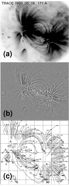
A first step for stereoscopy is to extract curve-like structures (projections of coronal loops) from observed EUV-images such as from the TRACE-image shown in Fig. 1a). A prin-cipal problem of identifying loops is that the solar corona is optically thin and the loops are faint. Visible loops are often a superposition of multiple individual loops (Schrijver et al., 1999, 2004). Figure 1b shows the TRACE-image af-ter a 7×7-boxcar smoothed image was removed from the original, which enhances the contrast. Aschwanden et al. (2008a) manually traced 210 loops as shown in panel (c). While hand-tracing might be suitable to investigate a few individual cases, this is not appropriate to study large data sets and time sequences. Several automatic feature recogni-tion methods have been developed. The example shown in Fig. 1 has been used to compare and evaluate five automated loop segmentation methods. The output of the five codes has been compared with the hand-traced loops from Fig. 1c. This comparison revealed large differences. The codes iden-tified between 76 and 347 loops. Among the longer and more significant loops, the various codes identified between 19% and 59% of the corresponding 154 hand traced loops above this limit. Some codes wrongly identified noise as spuri-ous short loops. Obvispuri-ously the state-of-the-art of automatic
(
a
)
(
b
)
(
c
)
T. Wiegelmann et al.: Coronal stereoscopy 2927
Fig. 2.Top: Contrast enhanced EUVI images from STEREO-B (left) and A (right) of the NOAA AR 0960 on 8 June 2007. The individual loops (enumerated white curves) have been extracted by a semi-automatic feature recognition tool as described in Inhester et al. (2008). Please note that equal numbers do not imply a correspondence across the images. Bottom: Some selected coronal loops (yellow) with their best fit magnetic field line (red). The separation angle between the spacecraft was 12◦(the top figures have been published originally in Feng et al., 2007b, Fig. 1).
feature recognition techniques is not satisfactory. The indi-vidual codes have control parameters, adapted to the image signal to noise ratio, resolution and also to the type of ob-jects it aims to extract. A prime problem is that time-varying background loops and moss prevent an uncontaminated sepa-ration of loop and background. This makes it difficult to trace loop tops and footpoints. The problem becomes more com-plex for the comparison of EUV-images taken at different wavelengths and temperatures because the background is dif-ferent in each filter. In the current stage the automatic feature recognition tools are already useful, but some human interac-tion is usually necessary and the codes can be considered as semi-automatic. The automated segmentation of polar
plumes as stationary objects whose intensity varies homoge-neously with time.”). Two STEREO-viewpoints are expected to be most useful for the tomography of plumes when the separation angle is about 60◦.
2.2 Association of objects in both images
For faint objects like coronal EUV-loops it is not trivial to find associated structures in images taken from different van-tage points as shown in Fig. 2. Rodriguez et al. (2009) de-veloped a correlation tracking method which automatically matches pixels in both images, which worked well for small separation angles between spacecraft but it becomes difficult and ambiguous for if the separation angle of the spacecraft exceeds about 15◦. In particular for large separation
an-gles some structures might be visible in one image, but not in the other. Aschwanden et al. (2008c) applied a forward projection with an assumed height range ofh=0...0.1Rs, which was sufficient to find correspondence for 30 traced loop, when the separation angle between STEREO-A and B was only 7◦. The correspondence problem becomes more difficult to solve for larger separation angles.
Other possibilities are the use of a priori assumptions of the coronal structures, e.g., fitting to a semi-circular loop model (Aschwanden et al., 1999), or loop curvature con-straints (Aschwanden, 2005). As an alternative one can use the fact that the emitting EUV-radiation outlines mag-netic field lines due to the high conductivity of the coronal plasma. Consequently magnetic field lines should provide a reasonable proxy for coronal plasma loops. Wiegelmann and Neukirch (2002) used the stereoscopic reconstructed loops from Aschwanden et al. (1999) and photospheric mag-netograms from SOHO/MDI to fit the optimum parameter
αwithin the linear force-free field approximation. Projec-tions of extrapolated 3-D magnetic field lines under different model assumptions have been compared with coronal im-ages in Gary and Alexander (1999); Carcedo et al. (2003); R´egnier and Amari (2004); Wiegelmann et al. (2005). The method has been extended for a STEREO pair of EUV-images in combination with linear and nonlinear force-free field models in Wiegelmann and Inhester (2006) and was dubbed magnetic stereoscopy. The idea of magnetic stere-oscopy is that a number of 3-D field line proxies are projected onto the EUV-images and compared with the corresponding extracted curve-like structures (see Sect. 2.1). Loops in both images which have a minimum distance to the projection of a 3-D magnetic field line are very likely related to each other. The field line proxies where generated from extrapola-tion models but any other method to produce parameterized meaningful 3-D curves would work as well. The extrapo-lation models are here just a convenient means to generate 3-D curves the observed loops can be compared with. The method has been applied to TRACE-data (taken a day apart) by Feng et al. (2007b) and to STEREO/SECCHI by Feng et al. (2007a). In both cases the magnetic field has been
com-puted with the linear force free method developed by See-hafer (1978) from SOHO/MDI. Force-free fields are charac-terized by∇ ×B=αBandB· ∇α=0, whereB is the mag-netic field andαis zero for potential fields and constant in the entire space for linear force-free models. For more sophisti-cated non-linear force-free field models,αis constant along field lines but may vary on different field lines. An advantage of using coronal magnetic field models is that they generate meaningful and physics-based 3-D curves. Note, however, that a set of field lines from a linear force-free model con-structed with a differentαdoes not constitute a physically consistent magnetic field model. Disadvantages are that one needs additional observations from ground-based or space-borne magnetographs (a third eye, e.g., SOHO or in future SDO) and that magnetic modelling and stereoscopy are not independent from each other, which is helpful for evaluat-ing the consistency of both methods (see also discussion in Sect. 3).
2.3 Geometric stereoscopy
T. Wiegelmann et al.: Coronal stereoscopy 2929
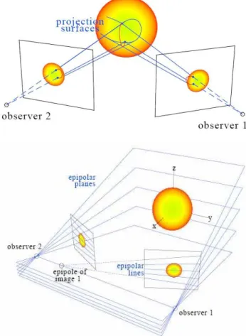
Fig. 3. Top panel: Back projection to reconstruct curve-like ob-jects, e.g., coronal loops, from two images. Bottom panel: Epipolar planes and the corresponding epipolar lines in two STEREO-images (top and bottom panel of this figure have been originally published in Inhester, 2006, Figs. 1 and 2, respectively).
height in the corona. A simple way to tie-point associated loop curves in image A and B is to label along each curve the intersections with given epipolar lines and to reconstruct the intersection points with the same epipoles line label. This, of course, requires that both curves cover more or less the same epipolar range, a criterion which can be used to confirm a correct association.
2.4 Estimating the reconstruction error in 3-D
Features in the two STEREO-images can be identified of course only within a certain error margin as indicated by
win Fig. 4 top panel. Possible error sources are the finite resolution of the instrument as well as uncertainties occur-ring due to extracting features from the EUV-images. The question is how do these uncertainties in the 2-D-images af-fect the reconstruction error of the 3-D coronal loop? As a consequence of the finite resolution w of the loop pro-jection, the true 3-D coordinate of a loop point lies nearby
Fig. 4. Top: How does the uncertainty w of the projected loop in both EUV-images affect the error-trapezoid of the recon-structed 3-D-loop? (see text) (original publishes in Inhester, 2006, Fig. 10), Bottom: Stereoscopic reconstructed 3-D loop (yellow) and best fit linear force free coronal magnetic field line extrapolated from SOHO/MDI magnetograms (original published in Feng et al., 2007a, Fig. 5).
in a plane through the reconstructed point which is spanned by the local normalsni of the two projection surfaces. t=
(n1×n2)/|n1×n2|is the local curve tangent. Decomposing the uncertainty vector into its componentsn1andn2 yields an error trapezoid of the positional uncertainty has the axes
w/(2cos(α/2)) and w/(2sin(α/2)), where α is the angle between the projection surface normals (see Inhester, 2006, for a mathematical derivation and more details). For small
αthe depth error along the mean view direction of the two spacecraft may be considerable: 1/(2sin(α/2))exceeds 5 for
α <10◦. αis limited from above by the angle between the
Fig. 5.Stereoscopic reconstructed 3-D loops and sections of loops (yellow) and best fit linear force-free field lines (red) from differ-ent viewpoints (top panel: view from STEREO-A, bottom panel: Northeast of the Active Region). (Original published in Feng et al., 2007a, Figs. 3 and 4.)
error bars in Fig. 4 bottom panel, which shown a stereoscopic reconstruction of one loop from (Feng et al., 2007a) for a separation angle of 12◦between spacecraft. A small (large)
separation angle between spacecraft makes it easy (difficult) to associate related structures in both images, but for the 3-D reconstruction error it is the other way around, a small sepa-ration angle leads to a large error in 3-D.
An alternative error estimate has been given by Aschwan-den et al. (2008c) for the uncertainty in height. Both error estimates show a similar behaviour, however: The smallest error is obtained if the loop tangent is normal to the epipo-lar planes and the error becomes infinite if the loop tangent becomes parallel to the epipolar plane.
Another problem in finding a unique solution for the 3-D loop is a possible reconstruction ambiguity. This is a problem which can theoretically occur even for a pair of correctly identified loop projections, if the footpoints are wrongly associated in the image pair. In EUV images, the footpoints of loops are sometimes difficult to locate. They may be drowned in bundles of other loops or near-surface
EUV moss. This problem does, however, disappear if one can identify the footpoints of loops and requires them to be located near the solar surface. It is, however, not always pos-sible to identify the loop footpoints and in this case one has two possible candidates for the true 3-D-solution. The true and the false reconstruction intersect at a point, where the projected segment is parallel to an epipolar line, e.g., the top of east-west coronal loops where the above error estimate formally diverges.
How can ambiguities and errors be limited? One possi-bility would be to use additional EUV-images from a third viewpoint, e.g., SOHO/EIT or in future SDO/AIA. This pos-sibility has (to our knowledge) not been tried out yet. A potential problem might be the different resolution of the STEREO/SECCHI-EUVI and the SOHO/EUV instruments. The error in line-tying is also reduced by making use of the fact that the reconstructed loops should resemble field lines and hence should be smooth. Smoothing and/or spline fitting of the tie point reconstruction should in general reduce the reconstruction error.
Another possibility, which has been already shown to be useful for the association problem (Sect. 2.2), is to use coro-nal magnetic field models. This possibility, called “magnetic stereoscopy” was first tested with a model active region in Wiegelmann and Inhester (2006). Different magnetic field models, potential, linear and non-linear force-free have been used and it was shown that even the use of a poor field model (potential fields) was sufficient to resolve the reconstruction ambiguity. The extrapolated magnetic field lines provide al-ready a proxy for the 3-D plasma loop and if ambiguous solu-tions occur, the solution closer to this proxy-loop is chosen. Figure 4 bottom panel and Fig. 5 shows a linear force-free field line (extrapolated from SOHO/MDI) in red, which has been used for this aim in Feng et al. (2007a). Extrapolated field lines might also serve as a reasonable approximation of the plasma loop in regions with a large reconstruction error, e.g., the loop top or if only parts of the loop are visible in the EUV-images.
2.5 Derive physical quantities
The geometry of the 3-D coronal structures, as seen from dif-ferent viewpoints in Fig. 5 in yellow provide already useful information. Feng et al. (2007a) found that most of the recon-structed 3-D loops cannot be approximated by planar curve segments and that most of the loops are not circular. This was already known from field modelling. E.g. meaningful loop emissions per unit loop length can only be derived from EUV images, if the angle between the viewing direction and the loop tangent is properly taken into account (Aschwanden et al., 2008b).
T. Wiegelmann et al.: Coronal stereoscopy 2931
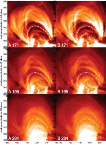
Fig. 6.EUVI-images at different wavelengths from STEREO-A and B in the left and right panels, respectively. The dashes white line shows a projections of a 3-D loop as reconstructed in (Aschwanden et al., 2008c). (Original published in Aschwanden et al., 2008b, Fig. 1).
(Aschwanden et al., 2008c) onto STEREO/SECCHI images at different wavelengths taken from STEREO-A and B in the left and right panels, respectively. As explained in detail in (Aschwanden et al., 2008b) the EUVI-images can be used to obtain the electron temperature and density, independent of each other for the EUVI-images taken from both STEREO-viewpoints, which have been separated by 7◦for this study.
As only a fraction of about 10% of the EUV-radiation is com-ing from the loops, one has to remove first the background separately in each wavelength, which is a tricky busyness and requires model assumptions as explained in detail in (As-chwanden et al., 2008b). After the well known temperature response functions (defined for each wavelength), as calcu-lated with the CHIANTI-code, are used to obtain physical quantities along the loops. For this aim a local loop-aligned coordinate system is introduced and the differential emission measure (DEM) is constrained for each loop position with 3 temperature filters at various positions along the loop with a Gaussian function. The DEM is then fitted with the help of the EUVI response functions in three wavelength, which
pro-Fig. 7. Temperature map of 30 loops. The loops are isothermal within the error estimation and the hottest loops are also the small-est. (Original published in Aschwanden et al., 2008b, as part of Fig. 9).
Wiegelmann et al.: Coronal stereoscopy
Where to go in stereoscopy?
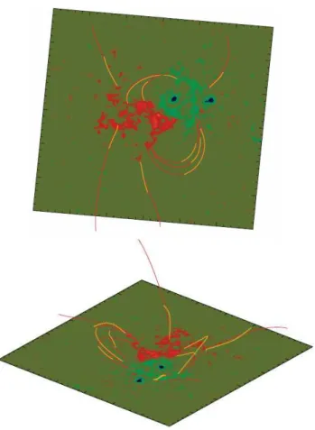
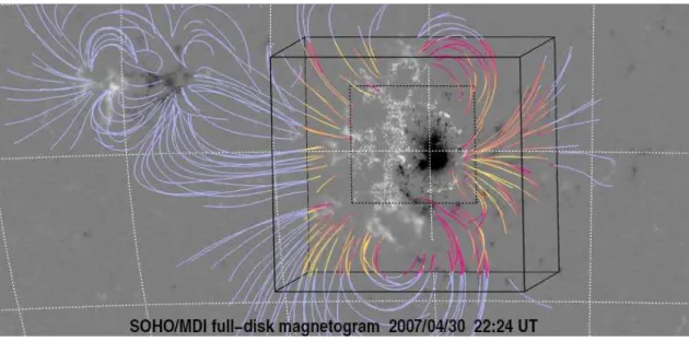
Fig. 8.SOHO/MDI magnetogram of AR 10953 with over-plotted stereoscopic reconstructed loops (see Aschwanden et al., 2008c) in blue and extrapolated non-linear force-free coronal magnetic field lines. The solid box depicts the 320×320×256 grid point simulation box in which the magnetic field extrapolations have been carried out. The dotted area depicts the field-of-view of Hinode/SOT-SP. Only in this dotted area photospheric vector magnetograms have been available. (Original published in DeRosa et al., 2009, as part of Fig. 1).
3 Stereoscopy and coronal modelling
As explained in the previous section, coronal magnetic field models provide useful information for solving the stereo-scopic correspondence problem (see Sect. 2.2) and to remove reconstruction ambiguities (Sect. 2.4). Until now mainly lin-ear force-free models have been used for this aim and the method automatically fits the optimum linear force-free pa-rameterαfor each loop individually to approximate its shape as closely as possible.αis here just used as a numerical pa-rameter to alter the curve shape. It is therefore not surprising that Feng et al. (2007a) found a significant scatter ofα be-tween the loops. We cannot interpret the values ofαin terms of a linear force-free magnetic field model, because the dif-ferent values are a contradiction to the premises of a globally constantα. For a physical meaningful self-consistent mag-netic field model one cannot determine the values ofα inde-pendently for each loop. Unfortunately, a physical consistent nonlinear model is way more demanding, both computation-ally due to the intrinsic nonlinearity of the model and from an observational point of view since nonlinear models re-quire photospheric vector magnetograms as input. Within the last few years a group of scientists (nonlinear force-free field consortium, chaired by C. Schrijver) has intensively com-pared and evaluated corresponding computer codes (Schri-jver et al., 2006, 2008; Metcalf et al., 2008), which showed the codes produce reliable results, when feeded with con-sistent input data (vector magnetograms or a quantity de-rived from vector magnetograms). In another joint study of the consortium (by DeRosa et al., 2009) the codes have
been applied to AR 10953 and the 3-D structure of the mag-netic field lines has been compared with the 3-D geometry of plasma loops (as stereoscopically reconstructed in Aschwan-den et al., 2008c). Figure 8 shows the stereo-loops in blue and in red and yellow the magnetic field lines. A major diffi-culty of this study was that the Hinode-SOT/SP vector mag-netograms, required as input for the magnetic field codes, where available in only a very small field of view (dotted area in Fig. 8) and has only about 10% of the area spanned by the stereo loops. The majority of stereo-reconstructed loops were located outside of this region, therefore the reconstruc-tion box was significantly enlarged beyond the Hinode-area (solid lines in Fig. 8, but only the line of sight component of the photospheric magnetic field from SOHO/MDI was avail-able in this enlarged box. Assumptions regarding the trans-verse photospheric field component had to be made in the MDI-area, but unfortunately the various magnetic field codes made different use of the assumption in the MDI-area and consequently the resulting magnetic field lines differed be-tween the codes. The extrapolated magnetic field lines turned out to be also inconsistent with the reconstructed STEREO-loops. There was an average misalignment angle of 24◦
T. Wiegelmann et al.: Coronal stereoscopy 2933 actually vector magnetogram data have been available and
correspondingly the codes have not been fed with a consis-tent input. As visible in Fig. 8 almost no field line/STEREO-loop closes within the Hinode field of view. It is therefore necessary to repeat such a study with much larger field of view of vector magnetogram data (ideally at least the same FOV as spanned by the STEREO-loops).
An additional complication is that the magnetic field vec-tor is measured routinely only in the photosphere, where the magnetic field is not force-free due to the high plasma β
(see Metcalf et al., 1995). Consequently photospheric vec-tor magnetograms do not provide consistent boundary con-ditions for a nonlinear force-free extrapolation. To over-come this difficulty, a preprocessing method has been de-veloped to remove the non-magnetic forces from the photo-spheric vector magnetograms (see Wiegelmann et al., 2006; Fuhrmann et al., 2007, for details). These preprocessed magnetograms are more chromospheric like and chromo-spheric observations, e.g., can be incorporated into the preprocessing-algorithm as described in Wiegelmann et al. (2008). In principle one could incorporate additional obser-vational constraints into the preprocessing routine, for exam-ple minimize the angle of stereoscopic reconstructed loops (at the footpoints) with the magnetic field vector. This might help to better estimate the magnetic field vector in the upper chromosphere. Another possibility which might be tried out is to add a term which minimizes the angle between the coro-nal magnetic field and the reconstructed 3-D corocoro-nal loops in the nonlinear force-free modelling algorithm. One possibil-ity would be to extend the nonlinear force-free optimization principle Wheatland et al. (2000); Wiegelmann (2004) by means of a Lagrangian multiplierζ as suggested in Eq. (1).
L=
Z
V
h
B−2|(∇ ×B)×B|2+ |∇ ·B|2id3V+
ζ
Z
V
(B×S3D)2d3V (1) The first two terms correspond to the force-free equations and the last term measures the angle between the coronal magnetic field B and the stereoscopic reconstructed 3-D-loopsS3D, whereS3D should contain also an error approx-imation of the stereoscopic reconstruction error This could be done by the local length of the vector S3D along the stereo-loop, where |S3D| =1 would indicate a small error and|S3D| =0 an infinite error. Locations with|S3D| =0 ob-viously do not contribute to the functional. The third term in Eq. (1) corresponds to a weighted angle between mag-netic field and STEREO-loops. Regions with high magmag-netic field strength and accurate measurement of|S3D|contribute more to the functional. As such data (an active region ob-served simultaneously by both STEREO-spacecraft and a large field-of-view vector magnetograph) seem not to be cur-rently available (also due to a lack of active regions in recent years), corresponding studies have to be postponed until af-ter the launch of SDO. The SDO/HMI intrument will
pro-vide full disc vectormagnetograph, which resolves the lim-ited FOV-problem of current instruments. However, the an-gle between the spacecraft might then be too large for stere-oscopy with STEREO A/B spacecraft. One has to evalu-ate whether SDO/AIA and one of the STEREO-spacecraft can be used for stereoscopy instead. The result can then be compared with nonlinear force-free extrapolations from SDO/HMI. This instrument will provide the required larger FOV for the field modelling.
4 Where to go in coronal stereoscopy?
To summarize the current state of the art of coronal stere-oscopy we propose a concept of five steps, namely: feature extraction, association, geometric reconstruction, error ap-proximation and physical modelling. Several improvements are still possible for some of the steps, e.g., a fully auto-matic and reliable feature recognition method, investigations on how stereoscopy is still possible with larger separation angles between the spacecraft and if we can combine also STEREO with other missions, e.g., SDO. Some basic diffi-culties, e.g., the large reconstruction error on the top of east-west loop is an intrinsic problem of stereoscopy, unless we have one or more spacecraft well above or below the ecliptic. Despite these principal difficulties coronal stereoscopy provides us for the first time some information about the 3-D geometry and physical quantities of plasma loops. A useful concept has been also to combine stereoscopy with magnetic modelling of the solar corona, but due to shortage of vec-tor magnetogram data these approaches have been mainly done with linear force-free methods. With the forthcoming full disc vector magnetograph SDO/HMI nonlinear force-free magnetic field models are assumed to become avail-able on a regular basis. A principal problem of force-free magnetic field modelling is that it does not include a self-consistent modelling of the coronal plasma. Assume a static corona model for example, which balances the Lorentz-force with pressure gradient and gravity asj×B= ∇p+ρ∇ψ. The term force-free means that the Lorentz force vanishes and correspondingly the current densityj is parallel to the magnetic fieldB. While this approach is well justified for the field modelling in the low plasmaβsolar corona, it means also that∇p+ρ∇ψ=0, and because the gravity force−∇ψ
Self-consistent equilibrium
Artificial images LOS-integration
Where to go in stereoscopy?
Where to go in corona modeling?
Force-free
code
SDO/HMI magnetogramMHS
code
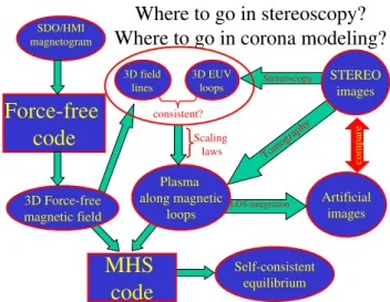
3D Force-free magnetic field 3D field lines compare Plasma along magnetic loops Scalinglaws Tomo graph y Stereoscopy STEREO images 3D EUV loops consistent?
Fig. 9.A concept on how stereoscopy could be imbedded in a self-consistent coronal modelling approach.
In Fig. 9 we outline an approach towards a self-consistent coronal modelling. First there should be two alternative routes to derive the 3-D geometry of coronal loops, either from two EUV-images by stereoscopy or by force-free ex-trapolations from vector magnetograms, e.g., as provided in future from SDO/HMI. The resulting 3-D field lines and 3-D EUV-loops should be consistent with each other. Unfortu-nately this has not been the case for a first comparison (by DeRosa et al., 2009) as discussed already in Sect. 3, but it is assumed (or at least hoped for)that the new instrumentation with SDO/HMI and improvements in modelling will lead to more consistent results. If consistency between plasma loops and field lines has been found, we will have a much more reliable magnetic field model than we obtain from extrapo-lation alone. One can then derive physical quantities along the loops as outlined in Sect. 2.5. An alternative method is to use a tomographic approach (as explained in detail in As-chwanden et al., 2009), which provides the plasma density without model assumptions. A sophisticated modelling of quantities along the loops can be done (see Schrijver et al., 2004, who used scaling laws between the photospheric mag-netic field and the heating rate at the footpoints of loops). From physical quantities like density and temperature one can compute artificial EUV-images and compare them with the real STEREO-images. This approach might as well al-low to adjust free parameters within the loop modelling ap-proach. As pointed out above, modelling of coronal magnetic field and plasma cannot be achieved a selfconsistently with a force-free model. Plasma loop modelling will create small gravity and plasma pressure forces, which have to be com-pensated by a Lorentz-forces. Due to the low coronal plasma
β, the Lorentz force required will be very small and the coro-nal magnetic field structure will deviate only margicoro-nally from a force-free model.
Finally a self-consistent model using the magneto-hydro-static approach can be computed with the force-free magnetic field model and the plasma along the loops as input. Cor-responding magneto-hydro-static codes have been developed and tested in Wiegelmann and Neukirch (2006); Wiegelmann et al. (2007) in cartesian and spherical geometry, respec-tively. The resulting consistent static model can be used as input to investigate dynamic phenomena for example with time-dependent MHD-codes.
With stereoscopically reconstructed loops, even if they are few in number, we will have for the first time an indirect though quantitative measurement of the local coronal mag-netic field direction. In future magmag-netic field extrapolation codes, this information should be used not only for a com-parison but as an additional constraint to lift some of the un-certainties which arise from unknown boundary values. For a forecast of the evolution and stability of observed active re-gions, we probably will need time dependent simulations of the corona which incorporate observations by data assimila-tion schemes similar to the way they are now used in compu-tational meteorology (see Daley, 1991). An anfolding of the solar remote sensing observations to constrain the 3-D state of the solar corona is vital for these schemes and the forecast range will strongly depend on the quality of the 3-D recon-structions. For this task, the techniques for detecting well defined objects in the images and the way they are processed into 3-D structures needs to be improved. The present state of the art of solar stereoscopy can only be a first step in this direction.
A challenging task in stereoscopy is the 3-D reconstruction of true dynamic phenomena like the initiation of flares and CMEs. A key question is which role magnetic reconnection plays for such eruptive phenomena. Stereoscopy could help us first to derive the quasi-stationary state before an eruption, preferably within a sophisticated self-consistent model, e.g., magneto-hydro-statics. If we can then also observe the 3-D-structure of the dynamic phase this would be very helpful for our understanding of such phenomena. One could, in partic-ular, use the self-consistent stationary state as input for time dependent simulations, e.g., with MHD or Hall-MHD. It is notoriously difficult to find transport coefficients, e.g., resis-tivity, viscosity, heat tensor etc. for the coronal plasma from micro-physics for the coronal plasma, because the required kinetic scales are way to small to observe. One could, how-ever, try to optimize these transport coefficient with a system-atic trial and error approach in order to fit the observations best. Such observational based simulations would provide us then a rich new world of insights. If the dynamic model simu-lations show reasonable agreement with observed quantities, we might also have some confidence in other model quan-tities, which cannot be observed. This could give insights about the physics of magnetic reconnection in the coronal plasma.
T. Wiegelmann et al.: Coronal stereoscopy 2935 be very helpful, together with high accuracy measurements
of the photospheric magnetic field vector, to understand the interface region between photosphere and corona. A phys-ical understanding of this region is important for the coro-nal heating problem. Corocoro-nal stereoscopy can help here be-cause it provides a fair approximation of the corona, but addi-tional direct observations of the interface region, as provided in near future for example from the small explorer mission IRIS are necessary. A modelling approach in this region is very challenging, because low and highβ plasma with sub-and supersonic plasma flows exist side by side here.
Acknowledgements. We would like to thank the organization com-mittee (chaired by Richard Harrison) of the STEREO-3/SOHO-22 workshop “Three eyes on the Sun” for the invitation to give this re-view on stereoscopy. This work was supported by DLR-grant 50 OC 0501. The SECCHI data used here were produced by an in-ternational consortium of the Naval Research Laboratory (USA), Lockheed Martin Solar and Astrophysics Lab (USA), NASA God-dard Space Flight Center (USA), Rutherford Appleton Laboratory (UK), University of Birmingham (UK), Max-Planck-Institut for So-lar System Research (Germany), Centre Spatiale de Li`ege (Bel-gium), Institut d’Optique Th`eorique et Appliqu`ee (France), and In-stitut d’Astrophysique Spatiale (France).
The service charges for this open access publication have been covered by the Max Planck Society.
Topical Editor R. Forsyth thanks two anonymous referees for their help in evaluating this paper.
References
Aschwanden, M. J.: 2D Feature Recognition And 3d Reconstruc-tion In Solar Euv Images, Sol. Phys., 228, 339–358, doi:10.1007/ s11207-005-2788-5, 2005.
Aschwanden, M. J., Newmark, J. S., Delaboudini`ere, J.-P., Ne-upert, W. M., Klimchuk, J. A., Gary, G. A., Portier-Fozzani, F., and Zucker, A.: Three-dimensional Stereoscopic Analysis of Solar Active Region Loops. I. SOHO/EIT Observations at Temperatures of (1.0–1.5) X 10ˆ6 K, ApJ, 515, 842–867, doi: 10.1086/307036, 1999.
Aschwanden, M. J., Alexander, D., Hurlburt, N., Newmark, J. S., Neupert, W. M., Klimchuk, J. A., and Gary, G. A.: Three-dimensional Stereoscopic Analysis of Solar Active Region Loops. II. SOHO/EIT Observations at Temperatures of 1.5–2.5 MK, ApJ, 531, 1129–1149, doi:10.1086/308483, 2000. Aschwanden, M. J., Lee, J. K., Gary, G. A., Smith, M., and
In-hester, B.: Comparison of Five Numerical Codes for Auto-mated Tracing of Coronal Loops, Sol. Phys., 248, 359–377, doi: 10.1007/s11207-007-9064-9, 2008a.
Aschwanden, M. J., Nitta, N. V., Wuelser, J.-P., and Lemen, J. R.: First 3D Reconstructions of Coronal Loops with the STEREO A+B Spacecraft. II. Electron Density and Temperature Measure-ments, ApJ, 680, 1477–1495, doi:10.1086/588014, 2008b. Aschwanden, M. J., W¨ulser, J.-P., Nitta, N. V., and Lemen, J. R.:
First Three-Dimensional Reconstructions of Coronal Loops with the STEREO A and B Spacecraft. I. Geometry, ApJ, 679, 827– 842, doi:10.1086/529542, 2008c.
Aschwanden, M. J., Wuelser, J.-P., Nitta, N. V., Lemen, J. R., and Sandman, A.: First Three-Dimensional Reconstructions of Coro-nal Loops with the STEREO A+B Spacecraft. III. Instant Stereo-scopic Tomography of Active Regions, ApJ, 695, 12–29, doi: 10.1088/0004-637X/695/1/12, 2009.
Barbey, N., Auch`ere, F., Rodet, T., and Vial, J.-C.: A Time-Evolving 3D Method Dedicated to the Reconstruction of Solar Plumes and Results Using Extreme Ultraviolet Data, Sol. Phys., 248, 409–423, doi:10.1007/s11207-008-9151-6, 2008.
Batchelor, D.: Quasi-stereoscopic imaging of the solar X-ray corona, Sol. Phys., 155, 57–61, 1994.
Berton, R. and Sakurai, T.: Stereoscopic determination of the three-dimensional geometry of coronal magnetic loops, Sol. Phys., 96, 93–111, 1985.
Carcedo, L., Brown, D. S., Hood, A. W., Neukirch, T., and Wiegel-mann, T.: A Quantitative Method to Optimise Magnetic Field Line Fitting of Observed Coronal Loops, Sol. Phys., 218, 29–40, 2003.
Daley, R.: Atmospheric Data Analysis, Cambridge Atmospheric and Space Science Series, 1991.
DeRosa, M. L., Schrijver, C. J., Barnes, G., Leka, K. D., Lites, B. W., Aschwanden, M. J., Amari, T., Canou, A., McTier-nan, J. M., R´egnier, S., Thalmann, J. K., Valori, G., Wheat-land, M. S., Wiegelmann, T., Cheung, M. C. M., Conlon, P. A., Fuhrmann, M., Inhester, B., and Tadesse, T.: A Critical As-sessment of Nonlinear Force-Free Field Modeling of the Solar Corona for Active Region 10953, ApJ, 696, 1780–1791, doi: 10.1088/0004-637X/696/2/1780, 2009.
Feng, L., Inhester, B., Solanki, S. K., Wiegelmann, T., Podlipnik, B., Howard, R. A., and Wuelser, J.-P.: First Stereoscopic Coronal Loop Reconstructions from STEREO SECCHI Images, ApJL, 671, L205–L208, doi:10.1086/525525, 2007a.
Feng, L., Wiegelmann, T., Inhester, B., Solanki, S., Gan, W. Q., and Ruan, P.: Magnetic Stereoscopy of Coronal Loops in NOAA 8891, Solar Phys., 241, 235–249, doi:10.1007/ s11207-007-0370-z, 2007b.
Feng, L., Inhester, B., Solanki, S. K., Wilhelm, K., Wiegelmann, T., Podlipnik, B., Howard, R. A., Plunkett, S. P., Wuelser, J. P., and Gan, W. Q.: Stereoscopic Polar Plume Reconstruc-tions from STEREO/SECCHI Images, ApJ, 700, 292–301, doi: 10.1088/0004-637X/700/1/292, 2009.
Fuhrmann, M., Seehafer, N., and Valori, G.: Preprocessing of solar vector magnetograms for force-free magnetic field extrapolation, A&A, 476, 349–357, doi:10.1051/0004-6361:20078454, 2007. Gary, G. A. and Alexander, D.: Constructing the Coronal Magnetic
Field By Correlating Parameterized Magnetic Field Lines With Observed Coronal Plasma Structures, Sol. Phys., 186, 123–139, 1999.
Helio-spheric Investigation (SECCHI), Space Sci. Rev., 136, 67–115, doi:10.1007/s11214-008-9341-4, 2008.
Inhester, B.: Stereoscopy basics for the STEREO mission, ArXiv Astrophysics e-prints, 2006.
Inhester, B., Feng, L., and Wiegelmann, T.: Segmentation of Loops from Coronal EUV Images, Solar Phys., 248, 379–393, doi:10. 1007/s11207-007-9027-1, 2008.
Kaiser, M. L., Kucera, T. A., Davila, J. M., St. Cyr, O. C., Guhathakurta, M., and Christian, E.: The STEREO Mission: An Introduction, Space Sci. Rev., 136, 5–16, doi:10.1007/ s11214-007-9277-0, 2008.
Llebaria, A., Thernisien, A., and Lamy, P.: Characterization of the polar plumes from high cadence LASCO-C2 observations, Adv. Space Res., 29, 343–348, doi:10.1016/S0273-1177(01)00595-6, 2002.
Metcalf, T. R., Jiao, L., McClymont, A. N., Canfield, R. C., and Uitenbroek, H.: Is the solar chromospheric magnetic field force-free?, ApJ, 439, 474–481, doi:10.1086/175188, 1995.
Metcalf, T. R., Derosa, M. L., Schrijver, C. J., Barnes, G., van Ballegooijen, A. A., Wiegelmann, T., Wheatland, M. S., Valori, G., and McTiernan, J. M.: Nonlinear Force-Free Modeling of Coronal Magnetic Fields. II. Modeling a Filament Arcade and Simulated Chromospheric and Photospheric Vector Fields, Solar Phys., 247, 269–299, doi:10.1007/s11207-007-9110-7, 2008. R´egnier, S. and Amari, T.: 3D magnetic configuration of the Hα
filament and X-ray sigmoid in NOAA AR 8151, A&A, 425, 345– 352, 2004.
Rodriguez, L., Zhukov, A. N., Gissot, S., and Mierla, M.: Three-Dimensional Reconstruction of Active Regions, Solar Phys., 256, 41–55, doi:10.1007/s11207-009-9355-4, 2009.
Rosner, R., Tucker, W. H., and Vaiana, G. S.: Dynamics of the quiescent solar corona, ApJ, 220, 643–645, doi:10.1086/155949, 1978.
Sandman, A. W., Aschwanden, M. J., Derosa, M. L., W¨ulser, J. P., and Alexander, D.: Comparison of STEREO/EUVI Loops with Potential Magnetic Field Models, Solar Phys., published online first, 81, doi:10.1007/s11207-009-9383-0, 2009.
Schrijver, C. J., Title, A. M., Berger, T. E., Fletcher, L., Hurlburt, N. E., Nightingale, R. W., Shine, R. A., Tarbell, T. D., Wolfson, J., Golub, L., Bookbinder, J. A., Deluca, E. E., McMullen, R. A., Warren, H. P., Kankelborg, C. C., Handy, B. N., and de Pontieu, B.: A new view of the solar outer atmosphere by the Transition Region and Coronal Explorer, Solar Phys., 187, 261–302, 1999. Schrijver, C. J., Sandman, A. W., Aschwanden, M. J., and DeRosa, M. L.: The Coronal Heating Mechanism as Identified by Full-Sun Visualizations, ApJ, 615, 512–525, doi:10.1086/424028, 2004.
Schrijver, C. J., Derosa, M. L., Metcalf, T. R., Liu, Y., McTiernan, J., R´egnier, S., Valori, G., Wheatland, M. S., and Wiegelmann, T.: Nonlinear Force-Free Modeling of Coronal Magnetic Fields Part I: A Quantitative Comparison of Methods, Solar Phys., 235, 161–190, doi:10.1007/s11207-006-0068-7, 2006.
Schrijver, C. J., DeRosa, M. L., Metcalf, T., Barnes, G., Lites, B., Tarbell, T., McTiernan, J., Valori, G., Wiegelmann, T., Wheat-land, M. S., Amari, T., Aulanier, G., D´emoulin, P., Fuhrmann, M., Kusano, K., R´egnier, S., and Thalmann, J. K.: Nonlinear Force-free Field Modeling of a Solar Active Region around the Time of a Major Flare and Coronal Mass Ejection, ApJ, 675, 1637–1644, doi:10.1086/527413, 2008.
Seehafer, N.: Determination of constant alpha force-free solar mag-netic fields from magnetograph data, Solar Phys., 58, 215–223, 1978.
Wheatland, M. S., Sturrock, P. A., and Roumeliotis, G.: An Op-timization Approach to Reconstructing Force-free Fields, ApJ, 540, 1150–1155, 2000.
Wiegelmann, T.: Optimization code with weighting function for the reconstruction of coronal magnetic fields, Solar Phys., 219, 87– 108, 2004.
Wiegelmann, T. and Inhester, B.: Magnetic Stereoscopy, Sol. Phys., 236, 25–40, doi:10.1007/s11207-006-0153-y, 2006.
Wiegelmann, T. and Neukirch, T.: Including stereoscopic informa-tion in the reconstrucinforma-tion of coronal magnetic fields, Solar Phys., 208, 233–251, 2002.
Wiegelmann, T. and Neukirch, T.: An optimization principle for the computation of MHD equilibria in the solar corona, A&A, 457, 1053–1058, doi:10.1051/0004-6361:20065281, 2006.
Wiegelmann, T., Inhester, B., Lagg, A., and Solanki, S. K.: How To Use Magnetic Field Information For Coronal Loop Identifica-tion, Solar Phys., 228, 67–78, doi:10.1007/s11207-005-2511-6, 2005.
Wiegelmann, T., Inhester, B., and Sakurai, T.: Preprocessing of vec-tor magnetograph data for a nonlinear force-free magnetic field reconstruction., Solar Phys., 233, 215–232, 2006.
Wiegelmann, T., Neukirch, T., Ruan, P., and Inhester, B.: Opti-mization approach for the computation of magnetohydrostatic coronal equilibria in spherical geometry, A&A, 475, 701–706, doi:10.1051/0004-6361:20078244, 2007.