1Institution for Surgical Technology and Biomechanics, University of Bern, 3014 Bern, Switzerland,2Charité - University Medicine Berlin, Centre of Muscle and Bone Research, Campus Benjamin Franklin, Free University & Humboldt-University Berlin, 12200 Berlin, Germany,3Centre for Physical Activity and Nutrition Research, School of Exercise and Nutrition Sciences, Deakin University Burwood Campus, Burwood VIC 3125, Australia,4Institut für Diagnostische und Interventionelle Radiologie, Krankenhaus Porz Am Rhein gGmbH, 51149 Köln, Germany
¤ Current address: Stauffacherstr. 78, CH-3014, Bern, Switzerland *guoyan.zheng@istb.unibe.ch
Abstract
In this paper, we address the problems of fully automatic localization and segmentation of 3D vertebral bodies from CT/MR images. We propose a learning-based, unified random for-est regression and classification framework to tackle these two problems. More specifically, in the first stage, the localization of 3D vertebral bodies is solved with random forest regres-sion where we aggregate the votes from a set of randomly sampled image patches to get a probability map of the center of a target vertebral body in a given image. The resultant prob-ability map is then further regularized by Hidden Markov Model (HMM) to eliminate potential ambiguity caused by the neighboring vertebral bodies. The output from the first stage allows us to define a region of interest (ROI) for the segmentation step, where we use random for-est classification to for-estimate the likelihood of a voxel in the ROI being foreground or back-ground. The estimated likelihood is combined with the prior probability, which is learned from a set of training data, to get the posterior probability of the voxel. The segmentation of the target vertebral body is then done by a binary thresholding of the estimated probability. We evaluated the present approach on two openly available datasets: 1) 3D T2-weighted spine MR images from 23 patients and 2) 3D spine CT images from 10 patients. Taking manual segmentation as the ground truth (each MR image contains at least 7 vertebral bod-ies from T11 to L5 and each CT image contains 5 vertebral bodbod-ies from L1 to L5), we evalu-ated the present approach with leave-one-out experiments. Specifically, for the
T2-weighted MR images, we achieved for localization a mean error of 1.6 mm, and for segmen-tation a mean Dice metric of 88.7% and a mean surface distance of 1.5 mm, respectively. For the CT images we achieved for localization a mean error of 1.9 mm, and for segmenta-tion a mean Dice metric of 91.0% and a mean surface distance of 0.9 mm, respectively. a11111
OPEN ACCESS
Citation:Chu C, Belavý DL, Armbrecht G, Bansmann M, Felsenberg D, Zheng G (2015) Fully Automatic Localization and Segmentation of 3D Vertebral Bodies from CT/MR Images via a Learning-Based Method. PLoS ONE 10(11): e0143327. doi:10.1371/journal.pone.0143327
Editor:Dzung Pham, Henry Jackson Foundation, UNITED STATES
Received:April 13, 2015
Accepted:November 3, 2015
Published:November 23, 2015
Copyright:© 2015 Chu et al. This is an open access article distributed under the terms of theCreative Commons Attribution License, which permits unrestricted use, distribution, and reproduction in any medium, provided the original author and source are credited.
Data Availability Statement:All MRI images used in our study are freely available from Zenodo (http://dx. doi.org/10.5281/zenodo.22304). All CT data used in our study are freely available from SpineWeb (http:// spineweb.digitalimaginggroup.ca/spineweb/index. php?n=Main.Datasets).
Funding:This work was supported by Swiss National Science Foundation (http://www.snf.ch/en/ Pages/default.aspx) with the grant no.
1 Introduction
In clinical routine, lower back pain (LBP) caused by spinal disorders is reported as a common
reason for clinical visits [1,2]. Both computed tomography (CT) and magnetic resonance
(MR) imaging technologies are used in computer assisted spinal diagnosis and therapy support systems. MR imaging becomes the preferred modality for diagnosing various spinal disorders
such as spondylolisthesis and spinal stenosis [3]. At the same time, CT images are required in
specific applications such as measuring bone mineral density of vertebral bodies (VBs) for
diagnosing osteoporosis [4,5]. For all these clinical applications, localization and segmentation
of VBs from CT/MR images are prerequisite conditions.
In this paper, we address the two challenging problems of localization and segmentation of VBs from a 3D CT image or a 3D T2-weighted Turbo Spin Echo (TSE) spine MR image. The localization aims to identify the location of each VB center, where segmentation handles the problem of producing binary labeling of VB/non-VB regions for a given 3D image. For
verte-bra localization, there exist both semi-automatic methods [3,6,7] and fully automatic methods
[8–13]. For vertebra segmentation, both 2D MR image-based methods [6,13,14] and 3D CT/
MR image-based methods [3,4,7,15–21] are introduced in literature. These methods can be
roughly classified as model based methods [3,15–18] and graph theory (GT) based methods
[4,6,7,13,14,19,20].
Localization of VBs: A simple and fast way to achieve the vertebra localization is done by
introducing user interactions and user inputs [3,6,7]. In literature, approaches which use
either one user-supplied seed point [3,6] or multiple user-defined landmarks [7] are
intro-duced for VB localization.
In contrast to the semi-automatic methods, there also exist automatic localization methods
using single/multi-class classifier [9,10] or model-based deformation [11,12]. Schmidt et al.
[9] proposed a method to localize spine column from MR images using a multi-class classifier
in combination with a probabilistic graphical model. Another similar work using multi-class
classifier and graphical model was reported by Oktay et al. [10]. This work was further
extended by Lootus et al. [11] to detect VB regions in all 2D slices of a 3D MR volume. Zhan
et al. [12] proposed a model-based method, where a robust hierarchical algorithm was
pre-sented to detect arbitrary numbers of vertebrae and inter-vertebral discs (IVDs).
Recent advancement of machine learning-based methods provides us another course of
effi-cient localization methods [8,13]. Both Huang et al. [13] and Zukićet al. [15] proposed to use
AdaBoost-based methods to detect vertebral candidates from MR images. To identify and label
VBs from 3D CT data, Glocker et al. [8] proposed a supervised, random forest (RF)
regression-based method [22,23]. Another regression based framework was introduced in [24], where a
data-driven regression algorithm was proposed to tackle the problem of localizing IVD centers
from 3D T2 weighted MRI data. Both Glocker et al. [8] and Chen et al. [24] further integrated
prior knowledge of inter-relationship between neighboring objects using Hidden Markov Model (HMM), for the purpose of elimination of potential ambiguity caused by the repetitive nature between neighboring vertebrae.
Segmentation of VBS: For vertebra segmentation, model-based methods [3,15–18] were
introduced in literature. Zukićet al. [3,15] presented a semi-automatic method, which used
the segmented vertebral model to deduce geometric features for diagnosis of the spinal
disor-ders. The authors reported an average segmentation accuracy of 78%. Klinder et al. [16,17]
proposed to use non-rigid deformation to guide statistical shape model (SSM) fitting and
reported an average segmentation error of 1.0 mm when evaluated on CT images. In [18],
volu-metric shapes of VB was deterministically modeled using super-quadrics by introducing 31 geometrical parameters. The segmentation was then performed by optimizing the parameters
[13] only evaluated their method on 2D sagittal MR slices.
There also exist GT based methods in the form of graph cut [4,5,7]. Aslan et al. [4,5]
pre-sented a graph cut method to segment lumbar and thoracic vertebrae. Another related method
was presented by Ayed et al. [7], which incorporated feature-based constraints into graph cut
optimization framework [25,26]. Evaluated on 15 2D mid-sagittal MR slices, this method
achieved an average 2D Dice overlap coefficient of 85%.
Recent literature witnessed the successful application of another type of GT based methods
which were usually formulated as graph theory-based optimal surface search problems [6,19,
20]. Yao et al. [19] proposed to achieve the vertebra segmentation with a spinal column
detec-tion and partidetec-tion procedure. More recently, following the idea introduced in [27,28], both
square-cutandcubic-cutmethods were proposed. The square-cut method works only on 2D sagittal slice of MRI while the cubic-cut method can be used for 3D spinal MR image segmenta-tion. Despite the above mentioned differences, these two methods essentially use a similar pro-cess to first construct a directed graph for a target structure and then to search for the
boundary of the target structure from the constructed graph by applying a graph theory-based
optimal boundary search process [27,28].
In this paper, inspired by the work presented in [8,23,29,30], we propose a learning-based,
unified random forest regression and classification framework to tackle the problems of fully automatic localization and segmentation of VBs from a 3D CT image or a 3D T2-weighted TSE MR image. More specifically, in the first step, the localization of a 3D VB in a given image is solved with random forest regression where we aggregate votes from a set of randomly sam-pled 3D image patches to get a probability map. The resultant probability map is then further regularized by HMM to eliminate potential ambiguity caused by the neighboring VBs. The out-put from the first step allows us to define a region of interest (ROI) for the segmentation step, where we use random forest classification to estimate the likelihood of a voxel in the ROI being foreground or background. The estimated likelihood is then combined with the prior probabil-ity, which is learned from a set of training data, to get the posterior probability of the voxel. The segmentation of the target VB is then done by a binary thresholding of the estimated probability.
2 Method
The study was approved by the Ethical Committee of the Charité University Medical School
Berlin.Fig 1gives an overview of the proposed method. In the following sections, details are
given for each stage of the present method.
2.1 Localization of vertebral bodies
For each VB, we separately train and apply a RF regressor [23] to estimate its center.Fig 2gives
an example for detecting the center of VB T12 from a 3D MR image.
ground-truth. From each training image and for one VB, we sample a set of 3D training image patches around the ground-truth VB center. Each sampled patch is represented by its visual
featurefiand its displacementdi. Let us denote all the sampled patches from all training images
as {vi= (fi,di)}, wherei= 1. . .N. The goal is then to learn a mapping function:Rdf !R
3
from the feature space to the displacement space. In principle, any regression method can be
used. In this paper, similar to [23], we utilize the random forest regressor.
2.1.2 Detection. Once the regressor is trained, given an unseen image, we randomly
sam-ple another set of 3D image patchesfv0
j¼ ðf
0
j;c
0
jÞg(Fig 2b), wherej= 1. . .N
0all over the unseen
image (or an region of interest if an initial guess of the VB center is known). Similarly,f0jis the
visual feature andc0jis the center of thejth sampled patch, respectively (Fig 2c). Through the
learned mappingφ, we can calculate the predicted displacementd
0
j=φ(f
0
j), and thenyj=d
0
j+c
0
j
becomes the prediction of the center position by a single patchv0
j. Note that each tree in the
random forest will return a prediction. Therefore, supposing that there areTtrees in the forest,
we will getN0×Tpredictions. These individual predictions are very noisy, but when combined,
they approach an accurate prediction. By aggregating all these predictions we will get a soft
probability map calledresponse volume(Fig 2) which gives, for every voxel of the unseen
image, its probability of being the VB center. The probability aggregation using Gaussian trans-form is time-consuming when executed on a 3D image data. Thus, we adapt an improved fast
Gaussian transform (IFGT) [31] based probability aggregation algorithm introduced in our
Fig 1. The flowchart of the proposed VB localization and segmentation method.
doi:10.1371/journal.pone.0143327.g001
Fig 2. An example for detecting the center of VB T12 via RF regressions on a 3D MR image.(a) A target image. (b) Centers of randomly sampled patches on the target image. (c) Each patch gives a single vote to predict the center of VB T12. (d) Response volume calculated using Gaussian transform. (f) Selected mode from the response volume as the predicted center.
previous work [32], aiming to accelerate the detection algorithm. For completeness, below we
briefly summarize the details of our fast probability aggregation algorithm.
2.1.3 Fast probability aggregating. We consider each single vote as a small Gaussian dis-tributionN ðd0j;Sðd0jÞÞ, whered0jandSðd0jÞ ¼diagðs2
j;x;s 2 j;y;s
2
j;zÞare mean and covariance.
For detection of each VB center,N0×Tpredictions are produced and aggregated using
multi-variate Gaussian transform as follows.
GðyiÞ ¼X
N0T
j
1 ffiffiffiffiffiffiffiffiffiffiffiffiffiffiffiffiffiffiffiffiffiffiffiffi
ð2pÞ3jSðd0jÞj
q exp
1 2ðdyi
d0jÞTðSðd0jÞÞ 1ðdy
i
d0jÞ
ð1Þ
wheredy
i ¼yi c
0
j,yiis a voxel in target image andc
0
jis the center of patchj. For detecting
each VB center, such a calculation willfinally require prohibitively expensive computation
time ofO(M×N0×T) on a 3D image withMvoxels. In our previous work [32], we propose to
approximateEq (1)by:
GðyiÞ ¼X
N0T
j
Wje
ðkdyi d0jk 2=h2Þ
ð2Þ
Here we rewrite theEq (1)by introducing a constant kernel width ofh, and we move the
variances out of the exponential part by introducing a weightWj. With such an approximation,
we develop a fast strategy using IFGT algorithm [31] to calculate the response images with
highly reduced computational time ofO(M+N0×T) for detecting each VB center.
2.1.4 Fast Visual Feature Computing. The neighborhood intensity vector of 3D CT/MR image patches are used for computing the visual feature. Specifically, we evenly divided a
sam-pled patch from a CT or a MR image intok×k×kblocks (Fig 3), and the mean intensities in
each block are concatenated to form ak3dimensional feature and normalized to unitL1norm.
We further compute the variance of intensities in each block if those patches are sampled from a CT image, aiming to deal with the diffused intensity values in CT images for achieving
accu-rate localization. Thus for image patches extracted from a MR image, we compute ak3
dimen-sional feature and for image patches extracted from a CT image we compute a 2k3dimensional
feature.
In designing the visual feature for MR images, we are aware of the work on inter-scan MR
image intensity scale standardization [33] as well as intra-scan intensity inhomogeneity
correc-tion or bias correccorrec-tion [34,35] and their applications in the scoliotic spine [36]. However,
Fig 3. A schematic illustration on how to compute the visual feature of a sampled 3D image patch for RF training and regression. Left: a sub-volume is sampled from a MRI/CT volume.Middle: we divide the sampled image patch intok×k×kblocks.Right: for each block, we compute its mean and variance using the integral image technique.
considering the relatively small imaging field of view in our study and the fact that the bias field is said to be smooth and slowly varying and is composed of low frequency components
only [36], we choose to normalize our feature to accommodate for both intra-scan and
inter-scan intensity variations: our feature vector is the concatenation of mean image intensities in different blocks within a local neighborhood (3D image volume), and then we divide the vector
by itsL1norm to make it sum up to one. This makes the feature insensitive to global or low
fre-quency local intensity shifting, because the feature vector is not dependent on the absolute intensity in the neighborhood and what matters is the relative difference of intensities in differ-ent blocks. This makes our feature sensitive to gradidiffer-ent rather than to the absolute intensity values, which may also explain why we can extend such a visual feature from MR images to CT images.
To accelerate the feature extraction within each block, we use the well-known integral
image technique as introduced in [37]. Details about how to compute the integral image of a
quantity can be found in [37]. The quantity can be the voxel intensity value or any arithmetic
computation on the intensity value. Advantage of using integral image lies in the fact that once we obtain an integral image of the quantity over the complete MRI/CT volume, the sum of the quantity in any sub-volume can be calculated quickly in constant time O(1) no matter how big
the size of the volume is [37]. Here we assume that we already computed the integral images of
the voxel intensityIand the integral images of the squared voxel intensitySof the complete
MRI/CT volume using the technique introduced in [37]. We then compute the meanE[X] and
the varianceVar(X) of the intensity value of any block (Fig 3, right) as:
E½X ¼ ðIðhÞ IðdÞ IðfÞ IðgÞ þIðbÞ þIðcÞ þIðeÞ IðaÞÞ=Nv;
E½X2 ¼ ð
SðhÞ SðdÞ SðfÞ SðgÞ þSðbÞ þSðcÞ þSðeÞ SðaÞÞ=Nv;
VarðXÞ ¼E½X2 ð
E½XÞ2:
: ð3Þ
8 > > > < > > > :
wherefa;. . .hg 2R3
are the eight vertices of the block andNvis the number of voxels within
the block.
2.1.5 Coarse-to-fine strategy. We conduct VB center detection with a two-step coarse-to-fine strategy executed in two different resolutions. In the coarse step, using sampled patches all over a down-sampled image (During the down-sampling, we maintain the inter-slice resolu-tion but down-sample the intra-slice resoluresolu-tion with a scale factor of 1/4 along each direcresolu-tion. Please note, our MR image slices are parallel to the YZ plane of the data coordinate system while our CT image slices are parallel to the XY plane of the data coordinate system.), an initial guess of each VB center position is estimated. This initial detection may have potential
ambigu-ities due to the repetitive pattern of VBs and the large detection region (seeFig 4for examples).
This is further improved by an additional HMM model based optimization to encode the prior
geometric constraints between neighboring centers as in [8]. In the fine-tuning step, we try to
localize a VB center in the original image resolution but only in a reduced small local region
around the initial guess obtained from the first step (Fig 5). Below we present the detailed
algo-rithm on HMM based regularization of the VB center detection.
Assuming that we are interested inmVBs, after we separately apply trainedmRF regressors
to the target image, we can computemresponse volumesIi(v)i= 1. . .m, one for each VB region.
images, and approximate the offsets by a Gaussian distributionGi,i+1(.|μi,i+1,Si,i+1) with the
meanμi,i+1and varianceSi,i+1. Then, the transitional probability of two VB centers on the test
image is given by:
pi;iþ1ðciþ1jciÞ ¼Gi;iþ1ðciþ1 cijmi;iþ1;Si;iþ1Þ ð4Þ
whereciandci+1are the center positions of theith and the (i+1)th VBs, respectively.
On the other hand, the observation probability is simply given by the associated response volume:
piðciÞ ¼IiðciÞ ð5Þ
The optimal sequence of VB centers are thus given by maximizing the following joint
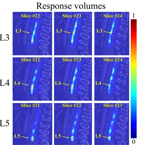
Fig 4. Initial estimation of the VB centers on one test CT image.The estimation is done in a coarse resolution. The response volume of L3, L4, and L5 are visualized in each row, with 3 randomly selected 2D sagittal slices. The diffused probability distribution is observed in the response volumes due to the repetitive pattern of the VBs.
probability:
argmaxc1c
mp1ðc1Þp1;2ðc2jc1Þ pm 1;mðcmjcm 1ÞpmðcmÞ ð6Þ
This can be solved by dynamic programming on the image grids.
2.2 Segmentation of vertebral bodies
The segmentation of VBs is separately done in the defined ROI around each detected VB center
as shown inFig 6. For each voxelvin the defined ROI, we first compute an appearance
likeli-hoodLa(v) (Fig 6, d and e) and a spatial priorPs(v) (Fig 6b and 6c), whereLa(v) is estimated
using the RF soft classification algorithm described below andPs(v) is estimated via a Parzen
window method. In our method, for every voxel in the ROI of a detected VB, we first compute
Fig 5. The fine-tuning step for localization of the estimated VB centers on the same test CT image used inFig 4.The response volume of L3, L4, and L5 are visualized in each row, with 3 randomly selected 2D sagittal slices. The fine-tuning is performed only in a reduced local region around the initial guess obtained from the first step. Thus, the associated probabilities in the response volume are concentrated to a small region.
its spatial priorPs(v). The resultant priorPs(v) serves as a good pre-filter of the potential
fore-ground voxels, where only for those voxels withPs(v)>0.1, we compute its appearance
likeli-hoodLa(v). OncePs(v) andLa(v) are calculated for every voxel, we get the combined posterior
probability mapL(v) (Fig 6d) as:
LðvÞ ¼aPsðvÞ þbLaðvÞ ð7Þ
With the posterior probability mapL(v), for each voxel in the ROI of the VB, its probability of
being the foreground is given. Thefinal binary segmentation is derived by thresholding the
probability map withL(v)0.5 and only keeping the largest connected component. Below we
give the details of using RF soft classification method to estimate the appearance likelihood
La(v).
2.2.1 RF classification based appearance likelihood estimation: Training. Similar to the localization step, given a set of manually labeled training images, we randomly sample a set of 3D training patches {vk= (fk,lk)}k= 1. . .M, wherefkis the visual feature andlk= {1,0} is the fore-ground/background label of the center of a sampled patch, being in the ROI of specified VB.
The sampled training patches can be divided into positive training patches iflk= 1 and negative
training patches iflk= 0. Using both the sampled positive and negative training patches, our
task is then to learn a mapping functionc:Rdf !pðv
kÞ 2 ½0;1from the feature space to the
probability space. We utilize classification forest to train the mapping function. For each forest,
we suppose there areTstrees. Please note we use the same visual feature as we used in the
local-ization step (Sec. 2.1.4).
Fig 6. Segmentation of vertebral body in its ROI.(a): ROI of VB L3. (b)-(e): Segmentation procedure using spatial prior ((b) and (c)) and RF soft
classification based appearance likelihood ((d) and (e)) to estimate the posterior probability (f). The final segmentation results are obtained by a thresholding on the estimated posterior probability.
2.2.2 RF classification based appearance likelihood estimation: prediction. Once the
mapping functionψis learned, for each voxelvin the ROI of a detected VB region, we first
cal-culate its visual featurefv. Through the learned mappingψ, for every voxel in the ROI, we
esti-mate its appearance likelihood of being the foreground/background. Note that each tree in the classification forest will return a predictionpt(lv|fv)2[0, 1], wherelv= {0,1}. Combining all
theseTspredictions allows us to compute a reliable posterior likelihood for each voxelvas
fol-lows.
LaðvÞ ¼pðlvjfvÞ ¼ 1
Ts X
Ts
t
ptðlvjfvÞ ð8Þ
2.3 Implementation details
A Matlab implementation (It is freely available from“http://ijoint.istb.unibe.ch/VB/index.
html”) of the present method is tested using the experiment setup that will be described in Sec.
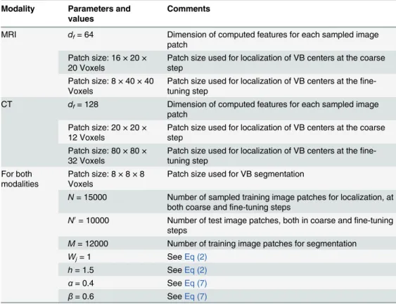
3.1. All parameters used in our experiments are summarized inTable 1. The visual features for
sampled 3D CT/MR image patches are calculated following the description in Sec. 2.1.4. Specif-ically, we evenly divide a sampled patch into 4 × 4 × 4 blocks. Thus for each image patch extracted from a MR image, we compute a 64 dimensional feature and for each image patch extracted from a CT image we compute a 128 dimensional feature.
In the localization stage, for both the coarse detection step and the fine-tuning step we
sam-pleN= 15000 training image patches from training images while for test we sample a set ofN0
Table 1. Parameters used in our experiments.
Modality Parameters and values
Comments
MRI df= 64 Dimension of computed features for each sampled image
patch Patch size: 16 × 20 ×
20 Voxels
Patch size used for localization of VB centers at the coarse step
Patch size: 8 × 40 × 40 Voxels
Patch size used for localization of VB centers at the fine-tuning step
CT df= 128 Dimension of computed features for each sampled image
patch Patch size: 20 × 20 ×
12 Voxels
Patch size used for localization of VB centers at the coarse step
Patch size: 80 × 80 × 32 Voxels
Patch size used for localization of VB centers at the fine-tuning step
For both modalities
Patch size: 8 × 8 × 8 Voxels
Patch size used for VB segmentation
N= 15000 Number of sampled training image patches for localization, at both coarse andfine-tuning steps
N0= 10000 Number of test image patches, both in coarse andfine-tuning
steps
M= 12000 Number of training image patches for segmentation
Wj= 1 SeeEq (2)
h= 1.5 SeeEq (2)
α= 0.4 SeeEq (7)
β= 0.6 SeeEq (7)
the XY plane of the data coordinate system, we choose the patch sizes in different stages as fol-lows. In the localization stage, a patch size of 20 × 20 × 12 voxels is used in the coarse detection step and for the fine-tuning step we use a patch size of 80 × 80 × 32 voxels. For the segmenta-tion stage, we use a patch size of 8 × 8 × 8 voxels.
For both CT and MR images, we empirically choseWj= 1 andh= 1.5 inEq (2),α= 0.4 and
β= 0.6 inEq (7).
3 Experiments and Results
3.1 Experimental design
We validate our method on two openly available CT/MRI datasets: 1) The first dataset contains 23 3D T2-weighted turbo spin echo MR images from 23 patients and the associated ground
truth segmentation. They are freely available from“http://dx.doi.org/10.5281/zenodo.22304”.
Each patient was scanned with 1.5 Tesla MRI scanner of Siemens (Siemens Healthcare, Erlangen, Germany) with following protocol to generate T2-weighted sagittal images: repeti-tion time is 5240 ms and echo time is 101 ms. All the images are sampled to have the same sizes of 39 × 305 × 305 voxels. The voxel spacings of all the images are sampled to be
2 × 1.25 × 1.25 mm3. In each image 7 VBs T11-L5 have been manually identified and
seg-mented, resulting in 161 labeled VBs in total. 2) The second dataset contains 10 3D spine CT
images and the associated ground truth segmentation [21]. They are freely available from
“http://spineweb.digitalimaginggroup.ca/spineweb/index.php?n=Main.Datasets”. The sizes of these CT images are varying from 512 × 512 × 200 to 1024 × 1024 × 323 voxels with intra-slice resolutions between 0.28245 mm and 0.79082 mm and inter-slice distances between 0.725 mm and 1.5284 mm. We further resample all the images into the same voxel spacing of
0.5 × 0.5 × 1.0 mm3, which simplifies the implementation. For each CT image, 5 VBs L1-L5
have been manually annotated, resulting in 50 VBs in total.
Using the two openly available MRI and CT datasets, we evaluated our VB localization and segmentation method with the following 4 experiments:
1. VB localization on MRI dataset. In this experiment, we evaluated the present VB localiza-tion method on the 23 T2-weighted MR images.
2. VB localization on CT dataset. In this experiment, we evaluated the present VB localiza-tion method on the 10 CT images.
3. VB Segmentation on MRI dataset. In this experiment, we evaluated the present VB seg-mentation method on the 23 T2-weighted MR images.
4. VB Segmentation on CT dataset. In this experiment, we evaluated the present VB segmen-tation method on the 10 CT images.
3.2 Evaluation metrics
We propose to use five different metrics to evaluate the performance of the present method, two for localization stage and three for segmentation stage.
For evaluation of the localization performance, we use the following two metrics:
1. Mean localization distance (MLD) with standard deviation (SD)
We first compute the localization distanceRfor each VB center using
R¼
ffiffiffiffiffiffiffiffiffiffiffiffiffiffiffiffiffiffiffiffiffiffiffiffiffiffiffiffiffiffiffiffiffiffiffiffiffiffiffiffiffiffiffiffiffi
ðDxÞ2þ ðDyÞ2þ ðDzÞ2
q
ð9Þ
whereΔxis the absolute difference betweenXaxis of the identified VB center and the VB
center calculated from the ground truth segmentation,Δyis the absolute difference between
Yaxis of the identified VB center and the ground truth VB center, andΔzis the absolute
dif-ference betweenZaxis of the identified VB center and the ground truth VB center.
The equations of MLD and SD are then defined as follows:
MLD¼
PNI
i¼1 PMVB
j¼1 Rij
Nc
and SD¼
ffiffiffiffiffiffiffiffiffiffiffiffiffiffiffiffiffiffiffiffiffiffiffiffiffiffiffiffiffiffiffiffiffiffiffiffiffiffiffiffiffiffiffiffiffiffiffiffiffi PNI
i¼1 PMVB
j¼1 ðRij MLDÞ 2
Nc s
ð10Þ
whereNcis the total number of VBs,NIis the number of patient data, andMVBis the
num-ber of target VBs in each image.
2. Successful detection rate with various ranges of accuracy
If the absolute difference between the localized VB center and the ground truth center is no
greater thantmm, the localization of this VB is considered as a successful detection;
other-wise, it is considered as a false localization. The equation of the successful localization rate
Ptwith accuracy of less thantmm is formulated as follows
Pt¼
number of accurate VB localization
number of VBs ð11Þ
For evaluating the segmentation performance, we use the following three metrics:
1. Dice overlap coefficients (Dice)
This metric measures the percentage of correctly segmented voxels. Dice [38] is computed
by
Dice¼2jA\Bj
jAj þ jBj100% ð12Þ
whereAis the sets of foreground voxels in the ground-truth data andBis the corresponding
sets of foreground voxels in the segmentation result, respectively. Larger Dice metric means better segmentation accuracy.
3. Hausdorff Distance (HSD)This metric measures the Hausdorff distance [39] between the ground truth VB surface and the segmented surface. To compute the HSD, we use the same surface models generated for computing the AAD. Smaller Hausdorff distance means better segmentation accuracy.
3.3 Experimental Results
3.3.1 Localization results on MRI data. Table 2presents MLD with SD when the present method was evaluated on 23 T2-weighted MR images. The localization error (average of the 7 VBs) of each test image as well as overall MLD, SD and median value of all 23 MR images are shown in this table. A localization accuracy of 1.6 ± 0.9 mm was found, which were regarded to be accurate enough for the purpose of defining ROI for each VB region.
Table 3gives the results of successful detection rates of the present method with different
accuracy ranget= 2.0 mm, 4.0 mm, and 6.0 mm, respectively. Given the specified accuracy
ranget= 2.0 mm, our method successfully detected 76.4% VBs. The successful detection rate is
changed to 97.5% when we settto 4.0 mm and all the 161 VBs are successfully detected when
we set accuracy rangetto 6.0 mm.
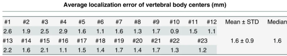
3.3.2 Localization results on CT data. Table 4presents MLD with SD when the present method was evaluated on 10 CT images. The localization error (average of the 5 VBs) of each test image as well as overall MLD, SD and median value are presented in this table. An overall localization accuracy of 1.9 ± 1.5 mm was found, which were regarded to be accurate enough for the purpose of defining ROI for each VB region.
Table 5gives the results of successful detection rates of the present method with different
accuracy ranget= 2.0 mm, 4.0 mm, and 6.0 mm, respectively. Given the specified accuracy
ranget= 2.0 mm, our method successfully detected 58% VBs out of 50 VBs. The successful
detection rate is changed to 94% whentis set to 4.0 mm and this rate is further changed to 96%
when we settto 6.0 mm.
3.3.3. Segmentation results on MRI data. For quantitative evaluation of the present method on the 23 MR images, the Dice, AAD, and HSD between automatic segmentation and
doi:10.1371/journal.pone.0143327.t002
Table 3. Successful detection rate with various ranges of accuracy when evaluated on 23 3D MR images.In the first row, number of successfully detected VBs are given, and in the second row the successful detection rate are shown.
t = 2.0mm t = 4.0mm t = 6.0mm
Number of successfully detected VBs 123 157 161
Successful detection rate (%) 76.4 97.5 100.0
the ground-truth segmentation are calculated over both 3D volumes and 2D mid-sagittal slices. The reason why we also calculate results on 2D mid-sagittal slice is because some of the existing
methods are only evaluated on 2D MR images (e.g., [6,13]).Table 6presents the Dice, AAD,
and HSD (average of the 7 VBs) of each test image as well as overall mean, std and median
val-ues of Dice, AAD, and HSD when calculated on 2D mid-sagittal slice.Table 7presents the
Dice, AAD, and HSD of each image as well as overall mean, std and median values of Dice, AAD, and HSD when calculated on 3D volumes. In summary, we achieved a mean Dice of 92.0 ±3.4%, a mean AAD of 1.0±0.4 mm, and a mean HSD of 4.5±1.4 mm when calculated on 2D mid-sagittal slices. For 3D evaluation, we achieved a mean Dice of 88.7±2.9%, a mean AAD of 1.5±0.2 mm, and a mean HSD of 6.4±1.2 mm.
Table 4. Average localization error (MLD with SD: mm) when evaluated on 10 3D CT data.
Average localization error of vertebral body centers (mm)
#1 #2 #3 #4 #5 #6 #7 #8 #9 #10 Mean±STD Median
1.6 1.9 0.6 1.4 2.5 2.1 2.9 1.4 1.9 2.7 1.9±1.5 1.8
doi:10.1371/journal.pone.0143327.t004
Table 5. Successful detection rate with various ranges of accuracy when evaluated on 10 3D CT images.In the first row, number of successfully detected VBs are given, and in the second row the successful detection rate are shown.
t = 2.0mm t = 4.0mm t = 6.0mm
Number of successfully detected VBs 29 47 48
Successful detection rate (%) 58.0 94.0 96.0
doi:10.1371/journal.pone.0143327.t005
Table 6. Segmentation results when the present method was evaluated on 23 3D MR images with a leave-one-out experiment.The results are calcu-lated on 2D mid-sagittal slices.
Dice overlap coefficient on 2D mid-sagittal slice (%)
#1 #2 #3 #4 #5 #6 #7 #8 #9 #10 #11 #12 Mean±STD Median
89.6 87.7 89.2 86.6 93.6 93.1 91.0 92.9 93.0 92.5 93.6 93.9
#13 #14 #15 #16 #17 #18 #19 #20 #21 #22 #23 92.0±3.4 92.6
93.0 90.9 90.4 93.1 94.9 93.5 92.1 94.4 90.8 92.7 93.2
Average absolute distance on 2D mid-sagittal slice (mm)
#1 #2 #3 #4 #5 #6 #7 #8 #9 #10 #11 #12 Mean±STD Median
1.5 1.4 1.4 1.8 0.8 0.9 1.1 0.8 0.9 0.9 0.8 0.8
#13 #14 #15 #16 #17 #18 #19 #20 #21 #22 #23 1.0±0.4 0.9
0.7 1.2 1.3 0.9 0.6 0.8 0.9 0.7 1.1 1.1 0.8
Hausdorff distance on 2D mid-sagittal slice (mm)
#1 #2 #3 #4 #5 #6 #7 #8 #9 #10 #11 #12 Mean±STD Median
5.9 5.1 6.3 7.6 2.7 3.4 5.6 3.7 3.5 3.5 3.7 4.9
#13 #14 #15 #16 #17 #18 #19 #20 #21 #22 #23 4.5±1.4 4.9
5.5 3.7 6.6 4.2 3.0 3.3 5.1 1.8 5.0 5.5 5.0
InFig 7we visually check the segmentation result of one test MR image on 2D sagittal slices. InFig 8(left part), we compare the segmented surface models of two MR images with the sur-face models generated from the associated ground truth segmentation. It can be clearly seen that the our method achieved good segmentation results on the test MR images when the results obtained with the present method are compared to the corresponding ground-truth segmentation.
3.3.4 Segmentation results on CT data. For quantitative evaluation of the present method on the 10 CT test images, the Dice, AAD, and HSD between automatic segmentation and ground-truth segmentation are calculated over both 3D volumes and 2D mid-sagittal slices. Table 8presents the Dice, AAD, and HSD (average of the 5 VBs) of each test image as well as overall mean, std and median values of Dice, AAD, and HSD when calculated on 2D
mid-sagit-tal slices. Similarly,Table 9presents the Dice, AAD, and HSD of each image as well as overall
mean, std and median values of Dice, AAD, and HSD when calculated on 3D volumes. In sum-mary, we achieved a mean Dice of 90.8±8.7%, a mean AAD of 1.0±0.7 mm, and a mean HSD of 4.3±2.2 mm when evaluated on 2D mid-sagittal slices. For 3D evaluation, we achieved a mean Dice of 91.0±7.0%, a mean AAD of 0.9±0.3 mm and a mean HSD of 7.3±2.2 mm.
InFig 9we visually check the segmentation results of one test CT image on 2D sagittal slices. InFig 8(right part), we compare the segmented surface models of two CT images with the sur-face models generated from the associated ground truth segmentation. It is worth to note that
the second CT data (bottom right image ofFig 8) contains osteophytes in some of the VB
regions. Nevertheless, our method successfully identified and segmented all the 5 VB regions in this CT data with a Dice of 90.7%.
3.3.5 Computation Time. When our Matlab implementation was executed on a computer with 3.0 GHz CPU and 12G RAM, the run-time for the present method could be summarized as follows: 1) For experiments conducted on MR images, on average the run-time of the pres-ent approach to localize and segmpres-ent one image was about 2.0 minutes, in which 0.7 minutes for localization and 1.3 minutes for segmentation. 2) For experiments conducted on CT
Average absolute distance on 3D volume (mm)
#1 #2 #3 #4 #5 #6 #7 #8 #9 #10 #11 #12 Mean±STD Median
1.7 1.6 1.8 1.9 1.5 1.5 1.6 1.6 1.6 1.4 1.4 1.4
#13 #14 #15 #16 #17 #18 #19 #20 #21 #22 #23 1.5±0.2 1.5
1.5 1.6 1.7 1.6 1.3 1.3 1.5 1.3 1.5 1.3 1.3
Hausdorff distance on 3D volume (mm)
#1 #2 #3 #4 #5 #6 #7 #8 #9 #10 #11 #12 Mean±STD Median
6.5 8.3 8.1 8.3 6.7 6.2 7.3 6.2 5.9 5.1 7.8 5.6
#13 #14 #15 #16 #17 #18 #19 #20 #21 #22 #23 6.4±1.2 6.2
6.1 5.5 7.0 6.9 6.1 4.6 7.4 5.0 6.6 4.3 4.7
images, on average the run-time of the present approach to localize and segment one image was about 2.3 minutes, in which 0.5 minutes for localization and 1.8 minutes for segmentation.
The computation time for training RF regressors was respectively about 7.4 minutes for a leave-one-out study conducted on the MR images and 9.7 minutes for a leave-one-out study conducted on the CT images. Although the training phase took relatively longer time when compared to the test phase as described above, we only need to perform the training once in our learning-based method. The trained RF regressors can then be used for any future test image.
4 Discussions
We presented a fully automatic method to localize and segment VBs from CT/MR images. For localization, a RF regression algorithm is used where we aggregate the votes from a set of ran-domly sampled image patches to get a probability map of the center of a target VB in a given image. The resultant probability map is further regularized by HMM to eliminate potential
Fig 7. Segmentation results on one test MR image visualized in 2D sagittal slices.The automatic segmentation (the bottom row) are compared with the ground-truth segmentation (the top row).
Fig 8. Segmentation results visualized with 3D surface models.Images on the left side show the segmentation results on 2 3D MR test images and images on the right side present the segmentation results on 2 3D CT images. It is worth to note that the second CT data (bottom right image) shows osteophytes in some of the VBs but our method successfully identified and segmented all the 5 VB regions in this CT data with a Dice of 90.7%.
doi:10.1371/journal.pone.0143327.g008
Table 8. Segmentation results when the present method was evaluated on 10 3D CT images with a leave-one-out experiment.The results are calcu-lated on 2D mid-sagittal slices.
Dice overlap coefficient on 2D mid-sagittal slice (%)
#1 #2 #3 #4 #5 #6 #7 #8 #9 #10 Mean±STD Median
92.8 88.2 93.6 94.6 88.4 94.1 87.2 95.9 94.6 78.1 90.8±8.7 93.9
Average absolute distance on 2D mid-sagittal slice (mm)
#1 #2 #3 #4 #5 #6 #7 #8 #9 #10 Mean±STD Median
1.0 0.8 0.8 0.7 1.2 0.7 1.9 0.6 0.9 1.5 1.0±0.7 0.8
Hausdorff distance on 2D mid-sagittal slice (mm)
#1 #2 #3 #4 #5 #6 #7 #8 #9 #10 Mean±STD Median
3.4 4.2 3.2 3.6 7.5 4.0 3.5 2.2 2.0 9.0 4.3±2.2 3.6
Table 9. Segmentation results when the present method was evaluated on 10 3D CT images with a leave-one-out experiment.The results are calcu-lated on 3D volumes.
Dice overlap coefficient on 3D volume (%)
#1 #2 #3 #4 #5 #6 #7 #8 #9 #10 Mean±STD Median
91.8 90.7 93.4 93.8 87.0 92.6 90.1 94.5 93.8 82.0 91.0±7.0 93.0
Average absolute distance on 3D volume (mm)
#1 #2 #3 #4 #5 #6 #7 #8 #9 #10 Mean±STD Median
1.0 0.8 0.7 0.8 1.1 0.7 1.3 0.7 0.9 1.0 0.9±0.3 0.8
Hausdorff distance on 3D volume (mm)
#1 #2 #3 #4 #5 #6 #7 #8 #9 #10 Mean±STD Median
5.0 7.3 7.7 6.0 10.3 5.5 10.0 5.8 5.3 10.2 7.3±2.2 6.6
doi:10.1371/journal.pone.0143327.t009
Fig 9. Segmentation results on one test CT image visualized in 2D sagittal slices.The automatic segmentation (the bottom row) are compared with the ground-truth segmentation (the top row).
accurate results on both MR and CT images.
Compared with the user-supplied methods [3,6,7], the present method can achieve VB
localization fully automatically without any user-intervention. The automatic strategy has the advantages of reducing measurement time and improving clinical study quality. Our experi-mental results demonstrated the efficiency and accuracy of the RF regression based method with: 1) average localization time about 0.7 minute for detecting 7 VB regions from a 3D MR image and 0.5 minute for detecting 5 VB regions from a 3D CT image, and 2) a mean localiza-tion error of 1.6 mm when evaluated on MR images and 1.9 mm when evaluated on CT images.
To the best of our knowledge, this is the first time to apply RF classification for VB segmen-tation in CT/MR images. Although there exist works using RF classification for medical image
segmentation, they are only specified to segment soft tissues like kidney in CT images [30].
Furthermore, our experimental results demonstrated the accuracy and robustness of the RF classification based method for VB segmentation in CT/MR images. More specifically, the present method achieved a mean Dice of 88.7% when evaluated on 3D MR images and a mean dice of 92.0% when evaluated on 2D mid-sagittal MR slices. In comparison with GT based methods for MR image segmentation, the present method achieved better results. For example,
the 2D square-cut method [6] achieved an average Dice of 90.97% while the 3D cube-cut
method [20] achieved an average Dice of 81.33%. Nevertheless, due to the fact that different
datasets are used in evaluation of different methods, direct comparison of different methods is difficult and should be interpreted cautiously.
Most of the work [4,5,16,21,40] on spine CT image processing focuses on segmentation
and there are a few studies addressing automatic localization of vertebrae in CT scan [8,17,
40]. Random forest regression was used in both [8] and this study for an automatic localization
of vertebrae from CT scans but with different visual feature design. In comparison with the
results reported in [8] where an average localization error of 6.06 mm was reported for lumbar
vertebrae, our method achieved better results, with an average localization error of 1.9 mm. Again, due to different datasets used in evaluation of different methods, such a comparison
should be interpreted cautiously. It is worth to note that the datasets used in [8] are much
more diverse than the CT datasets used in our study, which may pose a challenge to their method and partially explain why we have achieved better results. In comparison with other spine CT segmentation methods, the CT segmentation accuracy of the present method is
slightly worse than those model-based approaches [4,5,21], though the present method
achieves a segmentation accuracy on 3D MR images that is comparable to the state-of-the-art
spine MRI segmentation methods [3,6,15,20]. For example, evaluated on the same datasets,
the method introduced in [21] achieved an average Dice coefficient of 93.6% while the
5 Conclusions
In summary, this work has the research highlights as described below:
1. Proposed a fully automatic, unified RF regression and classification framework;
2. Solved the two important problems of localization and segmentation of VB regions from a 3D CT image or a MR image with the unified framework;
3. Validated and evaluated the proposed framework on 10 3D CT data and 23 3D MRI data;
4. Achieved comparable or equivalent segmentation performance to the state-of-the-art methods.
Acknowledgments
This work was partially supported by the Swiss National Science Foundation with Project No. 205321_157207/1.
Author Contributions
Conceived and designed the experiments: GZ. Performed the experiments: CC. Analyzed the data: CC GZ. Contributed reagents/materials/analysis tools: CC GZ. Wrote the paper: CC GZ DF DLB MB GA. MR image data acquisition: DF DLB MB GA.
References
1. Freburger JK, Holmes GM, Agans RP, Jackman AM, Darter JD, Wallace AS, et al. The Rising Preva-lence of Chronic Low Back Pain. Archives of Internal Medicine. 2009; 169(3):251–258. doi:10.1001/
archinternmed.2008.543PMID:19204216
2. Miao J, Wang S, Wan Z, Park W, Xia Q, Wood K, et al. Motion Characteristics of the Vertebral Seg-ments with Lumbar Degenerative Spondylolisthesis in Elderly Patients. Eur Spine J. 2013; 22(2):425–
431. doi:10.1007/s00586-012-2428-3PMID:22892705
3. ZukićD, Vlasak´ A, Dukatz T, Egger J, Horinek D, Nimsky C, et al. Segmentation of Vertebral Bodies in MR Images. In: Goesele M, Grosch T, Preim B, Theisel H, Toennies K, editors. Proceeding of 17th International Workshop on VMV; 2012. p. 135–142.
4. Aslan MS, Ali A, Farag AA, Rara H, Arnold B, Xiang P. 3D Vertebral Body Segmentation Using Shape Based Graph Cuts. In: Pattern Recognition (ICPR) 2010. Istanbul; 2010. p. 3951–3954.
5. Ali AM, Aslan MS, Farag AA. Vertebral body segmentation with prior shape constraints for accurate {BMD} measurements. Computerized Medical Imaging and Graphics. 2014;38(7):586–595. Special
Issue on Computational Methods and Clinical Applications for Spine Imaging. Available from:http:// www.sciencedirect.com/science/article/pii/S0895611114000603
6. Egger J, Kapur T, Dukatz T, Kolodziej M, ZukićD, Freisleben B, et al. Square-Cut: A Segmentation Algorithm on the Basis of a Rectangle Shape. Plos One. 2012; 7(2). doi:10.1371/journal.pone. 0031064
7. Ayed B, Puni K, Minhas R, Joshi KR, Garvin GJ. Vertebral body segmentation in MRI via convex relaxa-tion and distriburelaxa-tion matching. In: Ayache N, Delingette H, Golland P, Mori K, editors. Medical Image Computing and Computer-Assisted Intervention—MICCAI 2012. vol. 7510 of LNCS. Springer Berlin
Heidelberg; 2012. p. 520–527.
8. Glocker B, Feulner J, Criminisi A, Haynor DR, Konukoglu E. Automatic Localization and Identification of Vertebra in Arbitrary and Field-of-view CT Scans. In: Ayache N, Delingette H, Golland P, Mori K, edi-tors. Medical Image Computing and Computer-Assisted Intervention—MICCAI 2012. vol. 7512 of
LNCS. Springer Berlin Heidelberg; 2012. p. 590–598. Glocker2012
9. Schmidt S, Kappes J, Bergtholdt M, Pekar V, Dries S, Bystrov D, et al. Spine detection and labeling using a parts-based graphical model. In: Karssemeijer N, Lelieveldt B, editors. Proceeding of IPMI 2007. vol. 4584 of LNCS. Kerkrade, The Netherlands: Springer Berlin Heidelberg; 2007. p. 122–133.
–
doi:10.1109/TMI.2009.2023362PMID:19783497
14. Carballido-Gamio J, Belongie SJ, Majumdar S. Normalized Cuts in 3-D for Spinal MRI Segmentation. IEEE Transactions on Medical Imaging. 2004; 23(1):36–44. doi:10.1109/TMI.2003.819929PMID:
14719685
15. ZukićD, Vlasak´ A, Egger J, Horinek D, Nimsky C, Kolb A. Robust Detection and Segmentation for Diagnosis of Vertebral Diseases Using Routine MR Images. Computer Graphics Forum. 2014; 33 (6):190–204. doi:10.1111/cgf.12343
16. Klinder T, Wolz R, Lorenz C, Franz A, Ostermann J. Spine Segmentation using Articulated Shape Mod-els. In: Metaxas D, Axel L, Fichtinger G, Szekely G, editors. Medical Image Computing and Computer-Assisted Intervention—MICCAI 2008. vol. 5241 of LNCS. New York, USA: Springer H; 2008. p. 227–
234.
17. Klinder T, Ostermann J, an A Franz ME, Kneser R, Lorenz C. Automated Model-based Vertebra Detec-tion, IdentificaDetec-tion, and Segmentation in CT image. Medical Image Analysis. 2009; 13(3):471–482. doi:
10.1016/j.media.2009.02.004PMID:19285910
18. Štern D, Likar B, Pernus F, Vrtovec T. Parametric Modelling and Segmentation of Vertebral Bodies in
3D CT and MR Spine Images. Phys Med Biol. 2011; 56:7505–7522. doi:10.1088/0031-9155/56/23/
011PMID:22080628
19. Yao J, OConnor SD, Summers RM. Automated Spinal Column Extraction and Partitioning. In: Proceed-ing of 3rd IEEE International Symposium on Biomedical ImagProceed-ing: Nano to Macro. ArlProceed-ington, VA: IEEE; 2006. p. 390–393.
20. Schwarzenberg R, Freisleben B, Nimsky C, Egger J. Cube-Cut: Vertebral Body Segmentation in MRI-Data through Cubic-Shaped Divergences. PLOS ONE. 2014; 9(4). doi:10.1371/journal.pone.0093389 PMID:24705281
21. Ibragimov B, Likar B, PERNUS F, Vrtovec T. Shape Representation for Efficient Landmark-Based Seg-mentation in 3-D. Medical Imaging, IEEE Transactions on. 2014 April; 33(4):861–874. doi:10.1109/
TMI.2013.2296976
22. Breiman L. Random forests. Machine Learning. 2001; 45(1):5–32. doi:10.1023/A:1010933404324
23. Criminisi A, Shotton J, Robertson D, Konukoglu E. Regression Forests for Efficient Anatomy Detection and Localization in CT Studies. In: Menze B, Langs G, Tu Z, Criminisi A, editors. Proceedings of MIC-CAI 2010 Workshop MCV. vol. 6533. Berlin, Heidelberg: Springer-Verlag; 2010. p. 106–117.
24. Chen C, Belavy D, Zheng G. 3D Intervertebral Disc Localization and Segmentation from MR Images by Data-driven Regression and Classification. In: Wu G, Zhang D, Zhou L, editors. MLMI 2014. vol. 8679 of LNCS. Springer Switzerland; 2014. p. 50–58.
25. Kolmogorov V, Zabih R. What energy functions can be minimized via graph cuts? IEEE Trans Pattern Anal Mach Intell. 2004; 26(2):147–159. doi:10.1109/TPAMI.2004.1262177PMID:15376891
26. Boykov Y, Kolmogorov V. An Experimental Comparison of Min-Cut/Max-Flow Algorithms for Energy Minimization in Vision. IEEE Trans Pattern Anal Mach Intell. 2004; 26(9):1124–1137. doi:10.1109/
TPAMI.2004.60PMID:15742889
27. Li K, Wu X, Chen DZ, Sonka M. Optimal surface segmentation in volumetric images-A graph-theoretic approach. IEEE Trans Pattern Anal Mach Intell. 2006; 28(1):119–134. doi:10.1109/TPAMI.2006.19
PMID:16402624
28. Song Q, Bai J, Garvin MK, Sonka M, Buatti JM, Wu X. Optimal Multiple Surface Segmentation With Shape and Context Priors. IEEE Trans Med Imag. 2013; 32(2):376–386. doi:10.1109/TMI.2012.
2227120
29. Lindner C, Thiagarajah S, Wilkinson JM, arcOGEN Consortium, Wallis G, Cootes TF. Fully Automatic Segmentation of the Proximal Femur using Random Forest Regression Voting. IEEE Trans Med Imag. 2013; 32(8):1462–1472. doi:10.1109/TMI.2013.2258030
editors. Medical Image Computing and Computer-Assisted Intervention—MICCAI 2012. vol. 7512 of
LNCS. Springer Berlin Heidelberg; 2012. p. 66–74.
31. Yang C, Duraiswami R, Davis L. Efficient Kernel Machines Using the Improved Fast Gauss Transform. Advances in neural information processing systems. 2005; 17:1561–1568.
32. Chu C, Chen C, Liu L, Zheng G. FACTS: Fully Automatic CT Segmentation of a Hip Joint. Annals of Biomed Eng. 2015; 43(5):1247–1259. doi:10.1007/s10439-014-1176-4
33. Jaeger F, Hornegger J. Nonrigid Registration of Joint Histograms for Intensity Standardization in Mag-netic Resonance Imaging. IEEE Trans Med Imaging. 2009; 28(1):137–150. doi:10.1109/TMI.2008.
2004429
34. Li C, Gore JC, Davatzikos C. Multiplicative intrinsic component optimization (MICO) for MRI bias field estimation and tissue segmentation. Magnetic Resonance Imaging. 2014; 32(7):913–923. doi:10.
1016/j.mri.2014.03.010PMID:24928302
35. Tustison NJ, Avants BB, Cook PA, Zheng Y, Egan A, Yushkevich PA, et al. N4ITK: Improved N3 Bias Correction. IEEE Trans Med Imaging. 2010; 29(6):1310–1320. doi:10.1109/TMI.2010.2046908PMID:
20378467
36. Jaeger F. Normalization of magnetic resonance images and its application to the diagnosis of the scoli-otic spine. Logos Verlag Berlin GmbH; 2011.
37. P Viola P, Jones M. Rapid object detection using a boosted cascade of simple features. In: CVPR 2001. vol. I; 2001. p. 511–518.
38. Dice LR. Measures of the Amount of Ecologic Association Between Species. Ecology. 1945; 26 (3):297–302. doi:10.2307/1932409
39. Huttenlocher DP, Klanderman GA, Rucklidge WJ. Comparing images using the Hausdorff distance. Pattern Analysis and Machine Intelligence, IEEE Transactions on. 1993 Sep; 15(9):850–863. doi:10.
1109/34.232073