i
SPATIO-TEMPORAL ANALYSES OF THE RELATIONSHIP BETWEEN
ARMED CONFLICT AND CLIMATE CHANGE IN THE EASTERN AFRICA
Riazuddin Kawsar
ii
SPATIO-TEMPORAL ANALYSES OF THE RELATIONSHIP BETWEEN ARMED CONFLICT AND CLIMATE CHANGE IN THE EASTERN AFRICA
Supervisor:
Prof. Dr. Edzer J. Pebesma. Institute for Geoinformatics (IFGI), Westfälische Wilhelms-Universität (WWU),
Münster, Germany.
Co-supervirors:
Prof. Dr. Jorge Mateu M Department of Mathematics,
Universitat Jaume I (UJI) Castellon, Spain.
&
Prof. Mário Caetano
Instituto Superior de Estatística e Gestão de Informação (ISEGI) Universidade Nova de Lisboa (UNL),
Lisbon, Portugal. February 2011
&
Prof. Dr. Pedro Cabral
Instituto Superior de Estatística e Gestão de Informação (ISEGI) Universidade Nova de Lisboa (UNL),
Lisbon, Portugal.
iii
Dedication
iv
Acknowledgments
I am very grateful to my supervisor Edzer Pebesma, co-supervisors Professor Jorge Mateu for taking time off a busy schedule to supervise me at every stage of this project. Thanks to my co-supervisors Professor Mário Caetano and Professor Pedro Cabral of ISEGI-UNL, Lisbon for the face-lifting comments on the manuscript.
I am most grateful to the European Commission for, through the Erasmus Mundus scholarship scheme, making my studies and stay as comfortable as they were during these eighteen months. Thanks to the staff of the three partner universities - Institute for Geoinformatics Muenster, Universitat Jaume I, Castellon Spain and New University of Lisbon Portugal for ensuring a smooth run of the entire program.
I am indebted to the Research Groups Photogrammetry & Remote Sensing, Department of Geodesy and Geoinformation, Vienna University of Technology, especially Richard Kidd for allowing me to use data (Surface Soil Moisture) collected by the project. I also thank to Uppsala Conflict Data Program‟s (UCDP) for the Armed conflict dataset.
I am also grateful to Professor Pablo Juan Verdoy of UJI, Spain for helping me with R software.
Many thanks to my classmates who made the period of my studies an interesting ride. I sincerely thank my family and friends for supporting me and for giving me the vote when I decided to take up this Master program. Their prayers and support were invaluable.
Above all, I am thankful to God Almighty for His amazing grace. At every point of the work, I really felt my prayers answered.
v
Declaration of Originality
I declare that the submitted work is entirely my own and not belongs to any other person. All references, including citation of published and unpublished sources have been appropriately acknowledged in the work. I further declare that the work has not been submitted to any institution for assessment for any other purpose.
Münster, 28th February 2013
vi
SPATIO-TEMPORAL ANALYSIS OF THE RELATIONSHIP BETWEEN ARMED CONFLICT AND CLIMATE CHANGE IN THE EASTERN AFRICA
Abstract
vii
Keywords
o Armed Conflict
o Climate Change
o Spatial Point Pattern analysis
o Spatial distribution pattern
o Spatio-temporal modelling
o Spatial Autoregressive model
o Climate conflict relationship
viii
Acronyms
o AC - Armed Conflict
o AI - Area Interaction
o AIC - Akaike‟s Information Criterion
o CC - Climate Change
o CIESN - Center for International Earth Science Information Network
o CSR - Complete Spatial Randomness
o ERS - European Remote Sensing
o GDP - gross domestic product
o GED - Geo-referenced Event Dataset
o GPW - Gridded Population of the World
o ICP - Inhomogeneous Cluster Process
o ICTP - Inhomogeneous Cluster Thomas Process
o IMCP - Inhomogeneous Matern Cluster Process
o IPCC - Intergovernmental Panel on Climate Change
o IPP - Inhomogeneous Poission Process
o OLS - Ordinary Least Square
o PPP - Point Pattern Process
o SAG - Space Advisory Group
o SAR - Spatial Autoregressive Model
o SCM - Spatial Cluster Process model
o SDM - Spatial Durbin Model
o SEM - The Spatial Error Model
o SPI - Standerized Precipitation Index
o SSA - Sub Saharan Africa
o SSM - Surface Soil Moisture
o STIKhat - Space-time inhomogeneous K-function
o SWI - Soil Water Index
o UCDP - Uppsala Conflict Data Program
ix
Table of content
1 Chapter 1: Background ... 1
1.1 Armed conflict ... 1
1.2 Climate change ... 1
1.3 Armed conflict and climate change ... 2
1.4 Why this study? ... 4
1.5 Data in such study ... 5
1.6 Study area ... 6
1.7 Methods used to support the climate conflict relationship ... 7
1.8 Research questions ... 8
1.9 Research design ... 9
1.10 Research writing organization... 9
2 Chapter 2: Methodology and Data ... 11
2.1 Methodology ... 11
2.2 Point process analyses ... 11
2.3 Lattice approach ... 12
2.4 Data ... 13
2.4.1 Sources and dataset construction ... 13
2.5 Descriptive statistics ... 18
3 Chapter 3: Armed Conflict and Point Process Modelling ... 21
3.1 Intensity ... 22
3.1.1 Dependence of intensity on a covariate... 23
3.2 Test for Complete Spatial Randomness ... 24
3.3 Inhomogeneous poisson process ... 25
3.3.1 Model I: Inhomogeneous poisson process ... 25
3.3.2 Intensity estimation for inhomogeneous poisson process. ... 26
3.3.3 Inhomogeneous K-function ... 27
3.3.4 Interpretation of Kinhom with Linhom-function ... 28
3.3.5 Model fitting and simulation ... 29
3.4 Model II: Inhomogeneous poisson cluster process ... 30
3.4.1 Modelling procedure: ... 31
x
3.5 Gibbs mode model IV: area-interaction process ... 34
3.5.1 Model fitting and simulation: ... 35
3.6 Yearly plot of K function ... 37
3.7 Space time point process modelling ... 40
3.7.1 Estimation of the space-time inhomogeneous K-function ... 40
4 Chapter 4: Lattice Approach ... 45
4.1 Spatial cross-sectional models ... 45
4.1.1 Spatial autoregressive model (SAR) ... 45
4.1.2 The spatial error model (SEM) ... 45
4.1.3 Spatial durbin model (SDM): ... 46
4.2 Spatial cross-sectional modeling: ... 47
4.3 Impacts in Spatial Lag models ... 48
4.4 Spatio-temporal lattice approach modeling: ... 50
5 Chapter 5: Discussion and Conclusion ... 53
5.1 Point process models ... 54
5.1.1 Spatial point process model fitting and selection ... 54
5.1.2 Spatio-temporal point process modeling ... 56
5.2 Lattice approach ... 57
5.2.1 Spatial regression models ... 58
5.2.2 Spatio-temporal regression models ... 59
5.2.3 Climate change and armed conflict ... 60
5.3 Conclusion ... 61
6 Referances ... 63
7 ANNEX 1(yearly K-function plot) ... 70
xi
List of figures
Figure 1-1 the distribution of the Armed Conflict in Africa ... 7
Figure 2-1 space time plot of Soil Water Index (SWI) ... 15
Figure 2-2 spatial time series of annualized Weighted Anomaly Weighted Anomaly Standardized soil water index (WASWI) ... 17
Figure 2-3 spatial time series of annualized Standardized precipitation index (SPI) ... 18
Figure 2-4 season pattern of armed conflict in the study region. ... 19
Figure 2-5 standardized trend plot of Armed Conflict and WASWI ... 20
Figure 2-6 regression line of AC and WASWI ... 20
Figure 3-1 Quadrat count of Event data ... 22
Figure 3-2 Perspective plot of event density ... 22
Figure 3-3 Events Intensity as a functions of Spatial Covariate population ... 23
Figure 3-4 Events Intensity as a functions of Spatial Covariate WASWI ... 23
Figure 3-5 Events Intensity as a functions of two Spatial Covariate SPI and WASWI ... 24
Figure 3-6 Events Intensity as a functions of two Spatial Covariate population and WASWI ... 24
Figure 3-7 Spatial Kolmogorov-Smirnov test of CSR with population ... 25
Figure 3-8 Spatial Kolmogorov-Smirnov test of CSR with SPI ... 25
Figure 3-9 Spatial Kolmogorov-Smirnov test of CSR with WASWI ... 25
Figure 3-10 Estimation of the inhomogeneous intensity surface ... 29
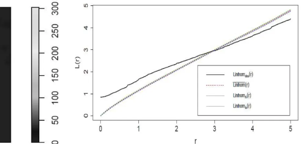
Figure 3-11 estimate of inhomogeneous K-function (right and black solid line) for the crime data sets. ... 29
Figure 3-12 Point-wise critical envelopes for inhomogeneous version of the L-function in Inhomogeneous Matern Process; ; the data line (black), theoretical line (red) ... 33
Figure 3-13 Thomas Process, obtained from 99 simulations where the Upper envelope is point-wise maximum of simulated curves and Lower envelope is point-wise minimum of simulated curves; the data line (black), theoretical line (red) ... 33
Figure 3-14 Profile log pseudolikelihood values for the Trend formula: Armed Conflict ~population+ WASWI + SPI; fitted with rbord= 4; Interaction: Area Interaction with irregular parameter „r‟ in [100, 200 km]. Optimum value of irregular parameter: r = 100 km ... 36
Figure 3-15 : Pointwise critical envelopes for inhomogeneous version of the L-function in Inhomogeneous Area Interaction Process, obtained from 99 simulations of fitted Gibbs model where the Upper envelope is point-wise maximum of simulated curves and Lower envelope is point-wise minimum of simulated curves; Significance level of Monte Carlo test: 2/100 = 0.02‟ Data: Inhomogeneous Area Interaction with fitted parameter „r‟ in [100 km]; Trend formula: Armed Conflict ~population+ WASWI+SPI ... 36
Figure 3-16 Inhomogeneous Thomas cluster process for the year 1999 (with covariates of the year 1999) ... 38
xii
Figure 3-18 Inhomogeneous Thomas cluster process for the year 1999 (with covariates of the
year 1997) ... 38
Figure 3-19 Inhomogeneous Matern cluster process for the year 1999 (with covariates of the year 1999) ... 38
Figure 3-20 Inhomogeneous Matern cluster process for the year 1999 (with covariates of the year 1999) ... 38
Figure 3-21 Inhomogeneous Matern cluster process for the year 1999 (with covariates of the year 1999) ... 38
Figure 3-22 Inhomogeneous Matern cluster process for the year 1997 (with covariates of the year 1997) ... 38
Figure 3-23 Inhomogeneous Matern cluster process for the year 1997 (with covariates of the year 1996) ... 38
Figure 3-24 Inhomogeneous Matern cluster process for the year 1997 (with covariates of the year 1995) ... 38
Figure 3-25 Year wise fitted coefficients of WASWI with different temporal lag ... 39
Figure 3-26 Year wise fitted coefficients of SPI with different temporal lag ... 39
Figure 3-27 Year wise fitted coefficient of Population with different temporal lag ... 40
Figure 3-28 Image of the spatial intensity based on kernel... 42
Figure 3-29 Image of the spatial intensity based on covariates ... 42
Figure 3-30 with small u (up to 440 km) and v (up to 20 days) for the case events without covariates ... 43
Figure 3-31 with small u (up to 440 km) and larger v (up to 2 years app.) for the case events without covariates ... 43
Figure 3-32 with larger u (up to 1500 km) and v (up to 2 years app.) for the case events without covariates ... 43
Figure 3-33 with small u (up to 440 km) and v (up to 20 days) for the case events with covariates ... 43
Figure 3-34 with small u (up to 440 km) and larger v (up to 2 years app.) for the case events with covariates ... 43
Figure 3-35 with larger u (up to 1500 km) and v (up to 2 years app.) for the case events with covariates ... 43
Figure 3-36 Superimposed events (red) with simulated (black) rpp using karnel (1st cases) . 43 Figure 3-37 Superimposed events (red) with simulated (black) rpp using karnel (2nd cases) 43 Figure 3-38 Superimposed events (red) with simulated (black) rpp using Covariates (1st cases) ... 44
Figure 3-39 Superimposed events (red) with simulated (black) rpp using Covariates (2nd cases) ... 44
Figure 3-40 P-value for STIKhat with small u (up to 440 km) and v (up to 20 days) for the case events without covariates from 100 simulations ... 44
Figure 3-41 P-value STIKhat for small u (up to 440 km) and larger v (up to 2 years app.) for the case events without covariates from 100 simulations ... 44
xiii
Figure 3-43 P-value for STIKhat with small u (up to 440 km) and v (up to 20 days) for the case events with covariates from 100 simulations ... 44 Figure 3-44 P-value STIKhat for small u (up to 440 km) and larger v (up to 2 years app.) for the case events with covariates from 100 simulations ... 44 Figure 3-45 P-value for STIKhat with larger u (up to 1500 km) and v (up to 2 years app.) for the case events with covariates from 100 simulations ... 44 Figure 4-1 Neighbors addressed for of temporally lagged SAR model (left), mode 2 (middle) and model 3 (right). This figure is adapted from Espindola, Pebesma, et al. (2011). ... 51 Figure 5-1 Standardized fitted coefficients for Inhomogeneous cluster point process models ... 56
List of tables
Table 2-1 Descriptive statistics of Armed Conflict, weight) Anomaly Standardized soil water index (WASWI ) and Standardized Precipitation Index (SPI) ... 19 Table 3-1 Fitted coefficients for trend formula: ~population + WASWI + SPI ... 33 Table 3-2 Fitted coefficients for trend formula Armed Conflict ~population+ Weighted Anomaly Standardized soil water index + Standardized Precipitation Index using
1
1
Chapter 1: Background
1.1 Armed conflict
Armed conflict can be termed as a conflict between or among several parties which involves armed forces. In 2001 Wallenstein and Sollenberg redefined the definition
of armed conflict. According to them, “an armed conflict is a contested incompatibility which concerns government and/or territory where the use of armed force between two parties, of which at least one is the government of a state, results in at least 25 battle-related deaths.” Armed conflict can be categorized into several categories based on their magnitude, involving parties, duration of conflict etc. but Uppsala Conflict Data Program (UCDP) categories the organized violence into three major categories in their dataset, Geo-referenced Event Dataset (GED). (Strandow et al. 2011). The categories are (1) state-based armed conflict, (2) non-state conflict and (3) one-sided violence. UCDP had compiled and coded information of organized
violence‟s in event form for all three conflict types, covering the entire time period
1989-2010 for the African continent. The dataset defines armed conflict or events as,
“…The incidence of the use of armed force by an organized actor against other organized actor, or against civilians, resulting in at least 1 direct death in either the best, low or high estimate categories at a specific location and for a specific temporal
duration” (Strandow et al. 2011). Each event was appended with additional information like the date, scale, perpetrator etc. Different types of events differ in the aspects such as duration, temporal precision and continuity in armed violence. From 1989 to 2010, they have recorded around 22,000 events. For this study we have only considered all kinds of continuous violence for the period 1991 to 2000, which includes 3289 events in our study area in the Eastern African continent (see Figure 1.1 in page no 10).
1.2 Climate change
The temperature increase is not only warming the world but also deciding the fate of human being associated with the implications of warming the earth's surface. So global climate change became a very popular topic in the international research community. Impact of climate change is now evident and water is at the heart of it.
2
security literature, we can find that the access to the natural resources is a major predictor of armed conflict (Homer- Dixon 1991, 1999; Kahl 2006). Study on long term trend in temperature and precipitation change in light of human security can revile the notion. Understanding the impact of climate change on human security can lead us towards better conflict prediction by reconciling climate change and environmental security in the same ground.
Global warming is likely to affect the water availability pattern by affecting the precipitation pattern and that is pushing us to the ground of unpredictability of extreme events and this kind of situation may have implications for peace and security. So, understanding the climate change and its effect on life, cold be a very important study topic.
1.3 Armed conflict and climate change
Scarcity of resources such as minerals and water and conflict over that scarce resource is an old source of armed conflict. Resource scarcity will be intensified by environmental degradation and therefore will contribute to an increase in armed conflict (Gleditsch et al. 2011). Different authors argued otherwise on this topic. Fearon and Laitin (2003) argue that the probability of conflict can be increased by poverty since poor states have a much weaker financial and bureaucratic basis, providing an opportunity for riot. Besides poverty, low economic growth and high dependence on primary commodity exports are also important predictors of civil war. Then again, ethnic and religious diversity as well as democracy may not affect the risk of war (Collier and Hoeffler 2004). On the other hand, Hegre et al. 2001 found that regime type and ethnic heterogeneity matter have a greater impact on development. So, most of the studies on armed conflict have identified several economic, social, demographic or political factors as the main indicators of armed conflict until recently. In the first quantitative study of environmental conflict, Hauge et al. 1998 have found that economic and political factors were the strongest predictors of conflict but that environmental and demographic factors did have some impacts too. The world is generally becoming more peaceful but the debate on climate change presents the climate change as a potential threat to a new source of instability and conflict (Gleditsch et al. 2011).
3
Several studies have found the potential link between climate change and armed conflict. Different authors argued that climate change is not the only factor of armed conflict but it may make the situation more tense coupled with some other economic, social or political factors. For example, Gleditsch et al., 2011 argued that reduced rainfall and higher temperature that jointly causes droughts and that reduces the access to the natural capital what sustains livelihoods. As a result, existing poverty will be more widespread and this kind of property situation and crisis are potential sources for a greater conflict.
Some more recent studies of temperature variation and conflict (Burke et al., 2009, 2010) claimed to find a link between temperature and civil war in Sub-Saharan Africa for the period 1981–2002 and argued that over a 35- year period climate change has contributed to a major increase in the incidence and severity of civil war in the region. Then again, Bernauer et al., 2012 have applied the temperature and precipitation deviations as a function of economic growth and thereafter have seen that, these variations in climate variables can predict onset of civil conflict in a non-democratic settings. Miguel et al. (2004) also has argued that anomalies of rainfall can be considered as another factor for armed conflict because he has found a relationship between negative rainfall deviation and increased risk of civil war in Africa. Again Miguel (2005) has found that both positive and negative extremes in rainfall increased the frequency of conflicts and has killed a lot of people in a rural
Tanzanian district. On the other hand, D‟Exelle and Campenhout (2010) have found water scarcity to drive conflicting behavior, particularly so for poor and marginalized households. Several statistical studies of conflict in Africa have found social violence and communal conflict to be most likely in or following wet periods (Raleigh and Kniveton 2012; Theisen 2012). The extreme events of natural disaster are another implication of climate change and one study using survey material on Indonesia finds villages that had suffered a natural disaster during the preceding three years to be more likely to experience violent conflict (Barron et al. 2009). Then again, sea-level rise, which is another implication of climate change, will threaten the livelihood of the populations of small island states in the Indian Ocean, the Caribbean, and the Pacific. Studies that look at non-random sets of cases with out-migration in areas with severe environmental degradation provide suggestive evidence that climate change could trigger more human mobility and that is also a source of conflict (Reuveny 2007; Reuveny and Moore 2009).
4
armed conflict for better understanding which may lead the modeler to a more accurate conflict scenario simulation.
One of the major criticisms of the early environmental security literatures are, those studies tended to neglect important political and economic context factors (Gleditsch 1998), but they are connected to each other. This study is also an attempt at the reconciliation of environmental with limited socioeconomic factors to draw a more justifiable conclusion.
1.4 Why this study?
Economical and political factors are very important for the armed conflict study (Fearon and Laitin 2003). In several studies it‟s been observed that Poverty increases the likelihood of the war and climate change is putting further pressure on the significance of the poverty level. So, several researchers are considering climate change as a factor or economic growth reduction and negative economic growth as a factor of armed conflict. On the other hand, in some other studies it‟s been evidenced that when we control the income, ethnic and religious diversity it does not increase the risk of conflict (Collier and Hoeffler 2004). Last few years, the researchers found a new dimension to observe the armed conflict linking climate change and its effect perspective but most of the researches are suffering from different kind of deficient. For an instance, the Case-based Environmental Security literature contains several narratives of violent conflict within the context of resource competition and environmental degradation but suffers from proper methods. Some of these quantitative researches found a potential scarcity-conflict connection but suffer from poor data and inappropriate research designs. There are some potential researches identified above give some indication that climate change increase risk of armed conflict but there are disagreements too. Another limitation of the previous studies can be identified as Incompatibilities of scale as several studies are conducted which focuses on countries not on subnational level, whether it‟s been pointed that most of the armed conflict cases are a local phenomenon. Besides, spatial statistics wings provide us extraordinary tools and methods to model the relationship between armed conflict armed conflict climate change from spatial time series analysis but almost no spatial time series analysis has been done in such study or suffers from poor data and inappropriate research designs. So it can be concluded that there are still no concrete solutions, which give modellers an idea how to incorporate climate change in armed conflict modeling or the question is still unanswered, how good climate change indicators would be to predict armed conflict?
5
tomorrow‟s word peace today. Modelling the relationship between armed conflict
and climate change for future scenario prediction can be the start point of the nexus to clime walk towards peace by taking a right decision for the particular space and particular time. This study has tried to fill some of the identified research gaps in the study arena of climate change and armed conflict.
1.5 Data in such study
This study is mainly concentrated on finding the potential link between climate change and armed conflict for better understanding of the complex human environment interaction in the light of armed conflict. By modelling the relationship between armed conflict and climate change we can derive the mathematical link, which might help the researcher to predict the dynamic of armed conflict which are induced by the change in climate.
The instability of a country is the indicator of potential armed conflict which depends on some explanatory independent variable and their link with the risk on the armed conflict. To measure the instability of a country the explanatory variables used in several researches in this arena are basically some structural facts which can be identified as Economic indicators (gross domestic product (GDP) and its growth rate), Socio-demographic (total population, population density, youth bulge, school enrolment, infant mortality rate, ethnic polarization, regional polarization), Resources and their distribution ( inequality: GINI Index, natural resource: ratio between primary commodity exports and GDP), Geographical context (Proximity and nature of the border, Terrain characteristics), Regime (level of democracy), Development Indicators (export, import, investment, foreign debt etc.), Climate change factors (precipitation, temperature, sea level rise and extreme disaster events), History of armed conflict ( armed conflict event and location) etc. (Burnley et al. 2008).
6
have found that soil moisture depends on the climate change indicator precipitation, temperature, evaporation etc. and can cause extreme events such as draught (for detail about WASWI preparation see the Data section). For an instance Lakshmi et al. (2003) has molded the relationship between the surface temperature and soil moisture and showed that increase of temperature corresponds to a decrease in the soil moisture. So soil moisture level can depict the temperature scenario for a particular region. Then again Xu et al. (2012) have shown the relationship between soil water and rainfall. So, WASWI can be a good indicator of rainfall and temperature though there are other factors related to soil water containment such as soil type. Again, some study provides a clear picture about the relationship between climate change, soil moisture and agricultural production such as Tao et al. (2003) and which corresponds to our study area characteristics and so WASWI is a better explanatory climate variable for the study area like Sub Saharan Africa (SSA). So this WASWI can be considered as a good indicator of climate change as studies have identified SWI as an indicator of climate change already (Seneviratne et al. 2010). WASWI can offer a better picture of climate change as it a factor which not only consider precipitation or temperature alone but also the interplay of these factors. Besides WASWI we also have incorporated other climate change indicators which are good for draught study and already used in climate conflict study (Theisen et al. 2010) is Standardized Precipitation Index (SPI), which is considered as a well-known probabilistic measure of the severity of a dry event (Guttman 1999) and that explains the physical and climatic situation of our study area well (Collier et al. 2008).
1.6 Study area
Almost every country has experienced armed conflict in several locations and in different time periods. To get a more accurate picture it is recommended to do such study on the whole world with a large range of explanatory variables. But due to time, resource and data limitations we needed to consider a small portion of the SSA for this study. Choosing a study region was tricky and again easy enough. It was tricky because a small portion is not enough to draw a relationship between conflict and climate for the whole world as the space is continuous and heterogeneous in characteristics both in the physical and socioeconomic sense. And it was easy to
decide because of available data sets. In several literatures it‟s been termed that Sub Saharan Africa (SSA) is the place on earth which experienced most of armed conflict events and therefore potential for such study. Then again being in the lower latitude the climate change effect will be more moderate than most other locations. So we decided to choose the Eastern part of Sub Saharan Africa as our study area.
7
economies as this continent is one of the largest agricultural sectors of the world. Global warming is likely to lead to a drying of most of the Africa. It is generally accepted that Africa will be affected by future global climate change first and most severely. (Low 2005; Collier et al. 2008).
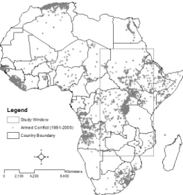
From the figure 01 we can see that most of the armed conflict event over the time period 1991 to 2000 are distributed in the eastern part of the Africa. Then again the study window in Blue boundary can be characterized as a diversified area because of its geographical feature distribution (e.g., water body, dry region, central African forest etc.) as well as heterogeneous distribution of armed conflict (e.g., zone experienced Armed Conflict and zone without experiencing armed conflict).
Figure 1-1 the distribution of the Armed Conflict in Africa (Strandow et al. 2011)
The total land area of Africa continent is approximately 29063244 sq.km and our study window is about 8719926 sq.km which means more than 30 percent area are covered by our study window. Then again based of the UCDP armed conflict dataset named geo-referenced Event Dataset (GED), over the period 1991 to 2000 the African Continent experienced around 10708 numbers of armed conflict of what 3289 numbers of armed conflict are inside the study window. Because of the characteristics, the number of conflict event distribution and efficiency of analysis, we have considered the blue banded box as our study window.
1.7 Methods used to support the climate conflict relationship
8
models (Theisen et al. 2010). Some other have adopted linear regression with country fixed effects and time trends (Buhaug 2010). There some other studies too which involved some other method besides logistic regression. For an example Raleigh and Kniveton (2012) has used Negative binomial count regression and composite analysis (or „epoch superposition‟) methodology and Miguel et al. (2004) has used a nonparametric version of the local regression method with an Epanechnikov kernel etc.
Continuous development in probability wing Point Process modeling has provided us with more sound techniques to model and predict point process (e.g., event data can be considered as a point process according to the definition of point process. For detail see chapter 3). For an instance Zammi -Mangion et al. (2012) while studying the dynamic of war in Afghanistan has involved dynamic spatio-temporal modelling from point process theory. Until now that was the first involvement of point process theory in the Armed Conflict study but only to model the war dynamics no to study the climate conflict relationship. In our study we tried to model armed conflict (events) and climate change related information from spatial patterns of events; insights from point process theory. We have used five models in several phases. Poisson Process model, Thomas Cluster Model, Matern Cluster Model, Area Interaction Model for both spatial and spatio-temporal process. Space-time inhomogeneous K-function (STIKhat) has been used to assess the dynamic spatio-temporal point process modelling. Besides point process modeling we have also considered lattice approach and have completed some spatial regressive models like Ordinary Least Square (OLS) model, Spatial Autoregressive (SAR) model, Spatial Error Model (SEM) and Spatial Durbin Model (SDM). Then again we have computed spatio temporal models devising SAR model for spatial, temporal and spatio-temporal neighbors.
1.8 Research questions
1. Is there any link between climate change and conflict?
2. Is local resource scarcity (e.g., soil moisture) in terms of climate change offers a better prediction of conflict behavior?
3. Is the climate problem may arise and persist locally?
4. May sub national disaggregated studies provide more support for the resource conflict nexus?
5. If there is any link between climate change and armed conflict, then how good climate change indicators are predicting armed conflict?
9
analyses. Here is our basic assumptions were the distribution of conflict location are inhomogeneous due to the varying distribution of climatic factors. For an instance, areas with lower levels of water contained in soil and higher number of population are more prone to conflict.
1.9 Research design
Ambition: modeling the relationship between armed conflict and climate change and analysis of the central environmental security proposition that Climate Change increases the local risk of civil armed conflict
Sample: Eastern region of Sub Saharan Africa (SSA) 1991 – 2000 (10 years)
Unit of analysis
o Spatial: 0.5 degree latitude x 0.5 degree longitude grid cell observations. In this part of the world each side of the cells corresponds to approximately 55 kilometers
o Temporal: year
Dependent variable: Geo-referenced armed conflict occurrences which have >25 battle‐deaths threshold.
Independent Variable
o Weighted Anomaly Soil Water Index (WASWI)
o Soil Water Index (SWI)
o Standardized Precipitation Index (SPI)
o Number of Population etc.
Method
o Different models of point process theory
o Different models from lattice approach
1.10 Research writing organization
This report is organized in 6 major sections with several subsections, which follow a chronological flow of ideas as follows
In the background (chapter 1) section we have talked about the relationship between climate change and armed conflict form environmental security literature and also talked about the previous study attempts, their limitations, about the data and methods used in such study etc. we have also included our research question and research design in chapter 1.
10
The point process modeling (chapter 3) explains the point process models used in this study to understand the interaction and covariate effect on the conflict distribution and also presents detail modeling approach and results of the point process models.
The lattice approach (chapter 4) explains the spatial and spatio-temporal lattice approach modeling and their result.
11
2
Chapter 2: Methodology and Data
2.1 Methodology
To model the relationship between armed conflict and climate change, our first step was to decide the list of covariates and independent variables, which can explain the relationship between our independent variable and covariates. As this was a spatio-temporal study, we also had to put some extra attention on choosing the covariates because of data unavailability for different time period and extent of our study area.
It was also important to choose a particular spatial area for the study based on data availability for different spatial and temporal period. It was also a major concern about the size of the area for efficient computation, due to time limitation. For our study, based on the data available and efficient processing and computing capability we have chosen the eastern part of the African continent.
In the next step we have constructed a dataset which has the structure of a raster grid. Our unit of observations is subnational “cells” of 0.5 degrees of latitude x 0.5 degree of longitude. All the data were being processed according to that particular resolution.
Our empirical analysis was conducted in the cell and cell by year level. In this study our main dependent variable is events, an integrated measure of conflict indicating the total number of any kind of conflict (have >25 battle‐deaths threshold) indicating whether the cell has experienced a conflict related episode of any of the categories included in the UCDP GED dataset over the period of the year 10 years from 1991 to 2000. And our covariates were the number of the total population per cell, The Standardized precipitation Index (SPI) per cell and Weighted Anomaly Standardized soil water index (WASWI) per cell etc.
In order to investigate the local level relationship between climate change and the armed conflict incidence we have estimated several models from point process theory and from lattice approach.
2.2 Point process analyses
From point process theories we have estimated four models for spatial patterns of events analysis and to estimate the covariate effects on event distribution.
12
(ITCP) and Inhomogeneous Matern Cluster Process (IMCP). And our final model for point process is an Area Interaction (AI) model which not only considers the covarite effect but also inter point interaction to define an intensity function for point distribution in a study area (for detail see chapter 3). For this entire model we have used the inhomogeneous version of K-Function (for detail chapter 3) to fit our empirical data with theoretical lines of different models.
The behaviors of a point process can be explained through trend (caovariate effect) and dependence (interaction) between the points of a point pattern. The appearance of such interaction or trend consists of either clustering or regularity in the process. A widely used tool for exploring the nature of interaction is a Ripley‟s K-function (Ripley 1976; Diggle 2003; Cressie 1993). In our study we use an Inhomogeneous version of L-Function to interpret an Inhomogeneous version of K-Function.
In the first part of the point process modelling, we have excluded the temporal dimension of all of the data by aggregating all data into one spatial layer. So, resulting models are based on aggregated event data for the period 1991-2000 as main dependent variable and aggregated WASWI, SPI and number of population as covariates.
In the second part of the study we have fitted all of these four kinds of model with empirical yearly data for 10 years (1991-2000) which explains the relationship between armed conflict and climate by year. while mdelling, besides yearly covariates we have also considered covariates of different temporal lag such as (t-1) and (t-2)
In the third part of the study the Second-order properties are used to analyze the spatio-temporal structure of a point process. The space-time inhomogeneous K-function are used as a measure of spatio-temporal clustering or regularity and as a measure of spatio-temporal interaction (Gabriel and Diggle 2009; Moller and Ghorbani 2012, Illian et al. 2008).
2.3 Lattice approach
13
Simultaneous Autoregressive Lag model (SAR) analyses by considering autocorrelation of the dependent variables in space which was done by using a spatial weight matrix (e.g., considered queen neighbors) (model 1.2). We have also incorporated two other models from Spatial Autoregressive model wing. Those are The Spatial Error Model (SEM); termed as model 1.3, Spatial Durbin Model (SDM); termed as model 1.4 (for detail see chapter 4, spatial modelling section).
In the next step of the lattice approach we have integrated the temporal dimension into the analysis by defiing the spatial, temporal and spatio-temporal neighbors in SAR model (for detail, see chapter 4 spatio-temporal modelling section). We have modified the SAR model for temporal neighbors which has given us one single autocorrelation coefficient to define the correlation both in space and time; we have termed this as model 2. We have also devised the model 2 to fit another single correlation coefficient to describe correlations between all (spatial, temporal, and spatio-temporal) neighbors. For all these models we have also calculated the Nagelkerke R-squared to understand the impact of covariates on our dependent variable, Armed Conflict.
2.4 Data
2.4.1 Sources and dataset construction
For this study we bring together georeferanced data from a variety of sources and constructed a dataset which cover almost 16 countries either partially or completely. The study area consists of the eastern part of Central African Republic, Sudan, Zaire, Eastern part of Angola (app. 25 %), Zambia, northern part of Zimbabwe ( app. 75 %), northern part of Mozambique (app. 75 %), Malawi, Tanzania, Burundi, Rwanda, Uganda, Kenya, western part of Ethiopia (app. 60 %), western part of Eritrea (app. 75 %) and a small portion of Botswana. The data set contains the information of every location (cell) over the period 1991-2000, which includes the information of individual conflict episode locations. We have also collected, computed and processed the detailed data on SWI, WASWI, SPI and the number of population. All these data are processed according to 0.5 degree latitude x 0.5 degree longitude degree raster grid.
2.4.1.1 Armed conflict
According to the event definition in Sundberg et al. 2010, Uppsala Conflict Data
one-14
sided violence. This data set is the most disaggregated datasets which indicated the location with 10 meter accuracy. In this dataset, the number of deaths at the event location, start time and end time of the event, these kinds of attributes are attributed against the event location. For such local level study this dataset is being used in different study (Melander et al. 2011) and was able to explain the nature of conflict in SSA.
In our study data on armed conflict episodes over the period 1991-2000 are collected from comprehensive version 1.5 of Geo-referenced Event Dataset (GED) dataset developed by UCDP. In our study area, we have considered all kinds of conflicts recorded in GED datasets. The number of total events is 3289 where the total number of state-based armed conflict is 1558, 299 non-state conflict and 1432 one-sided violence. For computational effectiveness we have spread the overlapped points up to 50 meters for aggregated point pattern analysis and for lattice process analyses that was not necessary as the data were prepared in cell level based on event count.
2.4.1.2 Weighted anomaly standardized soil water index
Surface Soil Moisture (SSM): The Surface Soil Moisture (SSM) data from Research Groups Photogrammetry & Remote Sensing, Department of Geodesy and Geoinformation, Vienna University of Technology (TUWIEN). SSM is a time series of the topsoil which indicates a relative measure of the water content in the surface layer (<5 cm from the surface) ranging between 0 and 1. SSM data were derived from scatterometers on-board in the The European Remote-sensing Satellites (ERS-1 and ERS-2) by considering microwave frequencies 1-10 GHz domain as the dielectric properties of soil and water are distinctly different in these frequencies (Pradhan and Saunders 2011). The collected data resolution is like following
Spatial Resolution 50 sq.km
Temporal Resolution = daily
The IPCC Fourth Assessment Report states, European Environment Agency and so others also have proved and consider that Soil moisture is an important factor that influences the climate (Weaveret and Avissar 2001; Gregory et al. 1997; Boix-Fayos et al. 1998; Komescu et al. 1998)
15
pushed harder in the years ahead. So here TUWINE comes with a solution by the computing Soil Water Index (SWI).
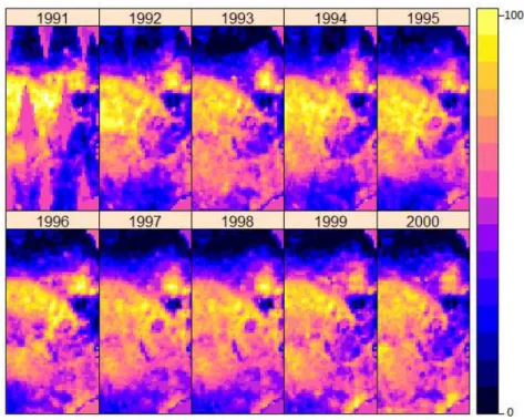
Soil Water Index (SWI): The retrieved SSM, being a topsoil signature, may change significantly within a few hours whose magnitude depends on the amount of rainfall, evaporation rate and the time lapse since the rainfall event. The Soil Water Index (SWI) for the top 1 meter layer thus estimated from the topsoil moisture content adjusted with precipitation, evaporation etc. (Pradhan et al. 2011). So, the retrieved information is generally in good agreement with general climate regimes and gridded precipitation data. (Scipal, 2002). SWI is generally in good agreement with general climate factors like Precipitation, temperature, evaporation and has been used in Several climate change Studies. For an instance for use of SWI for drought indices in climate change impact assessment (Mavromatis 2010), soil moisture datasets for unravelling climate change impacts on water resources (Wagner et al. 2011), water cycle changes and CMIP3 simulations (Mariotti et al. 2008), monitoring water availability and precipitation distribution at three different scales (Zhao et al. 2007) etc. A plot of yearly SWI is shown in figure 2-1, where the 0 value represents relatively (the value is spatially relative) dry region.
Figure 2-1 space time plot of Soil Water Index (SWI)
16
within the framework of the Global Monitoring for Environment and Security (GMES) project geoland2 aims to minimize this gap.
SWI data from January 1st 2007 until the end of 2010 were compared to in situ soil moisture data from 420 stations belonging to 22 observation networks which are available through the International Soil Moisture Network. These stations delivered 1331 station/depth combinations which were compared to the SWI values. After excluding observations made during freezing conditions the average significant correlation coefficients were 0.564 (min -0.684, max 0.955) while being greater than 0.3 for 88% of all stations/depth combinations (Albergel et.al. 2009 and 2012; Parrens et.al. 2012).
WASWI estimation: Suppose 𝑊𝐴𝑆𝑊𝐼 is the Weighted Anomaly Weighted Anomaly Standardized soil water index which represents a dimensionless measure of the relative severity of the Soil Water Index (SWI) surplus or deficit in a grid cell x
and according to (Lyon and Barnston 2005) that can be defined as:
𝑊𝐴𝑆𝑊𝐼 = ∑ ( ̅̅̅̅̅̅ ) ̅̅̅̅̅̅̅ ̅̅̅̅̅̅ ……… (1)
Where 𝑠𝑤𝑖 = is the observed value of SWI for the ith month;
𝑠𝑤𝑖
̅̅̅̅̅̅ = represent long term (1991-2000) mean of monthly SWI for the ith
month;
𝜎 = standard deviation of the anomalies of monthly SWI for the ith month;
𝑠𝑤𝑖
̅̅̅̅̅̅ = mean annual SWI and
̅̅̅̅̅̅
̅̅̅̅̅̅̅ = Weighting factor representing the monthly fraction of annual SWI to
reduce large standardized SWI anomalies that might result from small precipitation amounts or higher temperature and evaporation, occurring near the start or end of dry seasons and to emphasize anomalies during the heart of rainy seasons.
For our study, according to equation (1) we have calculated the WASWI for the month January like following
𝑊𝐴𝑆𝑊𝐼 = ( 𝑠𝑤𝑖 𝑠𝑤𝑖̅̅̅̅̅̅̅̅̅̅̅̅̅̅̅̅̅̅̅̅̅̅̅̅̅̅̅̅̅̅̅̅̅̅̅̅ 𝜎
)
𝑠𝑤𝑖
̅̅̅̅̅̅̅̅̅̅̅̅̅̅̅̅̅̅̅̅̅̅̅̅̅̅̅̅̅̅̅̅̅̅̅̅ 𝑠𝑤𝑖
̅̅̅̅̅̅̅̅̅̅̅̅̅̅̅̅̅̅̅̅̅̅̅̅̅̅̅̅̅̅̅̅̅̅̅
17
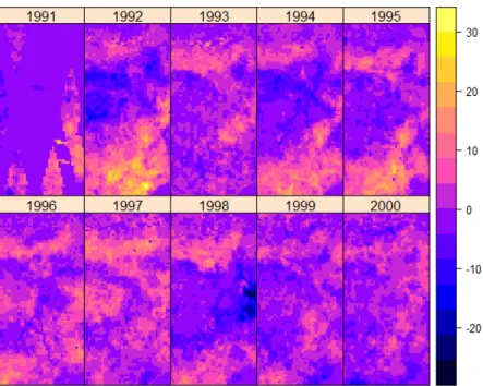
respectively. From the plot we can observe that in 1992, 1994 and 1998 some region of our study area have experienced relatively extreme dry condition.
Figure 2-2 spatial time series of annualized Weighted Anomaly Weighted Anomaly Standardized soil water index (WASWI)
2.4.1.3 Standardized precipitation index
The Standardized Precipitation Index (SPI) is a probability index which has been developed by McKee et al. (1993 and 1995) to give a better depiction of irregular wetness and dryness than the conventional Palmer indices (Palmer 1965). The index is standardized by transforming into the probability of the observed precipitation, which enables all users to have a common basis for both spatial and temporal comparison of index values. SPI is a probability based invariant indicator of drought that recognizes the importance of time scales in the analysis of water availability and water use (Guttman 1999).
To calculate SPI first a probability density function which describes the long term time series of observed precipitation. In our case the series is for 1 year time duration. In the next step the cumulative probability of an observed precipitation amount is computed. Then by applying the inverse normal (Gaussian) function, with mean zero and variance one to the cumulative probability we can get the SPI for 1 year time duration. SPI values can be positive or negative where the magnitude of the departure from zero in negative direction considered as a probabilistic measure of the severity of a dry event.
18
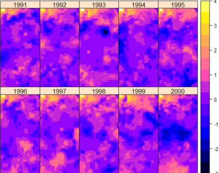
downloaded for the whole world from this site. http://iridl.ldeo.columbia.edu/ SOURCES/.IRI/.Analyses/.SPI/.dataset_documentation.html. To make the data compatible with our annual armed conflict data, we converted the monthly SPI index into an annual index. A plot of annualized SPI is shown in figure 2-2, where negative values and positive values indicate the unusually dry and unusually wet condition, respectively.
Figure 2-3 spatial time series of annualized Standardized precipitation index (SPI)
2.4.1.4 Population
Center for International Earth Science Information Network (CIESIN) has developed the datasets titled Gridded Population of the World (GPW), which is a collection of subnational administrative boundary data and corresponding population estimates for the world. The data set covers twenty year period, from the late 1980s to the present. The first version of GPW was based on 19,000 subnational units and version three incorporates more than 350,000 subnational units, each with georeferenced boundaries and at least one corresponding population estimate (Balk et al. 2003). The spatial resolutions of the data sets are 2.5 minutes latitude by 2.5 minutes longitude, which is approximately 21 sq. km at the equator. For our study purpose we have collected the data for available years for our study period (1991, 1995 and 2000) regrided the data into 0.5 degree latitude x 0.5 degree longitude grid.
2.5 Descriptive statistics
19
season there might appear an economic shock due to decrease in agricultural productive. By instinct we assumed that there might be some pattern in armed conflict which might be derived from the hampered agricultural growth. To understand this phenomenon we tried to look for some seasonal pattern in our study area for the period 1991 to 2000. From the plot 2-4 we can see that there were no seasonal pattern in armed conflict in the study area but we have observed the increase in the number of armed conflicts in that period (1991-2000). So we have decided to go with the yearly study then the seasonal study.
Figure 2-4 season pattern of armed conflict in the study region.
We have divided the whole study area into 3200 sub-region (cells of 0.5 degree longitude x 0.5lattitude). Table 2-1 presents the descriptive statistics of both dependent and independent variables in the study of cells. From the table we can observe that the mean armed conflict was higher in 1996 and 2000 and standard deviation also follows the trend. On the other hand WASWI was highest in 1995
Table 2-1 Descriptive statistics of Armed Conflict, weight) Anomaly Standardized soil water index (WASWI ) and Standardized Precipitation Index (SPI)
Year AC (Mean)
AC (SD)
WASWI (Mean)
WASWI (SD)
SPI (mean)
SPI (SD)
1991 0.08 0.59 3.37 5.85 0.12 0.68
1992 0.06 0.47 2.99 7.95 0.18 0.66
1993 0.08 0.67 1.32 3.59 0.33 0.79
1994 0.12 1.73 1.46 5.77 0.08 0.76
1995 0.08 1.00 5.79 2.52 0.18 0.84
1996 0.20 1.91 4.18 2.74 0.28 0.67
1997 0.20 1.45 3.57 4.18 0.41 0.71
1998 0.24 1.66 -0.41 5.80 0.33 0.74
1999 0.19 1.51 0.30 3.66 0.27 0.81
2000 0.22 1.86 0.35 3.41 0.02 0.96
Total 1.48 12.84 22.91 45.46 2.21 7.60
0 50 100 150
1 5 9 1 5 9 1 5 9 1 5 9 1 5 9 1 5 9 1 5 9 1 5 9 1 5 9 1 5 9
1991 1992 1993 1994 1995 1996 1997 1998 1999 2000
20
(SWI anomaly in a positive direction, means relatively more water in the soil but anomaly was higher as well) and in 1998 (SWI anomaly negative direction, means less water in the soil). The lowest mean value of SPI was observed in 2000 and highest in 1997.
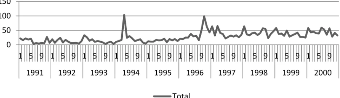
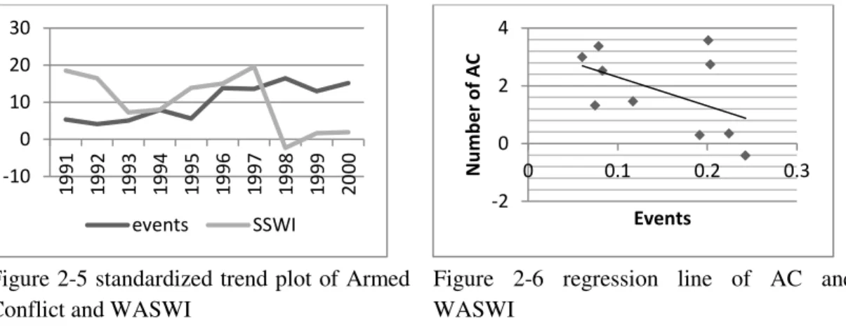
Figure 2-5 standardized trend plot of Armed Conflict and WASWI
Figure 2-6 regression line of AC and WASWI
Following the aim of our study we have considered WASWI as our main independent variable which considered as a climate change indicator and armed conflict as the dependent variable. We have plotted regression line in figure 2-5 and 2-6. From the figures we can see that the events and WASWI have a negative relationship. In the period 1991 to 1994 the value of WASWI decreased and the
number of armed conflicts increased. But in 1995 it‟s the contrary. Then again the
first statement is also true for the period 1998 to 2000. So the relationship doesn‟t follow a linear trend. We have also plotted the regression line between these two variables in figure 2-6. There we can observe the negative relationship more clearly and the relationship can be expressed through y = -9.9635x + 3.2927 where R² = 0.2508. -10 0 10 20 30 19 91 19 92 19 93 19 94 19 95 19 96 19 97 19 98 19 99 20 00 events SSWI -2 0 2 4
0 0.1 0.2 0.3
21
3
Chapter 3: Armed Conflict and Point Process Modelling
A point process “...a stochastic process in which we observe the locations of some events of interest within a bounded region A.” (Bivand et al. 2007). In the definition the events refer to the actual observations of points, while the region A is usually considered as the window of observation (Baddeley and Turner 2006). In another word, a point process is a collection of random points in a n-dimensional space falling in any bounded set, where for spatial point process n =2 and for spatio-temporal case n =3 (Ripley 1952). According to the definition of point process, the location of armed conflicts is realized as a set of random points in a 2-dimensional space (spatial point process case) falling in our study window and 3-dimensional space for spatio-temporal point process case. Location (e.g., longitude and latitude of an event) of armed conflict can be characterized by a broad range of heterogeneous explanatory variables such as geographical, political and socioeconomic variables in several formats (spatial, non-spatial or spatio-temporal). And these make the modelling and prediction of conflict challenging due to heterogeneous and dynamic nature of the data available.
In this section, the goal of armed conflict location study based on point process theory to identify and understand the complex underlying process in conflict such as interaction, diffusion, heterogeneous growth and hotspot of armed conflict based on the location properties of covariates and interaction between the conflict events. Such study of conflict dynamics, insights from point process theory can provide a predictive framework which helps us to understand the dynamic process of conflict based on the dependence between points and covariates and it can also provide the level of confidence in terms of prediction. In this section, we have studied the spatial or spatio-temporal dependence between points, spreading phenomenon and transformation and covariates effect on event‟s distributions with statistical accuracy.
As the basic point process is a Poisson process (Ripley 1977), the starting point of any point process study is the homogeneous Poisson process or Complete Spatial Randomness (CSR) (Schabenberger and Gotway 2005), where the intensity in even across the study space. If the intensity does vary spatially then the process is referred to the inhomogeneous Poisson process.
22
expected value of a point process (e.g., Poisson process). The empirical nearest neighborhood function (G-Function) explains the probability of an observed nearest neighborhood of a point appearing at any given distance, which describes the degree of clustering of regularity in any point process. There are several summary functions used in point process studies but all these summary functions (e.g., G-Function, F-functions) considers only the nearest neighbor for each event in a process which can be identified as major drawback but K-Functions are based on all the distances between events in a study region. So, as suggested in several studies, in our study we fit our point process model with the data with K-Function (Ripley 1977)
Simulation process lies in the heart of the point process study. After a model fitted to the data the simulation can be done and based on the simulation we can create the simulation envelops which is the basic tool to estimate the confidence in modelling and prediction (Schabenberger and Gotway 2005). In this study, the term event represents an armed conflict episode and point of sets refers to an arbitrary location
3.1 Intensity
One of the basic properties of point process modeling is intensity. Exploring intensity which also can be termed as the average density of points, we can estimate the expected number of points per unit. Then again, intensity may be homogeneous or inhomogeneous. In the first step of analysis we have investigated the intensity of events. In the study region the event intensity is 4.11 means the expected number of events in each 100 sq. km is 4.11. To check the homogeneity or inhomogeneity we have conducted Quadret Count Test and we have found that the intensity is not homogeneous (see Figure 3-1 and 3-2).
23 3.1.1 Dependence of intensity on a covariate
To explore the dependence of event intensity on covariates we have estimated the relative distribution of events as a function of different covariates. Let us assume that the intensity of the conflcit point process is a function of the covariate Z (Population, WASWI and SPI). Let, Z(u) be the value of the covariate then at any spatial location
u, the intensity of the point process will be
= ( )
Where ρ is a function which explains how the intensity of AC depends on the value of the covariates. In our case, we have used Kernel smoothing to estimate the function ρ, using methods of relative distribution or relative risk, as explained in Baddeley and Turner (2006)
In the figures 3-3 and 3-4 the plots are some estimate of the intensity ρ(z) as a function of different covariates. It indicates that the events are relatively unlikely to be found where the number of the population is low or less than 1000 (see figure 3-3) on the other hand events are likely to be found where the WASWI value is low or dry region (maximum number of events are likely to be found in the range of -1 to -2). This Relative distribution estimate gives a signal that the intensity of the events depends on the values of a covariate. In both cases the pper and lower limit were of pointwise 95% confidence interval.
Figure 3-3 Events Intensity as a functions of Spatial Covariate population
Figure 3-4 Events Intensity as a functions of Spatial Covariate WASWI
24
both cases for SPI and WASWI, it is most likely that the events are most likely to be found where the values of covariates are relatively low on the other hand the events are most likely to be found where the number of population is high and values of WASWI is low (see figure 3-6).
3.2 Test for Complete Spatial Randomness
The basic benchmark model of a random point pattern is the uniform Poisson point process with homogeneous intensity λ, can be termed as Complete Spatial Randomness (CSR). If the point pattern is completely random then the points are completely unpredictable and have no trend. In our study our null model was a homogeneous poison process. If our null model is true then our points are independent of each other and have the same propensity to be found at any location. To find the evidence against CSR one of the classical tests of the null hypothesis of CSR is Chi-squared test of CSR using quadrat counts. So, we have estimated the Chi-squared test and the p-value was less than 0.001. Inspecting the p-value, we see that the test rejects the null hypothesis of CSR for the event data. As there are so many criticisms of chi-squared test in classical literature (see Baddeley and Turner 2005) in the next step we have conducted Kolmogorov-Smirnov test of CSR, where we have used population, WASWI and SPI as spatial covariates. The test output has been plotted in figure 3-7,3-8 and 3-9. In the plot we can see that the test reject our null model of CSR for the event data. So we continued our study of the Inhomogeneous point process.
Figure 3-5 Events Intensity as a functions of two Spatial Covariate SPI and WASWI
25 Figure 3-7 Spatial
Kolmogorov-Smirnov test of CSR with population
Figure 3-8 Spatial Kolmogorov-Smirnov test of CSR with SPI
Figure 3-9 Spatial Kolmogorov-Smirnov test of CSR with WASWI
3.3 Inhomogeneous poisson process
The rejection of the null hypothesis for Complete Spatial Randomness (CSR) leads to have a closer look with more fine-grained analysis of point processes. So as suggested in Schabenberger and Gotway (2005) we have constructed our second hypothesis that maybe Inhomogeneous Poisson processes lead to clustering of events because we have observed that the intensity varies spatially (Figure 3-2).
More fine-grained analysis was led by four models. The first model has been chosen for the events data set is an Inhomogeneous Poisson process, the second is an inhomogeneous Thomas process, third one is an inhomogeneous Matern Cluster process and another one model which is considered in this study for our data sets is inhomogeneous (non-stationary) Area Interaction Point Process model.
3.3.1 Model I: Inhomogeneous poisson process
The ihomogeneous Poisson process of intensity λ > 0 has some particular properties. Such as under CSR the expected number of points falling in any region A is
[ 𝐴 ] = 𝐴 and n points which can be represented as 𝐴 are independent and uniformly distributed in window A but in inhomogeneous Poisson process the intensity function λ(u) are replaced by inhomogeneous intensity function. So now the number of point n falling in a region A has expectation
[ 𝐴 ] = ∫
where u is a particular location in region A. Then again, n points are independent and have unequal success probability density
26
The inhomogeneous Poisson process is a credible model for point patterns under several scenarios. One is random thinning. Under such scenario the probability of expecting a point at the location is . Then the resulting process of expecting points is inhomogeneous Poisson, with intensity = .
Inhomogeneous Poisson processes generate often clustered patterns. An area in the observed window, where intensity is high, obtains a greater density of events than the area where intensity is low. So an inhomogeneous Poisson process is sensitive to be selected as a model for our study where event intensity varies spatially (Diggle 2003).In our study a model of events expectation in a particular location, which assumes that all events are independent of each other, with an outbreak probability that depends on the local climate conditions like WASWI or number of Population. The resulting pattern of events is an inhomogeneous Poisson process.
3.3.2 Intensity estimation for inhomogeneous poisson process.
The estimate of intensity λ(u) at the location u is denoted by ̂(u) and it is calculated by estimation of density at the location u. Suppose x is a set of a point pattern where
= { } in a compact window 𝐴 then the density estimator function
f(x) at x0 (which isdefined as the number of samples within distance d from x0) is
defined to be
̂ = ∑ ( )
where k(s) is the uniform density on-1 ≤ s ≤1
Estimation of f(x0) is unbiased for a small neighborhood d but, it suffers from large
variability. To minimize the large variability we have used Gaussian kernel instead of uniform kernel function, which does not refer to equal weight for all points inside the region x0 ± d, and that is defined to be
𝑠 =
√ ( 𝑠
)
The probability estimate of an event at u location can be estimated from density estimation and the density estimation can integrate to one over the region A. The intensity and the density in region A are related as
27
= ∫
The product of two univariate kernel functions finds a kernel function product for a process in . Suppose the co-ordinates of x are yi and zi, the intensity estimator is
defined by the product-kernel functions (Schabenberger and Gotway 2005) as follows:
̂ = 𝐴 ∑ ( )
( )
where dy and dz are the bandwidths in the respective directions of the co-ordinate
system. The edge corrected kernel intensity estimator with a single bandwidth is given by
̂ = ∑ ( )
Where = ∫ ( )
is played the role as the edge correction.
3.3.3 Inhomogeneous K-function
The k-function known as Reply‟s K-function or reduced second moment function of a stationary point process x is defined to estimate the expected number of additional random points within a distance r of a random point x1, which was first introduced by
Ripley (1977). λK(r) equals to the expected number of random points within a distance r of x1 where lambda is the intensity of the process and K(r) = πr2
Deviations between the theoretical and empirical K curves may suggest spatial clustering or spatial regularity( Diggle 1983).
Ripley's K function is defined only for stationary point processes. A modification of the K-function can be used in inhomogeneous processes to the aggregation in events which was proposed by Baddeley et al. (2000). In inhomogeneous Poisson processes, events are independent in the subregion, but the intensity λ(x) varies spatially throughout the region
The inhomogeneous K function Kinhom(r) is a direct generalization to non-stationary
28
=
where is a function and which is defined by the spatial lag and the interaction between the arbitrary events x and y. So, the product of the first-order intensities at x and y multiplied by a spatial correlation factor refers to the second-order intensity of the inhomogeneous Poisson processes. If the spatial interaction between the points of the process at the location x and y is 0 then =
as = . And if ||.|| is the Euclidean norm then the pair correlation function is defined as
(|| ||) =
The corresponding intensity reweighted K-function is
= ∫
For an inhomogeneous Poisson process where there is no spatial interaction between events then the inhomogeneous K-function is = as for the homogeneous case. In the spatstat package the standard estimators of K-function can be extended to the inhomogeneous K-function (Baddeley et al., 2000) as below
̂ = 𝐴 ∑ ∑𝑤 𝐼
̂ ̂
where 𝐴 is an area of the study region, denote distance between the ith and jth
observed points and
and 𝑤 is an edge-correction weight and ̂ is an estimate of the intensity function
.
3.3.4 Interpretation of Kinhom with Linhom-function
Analogously to the case of homogeneous K-function, we can set
̂ = √ ̂ 1 if 𝑑𝑖𝑗≤ d 0 if otherwise