UNIVERSIDADE FEDERAL DO CEARÁ CENTRO DE CIÊNCIAS AGRÁRIAS
DEPARTAMENTO DE ENGENHARIA AGRÍCOLA
PROGRAMA DE PÓS-GRADUAÇÃO EM ENGENHARIA AGRÍCOLA
HANS HEINRICH VOGT
ELECTRIC TRACTOR SYSTEM PROPELLED BY SOLAR ENERGY FOR SMALL-SCALE FAMILY FARMING IN SEMIARID REGIONS
OF THE NORTHEAST OF BRAZIL
HANS HEINRICH VOGT
ELECTRIC TRACTOR SYSTEM PROPELLED BY SOLAR ENERGY FOR SMALL-SCALE FAMILY FARMING IN SEMIARID REGIONS
OF THE NORTHEAST OF BRAZIL
Doctoral Thesis submitted to the Postgraduate Program in Agricultural Engineering of the Center Agricultural Sciences of the Federal University of Ceará, as a partial requirement to obtain the Doctorate Degree in Agricultural Engineering. Concentration Area: Agricultural Systems.
Supervisor: Prof. Dr. Daniel Albiero.
Co-supervisor: Prof. Dr. Benedikt Schmülling.
HANS HEINRICH VOGT
ELECTRIC TRACTOR SYSTEM PROPELLED BY SOLAR ENERGY FOR SMALL-SCALE FAMILY FARMING IN SEMIARID REGIONS
OF THE NORTHEAST OF BRAZIL
Doctoral Thesis submitted to the Postgraduate Program in Agricultural Engineering of the Center Agricultural Sciences of the Federal University of Ceará, as a partial requirement to obtain the Doctorate Degree in Agricultural Engineering. Concentration Area: Agricultural Systems.
Approved on: April 3, 2018.
EXAMINERS COMMITEE
_______________________________________________________ Prof. Dr. Daniel Albiero (Supervisor)
Federal University of Ceará (UFC)
_______________________________________________________ Prof. Dr. Fernando Luiz Marcelo Antunes (Internal Examiner)
Federal University of Ceará (UFC)
_______________________________________________________ Prof. Dr. Sérgio Daher (Internal Examiner)
Federal University of Ceará (UFC)
_______________________________________________________ Prof. Dr. Benedikt Schmülling (External Examiner)
Bergische Universität Wuppertal
_______________________________________________________ Prof. Dr. Roberto Ney Ciarlini Teixeira (External Examiner)
ACKNOWLEDGEMENTS
Special thanks to my doctoral advisor, Professor Dr. Daniel Albiero.
Thanks also to all my friends and colleagues who contributed to the development of the system: Professor Dr. Sergio Daher, Professor Dr. Benedikt Schmuelling, Heribert Luegmair, Rodnei Regis, and Bonfim Rodrigues Campos.
For the revision and formatting of this text, thanks to my consistent friend, Amanda Vieira.
ABSTRACT
In Brazil, family farming is a significant factor in food production. This applies particularly to the Northeast semiarid regions. However, the majority of semiarid family farms lack appropriate motorized agricultural machinery that provides efficient farming. The hypothesis is that farming equipments developed for those specific climatic and farming conditions will increase productivity of semi-arid family farming. In order to make appropriate farming equipment available for this purpose, the project researched the feasibility of a small-size electric farming tractor, propelled by locally available renewable energy, and capable to pull implements tailored for semiarid family farming. Thus, since onboard availability of sufficient energy is a crucial factor for an electrical vehicle, this project investigated as well alternative systems of power supply, in order to enable the continuous operation of the tractor over longer time periods. The evaluated system included a prototype tractor, besides a scheme for local generation, storage and transmission of electric energy. The obtained result was that, in the semi-arid areas of Brazilian Northeast region, with its reliable and low-cost energy source (photovoltaic), the concept of an electric tractor already represents nowadays an economic and technical feasible solution.
RESUMO
No Brasil, a agricultura familiar é um fator significativo na produção de alimentos. Isto se aplica particularmente às regiões semiáridas do Nordeste. No entanto, a maioria das fazendas familiares do semiárido não possui maquinário agrícola motorizado apropriado que permita praticar a agricultura de modo eficiente. A hipótese é de que equipamentos agrícolas desenvolvidos para estas condições climáticas e agrícolas específicas aumentará a produtividade da agricultura familiar do semiárido. A fim de disponibilizar equipamentos agrícolas adequados para este propósito, o projeto pesquisou a viabilidade de um trator agrícola elétrico de pequeno porte, impulsionado por energia renovável localmente disponível, e capaz de puxar implementos sob medida para a agricultura familiar semiárida. Destarte, uma vez que a disponibilidade a bordo de energia suficiente é fator crucial para um veículo elétrico, este projeto investigou também sistemas alternativos de fonte de alimentação, a fim de permitir o funcionamento contínuo do trator por períodos de tempo mais longos. O sistema avaliado incluiu um protótipo de trator, além de um esquema para geração local, armazenamento e transmissão de energia elétrica. O resultado obtido foi que, nas áreas semiáridas do Nordeste brasileiro, com sua fonte de energia confiável e de baixo custo (fotovoltaica), o conceito de trator elétrico já representa, nos dias atuais, uma solução econômica e tecnicamente viável.
LIST OF FIGURES
Figure 1 – Mean pass of Intertropical Convergence Zone, July vs. January. ... 24
Figure 2 – Current situation of majority of semiarid family farms. ... 25
Figure 3 – Scheme of a sustainable motorized semiarid family farm with tractor. ... 27
Figure 4 – Wind Energy ATLAS of Northeastern Brazil. ... 31
Figure 5 – Radiation levels in the semi-arid region of Northeastern Brazil (kWh/m2). ... 32
Figure 6 – Spectral distribution of solar radiation. ... 33
Figure 7 – Radiation intensity in the Equator and Polar regions during Southern summer. .... 34
Figure 8 – Annual distribution of solar radiation at Fortaleza Brazil and Kassel Germany. ... 34
Figure 9 – Doping of silicon: (a) with the pentavalent atom (Phosphor) and (b) with the trivalent atom (Boron). ... 37
Figure 10 – Charge carrier distribution at p-n junctions and currents through the junction. .. 37
Figure 11 – Operating principle of solar cells (schematic). ... 38
Figure 12 – Equivalent circuit diagram of a solar cell connected to a load. ... 39
Figure 13 –Bernoulli’s scheme of dynamic flow in a tube. ... 40
Figure 14 – Air flow tube near the blades of a wind turbine. ... 41
Figure 15 – Wind turbine at an elevated position ... 42
Figure 16 – System with connection to public grid. ... 45
Figure 17 – Configuration of (a) direct coupled system and (b) system with DC-DC boost converter. ... 46
Figure 18 – Configuration of a system with DC-AC converter. ... 46
Figure 19 – Configuration of a system connected to the grid. ... 47
Figure 20 – Configuration of a DC-coupled system with battery backup. ... 47
Figure 21 – Configuration of a system with an AC consumer ... 47
Figure 22 – Configuration of a hybrid system with backup generator ... 48
Figure 23 – A typical electrochemical battery... 49
Figure 24 – Cut-off voltage of a typical battery. ... 49
Figure 25 – Discharge characteristic of a lead-acid battery. ... 50
Figure 26 – Electrochemical process of a lead acid battery cell: (a) discharging and (b) charging. ... 50
Figure 27 – Cycle life as a function of depth of discharge for different types of batteries. ... 51
Figure 29 – Cycle life as a function of depth of discharge DOD and temperature of Ni/Cd
cells. ... 52
Figure 30 – Energy density comparison of batteries. ... 53
Figure 31 – Typical torque characteristic of combustion engine vs. electric motor. ... 54
Figure 32 – Forward and reverse torque characteristic of an electric motor. ... 55
Figure 33 – Electrical vehicle onboard electric architecture ... 55
Figure 34 – Symbols to describe: (a) inverter and (b) converter... 56
Figure 35 – Scheme of a square-wave inverter. ... 57
Figure 36 – Scheme of a sine-wave inverter. ... 57
Figure 37 – Scheme of a three-phase inverter for control of speed or torque of synchronous AC electric motors controlled by pulse width modulation PWW. ... 58
Figure 38 –Configurations of a boost converter: Position “a” switch S “on”, and position “b” switch S “off”. ... 58
Figure 39 – Current ramp up in charge and discharge phase ... 59
Figure 40 – Graph showing fluctuating demand and supply characteristics. ... 60
Figure 41 – The various DSM techniques and their impact on demand profiles. ... 60
Figure 42 – Lanz Bulldog 1922, 12 HP at 420 rpm. ... 61
Figure 43 – Number of draft animals and tractors in the US 1910-1960. ... 61
Figure 44 – Electric tractors. ... 62
Figure 45 – An electric tractor working alongside a horse team in Canterbury (England) in the 1930s. ... 63
Figure 46 – RAMseS electric tractor, in field tests in Europe and Lebanon, (a) mowering, (b) spraying, (C) seeding) and (d) plowing. ... 63
Figure 47 – Kulan electric tractor. ... 64
Figure 48 – Examples of a vineyard electric tractor, and two heavy prototype electric tractors: Fendt e 100Vario (left) and John Deere SESAM (right). ... 64
Figure 49 – A sinusoidal vibration with its peak and RMS value. ... 67
Figure 50 – Typical power mechanics of traction on a tractor. ... 68
Figure 51 – Schematic power mechanics of traction on a tractor. ... 68
Figure 52 – Driving and steering systems of different tractor types. ... 69
Figure 53 – Steering mechanism of a rigid front axle. ... 70
Figure 54 – Tractor ground driving elements, tires, tracks and special wheels. ... 71
Figure 55 – Deformable wheel on soft surface. ... 72
Figure 57 – Two-wheel drive tractor used for tests. ... 78
Figure 58 – Test tractor with powered load tractor and implement as load. ... 78
Figure 59 – Example of a cause-effect problem tree ( Source:) ... 82
Figure 60 – Progress indicators. ... 82
Figure 61 – Development model. ... 84
Figure 62 – Guideline VDI 2222. ... 85
Figure 63 – Shape of Normal (Gaussian) distribution. ... 90
Figure 64 – Outliers in a reference distribution. ... 92
Figure 65 – Conditions to confirm or reject the Null Hypothesis. ... 95
Figure 66 – Project method scheme. ... 97
Figure 67 – Prototype tractor. ... 98
Figure 68 – DENA test track at UFC Fortaleza. ... 101
Figure 69 – Load cell, Model: HBM, RSCC. ... 102
Figure 70 – Data logger, HBM Quantum X MX804A ... 102
Figure 71 – Frequency A, C and Z weighting of noise. ... 103
Figure 72 – Method scheme of the comparative study. ... 110
Figure 73 – Cost Calculation method scheme of the electric tractor system. ... 114
Figure 74 – Cost Calculation method for the Common Comparative tractor. ... 115
Figure 75 – Cause-effect hierarchy semiarid farming families’ problem tree. ... 117
Figure 76 – The genuine intend of the project... 118
Figure 77 – Local grid for sustainable semiarid family farming. ... 121
Figure 78 – Exchangeable battery packs. ... 122
Figure 79 – Battery swap at the home base. ... 122
Figure 80 – Cable system with pivot and boom suspended cable. ... 123
Figure 81 – Energy transmission to tractor via cable feed system. ... 123
Figure 82 – Power transmission by direct current. ... 124
Figure 83 – Power transmission by two-phase direct current 400 V DC. ... 125
Figure 84 – Power transmission by three-phase alternating current 400 V AC. ... 125
Figure 85 – Stationary battery exchangeable (Configuration A, B, und D). ... 126
Figure 86 – Tractor operating using onboard battery only. ... 127
Figure 87 – Tractor operating using onboard battery and quickly exchangeable spare battery packs for battery-swapping. ... 128
Figure 89 – Cable feed system is not linked to the home base using a transportable battery
package. ... 129
Figure 90 – Efficiency of System Components. ... 135
Figure 91 – Energy management schema. ... 138
Figure 92 – Farmers energy usage planning board... 138
Figure 93 – Powertrain configuration intended for the first prototype... 140
Figure 94 – Two-stage chain drive layout of the prototype. ... 141
Figure 95 – Tractor motor control with inverter and battery. ... 144
Figure 96 – Architecture of the motor control and alternative energy supply. ... 145
Figure 97 – Possible alternatives for arranging the motors on the prototype. ... 146
Figure 98 – Illustration of alternative arrangements for motors and driver. Batteries in front. ... 146
Figure 99 – Positions of the main tractor components in relation to the forward axle. ... 147
Figure 100 – Three dimensional representation of resultant prototype tractor geometrical configuration. ... 148
Figure 101 – Principal prototype tractor overall dimensions [mm]. ... 148
Figure 102 – (a) The main chassis structure, and (b) front and rear sub frames. ... 149
Figure 103 – Front axle of prototype tractor. ... 149
Figure 104 – Front axle mounted to the main chassis. ... 150
Figure 105 – Picture of the front axle on the prototype with wheels mounted. ... 150
Figure 106 – Rear axle with support structure mounted to the main chassis. ... 151
Figure 107 – Rear axle with support structure mounted to the main chassis. ... 151
Figure 108 – Assembled chassis with front and rear axle a. top view and b. bottom view. .. 151
Figure 109 –Motors on top of the rear axle below the driver’s seat. ... 152
Figure 110 – Two stage chain drive (guards removed). ... 153
Figure 111 – Intermediate shaft of prototype electric tractor. ... 153
Figure 112 – Battery packs at the front of prototype electric tractor. ... 154
Figure 113 – Steering system of prototype electric tractor. ... 155
Figure 114 – Brakes and accelerator of prototype electric tractor. ... 155
Figure 115 – Main switch, forward – rear selection switch, and the emergency button. ... 156
Figure 116 – Dimensions of the test track. ... 159
Figure 117 – Tractor test sheet. ... 160
Figure 119 – Architecture of the data acquisition system. ... 162
Figure 120 – Drawbar force and battery power during Test 1. ... 164
Figure 121 – Drawbar force and battery power during Test 6. ... 165
Figure 122 –Drawbar force and battery power during test “max”. ... 166
Figure 123 – Individual efficiency values of drive train from battery to draw bar. ... 166
Figure 124 – Scheme of forces on the dragging tractor. ... 169
Figure 125 – Control charts electric tractor Test 5. ... 171
Figure 126 – Control Tobata tractor Test 2. ... 172
Figure 127 – Representation of the two tractors systems of the comparative cost study. ... 178
Figure 128 – Evolution of battery energy density and cost. ... 179
Figure 129 – Battery cycle costs for lead-acid and Li-ion at 2017 prices and predicted price level for 2020. ... 180
Figure 130 – Electric tractor system configurations. ... 180
Figure 131 – Electric architecture options of transmission via battery swap and via cable, pivot and boom. ... 181
Figure 132 – Electric tractor system from PV-generation to the tractor linked to the base battery via pivot and boom. ... 182
LIST OF TABLES
Table 1 – Solar radiation energy per m2 on horizontal surfaces at different locations. ... 35
Table 2 – Costs, energy and efficiency comparison of different battery types. ... 53
Table 3 – Occupational Safety and Health Act Noise Criteria. ... 66
Table 4 – Typical pressure levels in logarithmic units of dB. ... 67
Table 5 – Surface and tread form characteristics of the tires exhibited in Figure 54. ... 71
Table 6 – Severity of failure (Sv). ... 108
Table 7 – Detection of failure (Dt). ... 108
Table 8 – Occurrence of failure (Oc)... 108
Table 9 – RPM, Priority and Class. ... 109
Table 10 – Activity planning for the period 2017-2018. ... 120
Table 11 – Cost sheet for the prototype tractor. ... 120
Table 12 – Transmission parameters. ... 126
Table 13 – Capacity requirements for Battery and PV panel. ... 137
Table 14 – Chain drive transmission ratios. ... 142
Table 15 – Technical data of motor. ... 143
Table 16 – Technical data of inverter. ... 144
Table 17 – Weight distribution alternatives. ... 147
Table 18 – Tractor test results. ... 168
Table 19 – Descriptive statistics of the two alternatives behavior during traction test. ... 170
Table 20 – Analysis of variance for the comparative tractor test ... 171
Table 21 – Risk failure potential of tractor operation. ... 177
Table 22 – Investment for electric tractor system configurations (in Euros). ... 184
Table 23 – Investments electric tractor system versus common tractor. ... 185
Table 24 – Tractor total hourly operating costs [EURO/h] (not considering surplus energy benefit). ... 185
Table 25 – Tractor total hourly operating costs [EURO/h] (considering surplus energy benefit at 0.03 Euro/kWh). ... 189
Table 26 – Results: electric system versus common tractor. ... 190
LIST OF ABBREVIATIONS AND SYMBOLS
a Highest group ordinal number
A Area of mass flow [m2] A Cross-section [mm2]
AC Alternating current
ANOVA Analysis of Variance
APL Average Power Level
ASABE American Society of Agricultural and Biological Engineers ASAE Autoridade de Segurança Alimentar e Econômica (from Portugal) BIC Battery investment cost per KWh storage capacity
BRL Brazilian Real (currency)
C1 Capacitor
CAD Computer Aided Design
CC Cycle costs
D Detection
DC Direct-current
DDP Deep discharge protection
DD Depth of discharge
DENA Department of Agricultural Engineering of the Federal University of Ceará
Df Degrees of freedom
DFMEA Failure Mode and Effect Analysis applied to Design
Dh Drawbar height
DNOCS National Department for Works Against Droughts (Brazilian Institution)
DOD Depth of discharge
DPY Depreciation period in years
DSM Demand Side Management
Dt Detection of failure
e Efficiency
E Energy [W]
Ed Drawbar efficiency (%)
eh Horizontal offset
ESD Extreme standardized deviate method
Eht Energy average hourly tractor requirements [kWh]
ev Vertical offset
EV Electro-voltaic
f Frequency [Hz]
F Force [N]
FC Fuel costs
Fd Drawbar pull [kN]
Fi Instant measured force Fm Mean traction force [kN]
FMEA Failure Mode and Effect Analysis FOPS Falling Object Protective Structures
Fr Transmission Ratio
FUNCEME Ceará Institute for Meteorology and Water Resources FWD Dynamic front weight
FWS Front static weight
g Acceleration of gravity [9.8 m/s2]
GEMASA Energy and Machines for Semi-Arid Agriculture GOPP Goal oriented project planning
GT Gross traction (theoretical pull) GTR Gross Traction Ratio
h Height [m]
HC Hourly costs
HCfix Hourly fixed costs
HFC Hourly fuel cost
HFCon Hourly fuel consumption
H0 Null Hypothesis
HRE Hourly required energy for the electric tractor operation [kWh]
I Current [A]
Icell Solar Cell current [A] ID Diode current [A]
IEC International Electrotechnical Commission IIC Initial investment costs
INPI Instituto Nacional da Propriedade Industrial (National Institute of Industrial Property, Brazilian institution)
Iph Photocurrent [A]
ITCZ Intertropical Convergence Zone K Specific conductivity [Sm/mm2]
l Length [m]
L Litre
LFA Logical Framework Approach
m Mass [kg]
M Torque [N.m]
MR Motion resistance force MRf Front motion resistance MRR Motion Resistance Ratio Mt Weight on drive wheels [kN]
N Number of total observations in the experiment, or in each individual group N0 Number of pulses without traction load
N1 Number of pulses with traction load
NC Number of cycles during useful battery life NAE National Academy of Engineering
NPV Net present value
NTR Net traction Ratio NT Net traction (actual pull) NTm Mean net traction force
NREL National Renewable Energy Laboratory
O Occurrence
Oc Occurrence of failure
OECD Organization for Economic Co-operation and Development
Ov Overheads
p Pressure [N/m2]
P Power [W]
Papl Tractor average power level [kW] Pav Tractor average power level [kW]
Pd Drawbar power [kW]
PFMEA Failure Mode and Effect Analysis applied to Process
Pm Motor power [kW]
PVpa PV panel area [m2]
Pnom Tractor nominal power [kW] PSEM Personal sound exposure meter
PTO Power takeoff
PV Photovoltaic, Photovoltaic device PWM Pulse Width Modulation/Modulator
ρ Fluid density [kg/m3]
ρ Specific resistance [Ωmm2/m] ρ Air density [kg/m3]
Q Coulomb [C]
R Resistance [Ω]
RAMseS Renewable Energy Agricultural Multipurpose System for Farmers
RMS Root Mean Square
RPN Risk potential number
rr Rolling radius
rt Torque radius
RV Residual value
RWD Rear dynamic weight
RWS Rear static weight
s Runway section length [m]
S Severity score values
S1, S2 Switches of the inverter
SD Standard deviation
slr Static loaded radius
SSB Sum of Squares Between groups SST Total Sum of Squares
SSW Sum of Squares Within Groups
Sv Severity of failure
t Time [s]; Test run time on the test track section [s]
T Axle torque
TE Tractive efficiency
ThC Tractor hourly cost
THOC Tractor hourly operation cost TRR Travel reduction ratio
TBSC Tractor battery storage capacity [kWh]
T1 Upper temperature
T2 Lower temperature
U Electrical tension or voltage [V] UFC Federal University of Ceará
UHY Utilization hours’ yearly
UN United Nations
V, v Velocity [m/s]
Va Forward velocity
Vactual Actual velocity
Vtheoretical, Vt Theoretical velocity
Vm Mean velocity [km.h-1]
W Weight, static; Weight transfer
Wb Wheelbase
Wd Vertical dynamic reaction force
Wd Weight, dynamic
x Individual observation
x̅ Mean value.
Ψ Tractive Coefficient
ηtotal efficiency total [%]
SUMMARY
1 INTRODUCTION ... 22
1.1 General objective ... 22
1.2 Specific objectives ... 23
2 BIBLIOGRAFIC REVIEW ... 24
2.1 Semi-Arid Agriculture ... 24
2.2 Energy sources ... 27
2.3 Renewable energy resources in semiarid zones of Brazilian Northeast region .... 30
2.4 Solar energy ... 33
2.5 Photovoltaic ... 36
2.6 Wind energy ... 39
2.7 Local renewable electric energy systems ... 42
2.7.1 Electric Fundamentals ... 42
2.7.2 Transmission and conversion/inversion ... 46
2.7.3 Storage systems ... 48
2.7.4 Motors ... 54
2.7.5 Inverters and converters ... 56
2.7.6 Energy management ... 59
2.8 Agricultural tractor ... 60
2.8.1 Traction Mechanics ... 68
2.8.2 Driving and steering systems (BAWDEN, 2010) ... 68
2.8.3 Steering system of conventional tractors ... 70
2.8.4 Tractor performance ... 72
2.8.5 Tractor testing ... 77
2.9 Project Management ... 81
2.10 Development and design ... 83
2.11 Failure Mode and Effect Analysis ... 86
2.12 Quality of measurement values and results ... 88
2.12.1 Sample Outlier - Detecting outliers ... 91
2.12.2 Analysis of Variance ANOVA ... 93
2.13 Commercial value evaluation ... 96
3 MATERIALS AND METHODS ... 97
1 INTRODUCTION
Semiarid family farming is characterized by complex and harsh climatic challenges in form of regular droughts, irregular precipitation and archaic planting methods demanding hard physical work while being exposed to the hot equatorial sun.
Owing to these low-yield conditions in conjunction with small farm sizes, the semiarid family society is generally poor or even extremely poor and thus challenged by migration of the young people to the urban centers in search for better living conditions.
In contrast, family farming is crucial for the society as it is the chief food producer, especially in the northeast of Brazil with family farming representing 89% of the number of all farms.
One of the problems of semiarid family farming is that available modern farming equipment is generally designed for big scale farming in temperate climates and thus mostly not suitable and accessible for farming families in semiarid zones.
The hypothesis is: “An electric micro tractor propelled by locally available renewable energy, designed to operate implements specifically designed for small scale
semiarid family farming is technically and economically feasible and viable in terms of
performance, operational costs and noise emission when compared to a common combustion
engine powered micro tractor”.
The project therefore aims to investigate and qualify an appropriate motorization concept for small-scale farming in form of a small size farm tractor, propelled by clean energy from renewable sources together with an energy supply system that includes local energy generation, transformation, storage and transmission.
1.1 General objective
1.2 Specific objectives
As the specific objectives of the present work, it can be cited:
1. Define operating data for an electric micro tractor capable to pull implements as used for small scale semiarid family farming;
2. Design, build and debug a prototype electric micro tractor on the base of the defined operation and system data;
3. Record operating data of the prototype electric micro tractor in experimental test runs on the UFC-DENA1 test field;
4. Define a renewable energy conversion system based on the operating data of the electric micro tractor by utilizing locally renewable energy resources as available on semiarid family farms for generating electric energy;
5. Define an energy storage and transmission system for electric energy that shall ensure extended tractor operation (endurance) linking the energy conversion system with the tractor in operation;
6. Record inter alia operating and cost data for two cases: (a) Electric tractor running on electrical energy from the external power system: energy consumption, tractive performance and tractive peak power, battery charge and discharge characteristic, operating costs, noise emission; and (b) Compare available micro tractor(s) in with combustion engine powered tractor: tractive power and tractive peak power, operating costs, noise emission; and
7. Carry out a final comparative evaluation with the aim to confirm or falsify the hypothesis on the base of test data obtained during the various experimental test runs.
1 UFC – DENA: Universidade Federal do Ceará - Departamento de Engenharia Agrícola (Fortaleza, Ceará,
2 BIBLIOGRAFIC REVIEW Semi-Arid Agriculture
The semiarid climate phenomena in the northeast of Brazil occur because the position of the intertropical convergence zone varies over the year. It moves back and forth across the equator (Figure 1) following largely the sun's zenith. It usually brings heavy rainfall to northeastern Brazil from February to May and a dry arid season usually lasting from August to December.
Figure 1 – Mean pass of Intertropical Convergence Zone, July vs. January
Source: HALLDIN (2016).
Like FUNCEME (2015), the Brazilian agency for weather forecast, points out:
“The Intertropical Convergence Zone - ITCZ is the most important weather system in determining how plentiful or poor the rains will be in the northern sector of the
Northeast of Brazil”, and ”(...) the TSM-Sea surface temperature is a determining factor in determining its
position and intensity.”
These climatic phenomena and a number of other challenges characterize farming in semi-arid regions in the northeast of Brazil. The most severe ones are the droughts that hit the land in an almost regular 10-year sequence. Like Santos (2012) points it out “The drought
in the Northeast is an old problem that has always caused and still causes numerous disorders
for the population, especially those with lower purchasing power.”
this challenge through the construction of innumerous water reservoirs of all sizes and types by the government agency DNOCS and their interconnection by water transfer channels throughout the whole State of Ceará (MELLO, 2011).
Nowadays nobody has to perish because of the droughts but family farming in the Brazilian semi-arid region is still characterized by underprivileged humble life, hard physical work and a low income (Figure 2). The difficulties are dominated by the social situation of farming families in the semiarid region of northeastern Brazil, where the majority of the families are poor, or even extremely poor, lack the necessary education and the means for efficient farming (IBGE, 2006).
Very often family farms are without access to simple common farming and processing equipment. Apart from that many lack access to modern farming methods and in some communities, the main transport device for persons and goods is still the animal (horse, mule or donkey). Access to settlements is, in many cases, provided by narrow paths tailored for people, animals or motorcycles, following the natural topography of the land.
Of the 5175 million of registered agricultural establishments in Brazil in 2006, 84% are classified as family farms, according to the legal definition and a huge part of these farms in Brazil is cultivated only by family members (IBGE, 2006).
Figure 2 – Current situation of majority of semiarid family farms
Source: Prepared by the Author.
About 20% of family farms own less than 1 ha of land and 33% between 1 and 5 ha. A further 33% are in possession of land between 5 and 50 ha in the Northeast of Brazil (IBGE, 2006).
The imbalance in quality of life between urban societies and rural farming communities causes migration of young people to urban centers (CEARÀ 2011). Therefore, there is a lack of manpower and an increase in the average age of the workforce. This has a negative impact on soil preparation, cultivation, harvesting and transport, as workers - who are able to bear the hard conditions of physical work in a hot- semi-arid climate - are becoming increasingly rare.
The agricultural Census (IBGE, 2006) states that one of the issues which negatively affects the rural society is that the farming population is rather old. 39% of family farmers were over 55 years old in 2006. Helfan (2012) points out that low agricultural
productivity is related to insufficient levels of physical human capital and access to mechanization.
On the other hand, family farms are a significant factor in securing food supply for the Brazilian society. The increasing demand for food over the coming decades, from both - new and traditional sources, will put growing pressure on agricultural resources. Agricultural production must as well adapt to the unpredictable consequences of climate change (EMBRAPA, 2001) since it is foreseeable that climate change will lead to increasing pressure on the supply side of agriculture from rising frequency of droughts and floods.
Strong competition for water will also come from industry, households and the preservation of natural habitats for maintaining biodiversity. For the production increases to happen, farmers must increase production efficiencies per hectare and per unit of inputs such as fertilizer and water. (BAWDEN et.al 2014)
An important aspect of the development potential of the semiarid farms in Northeastern Brazil is the availability of competitive renewable energy, partly via grid. The
government program “Luz para Todos” has brought electricity access to 15.6 million rural families by 2015 (BRASIL, 2015) and electrical energy from the Brazilian grid is with over 80% coming from renewable hydropower.
Like the AGORA (2015) Energiewende in Germany, a study by Fraunhofer-Institute for Solar Energy Systems (ISE) in Germany, points out:“Solar power will soon be
the cheapest form of electricity in many regions of the world.”
For the semiarid agriculture the only possible solution to overcome the low productivity is the adoption of contemporary agricultural methods. Productivity could be increased by introducing motorization and mechanization. Exploitation of solar radiation as a free energy source and the use of state of the art PV-technology to convert it into electrical energy could propel the equipment. This in turn could offset the shortage of labor, relieve the
farmer’s tough daily life, improve incomes and make rural living more attractive for the younger generation.
However, this scheme necessitates equipment to harness and distribute the available renewable energy for the use in prime movers (tractors and machines) as well as by other consumers in food processing and households (Figure 3).
Most important in order to substitute the physical work of the farmer is a tractor which meets the local agricultural requirements and is designed to operate on renewable energy.
Figure 3 – Scheme of a sustainable motorized semiarid family farm with tractor
Source: Prepared by the Author
2.2 Energy sources
to macro scale, and is one of the indispensable foundations for life on earth (SUN AND WINDENERGY, 2010).
The main source of energy on earth is solar radiation (GREEPEACE, 2008). By means of photosynthetic processes, plants convert light energy into chemical energy, transforming thus atmospheric carbon dioxide into oxygen and organic compounds of carbon. For animals and humans, this is the only primary food source.
In the formation of the earth's crust, large amounts of organic carbon were retained in underground places in the form of coal, oil and gas. This process was purifying the Earth's atmosphere over time, due to the carbon dioxide removal and release of oxygen (HINDRICH and KLEINBACH 2004).
The most ordinary forms of energy used by humanity are light (sunlight) which when transformed by photosynthesis into food powers muscle work of Man and animals in order to perform the daily functions of the individual.
In prehistoric times, humanity began to use organic carbon in the form of wood or straw to feed a fire for the purpose of cooking, lighting, space heating or metal processing (MANN, 1986).
With the development of transport at sea and over inland waterways, humanity learned to use wind power to power their crafts (on river Nile, 5000 BC). Until the invention of the steam engine and the combustion engine, energy resources were used in a non-exhaustive perspective: “Nature was always producing more resources than what was consumed.”
The use of fossil organic carbon excessively increased with the advent of industrialization and urbanization. The basis of this development was the large scale conversion of fossil energy into mechanical energy by means of steam engines for electricity generation and by combustion engines for powering vehicles. In addition, large reserves of coal, oil and gas had been discovered and were exploited. Thus, energy in its various forms as heat, electricity or mechanical power became accessible for large parts of the society, worldwide (HINDRICH and KLEINBACH 2004).
Since conversion of heat energy into mechanical energy has been started with the invention of the steam engine in 1781 by James Watt, the rate of growth of energy is used as an indicator of the economic development of a society (SPORN, 1957).
consumption in the world is related to burning of mineral oil. In contrast, muscle work represents nowadays less than 1% (MANN, 1986).
According to a definition of the United Nations (UN), sustainable development is a set of processes and attitudes that meets present needs without compromising the ability of future generations to meet their own needs (UN, 1987).
However, currently the most serious consequences of an excessive use of fossil energy are the exhaustion of these resources in the time span of a few generations. Besides this, a significant increase of CO2 in the atmosphere takes place. In consequence, processes and attitudes of modern society meet present needs but compromise the ability of future generations to meet their needs. The existence of humanity may be threatened because of this negative development (GREENPEACE, 2007).
To avoid a global disaster, it is required that humanity reduces significantly the use of fossil fuels. To this end, renewable energy sources offer a sustainable alternative to meet the energy demand in the future.
Technically and economically, the use of renewable energy is feasible in the case of transforming hydraulic energy, biomass, wind and solar radiation (via photovoltaic) into electricity.
The use of hydropower and biomass in the form of alcohol has a long and successful history in Brazil, which currently produces more than 80% of its electricity from water resources and is an acknowledged world leader in this technology field and in the production of ethanol as an automotive fuel (BRAZIL, 2014).
The availability of primary energy sources and the technical means to convert them into mechanical energy freed industrial societies almost entirely of the dependency on their own muscles and that of draft animals for transport and farm work (LILJEDAHL, 1989).
Currently, the available and technically usable energy resources comprise: 1. Solar energy, direct (heating, illumination, radiation);
2. Solar energy, indirect: a) Fossil fuel:
Liquid and gaseous fuels derived from crude oil; Natural Gas;
Coal; Peat; and
b) Photosynthesis (Biomass like wood, corncobs, biogas etc.); c) Wind;
d) Tides; and e) Hydropower 3. Nuclear energy; and
4. Geothermal energy.
To make use of primary energy sources, conversion devices are required. Exceptions are human and animal power, which rely on biological processes.
The most common techniques in energy conversion are (LILJEDAHL, 1989): 1. Human and animal muscle work;
2. Reciprocating engines: Diesel;
Petrol, including gas engines; Rotary (Wankel);
Steam; and Sterling. 3. Turbines:
Gas turbine; Steam turbine;
Water turbine/water wheels; and Wind turbine.
4. Fuel cell;
5. Photovoltaic effect;
6. Electric motor and generator; 7. Electrochemical battery; and
8. Miscellaneous (such as sails, thermoelectric effect etc.).
2.3 Renewable energy resources in semiarid zones of Brazilian Northeast region
The Wind Energy ATLAS of Brazil (LEITE, 2001), for the northeast of Brazil illustrates that the coastal region and several mountain ranges offer wind speeds of 7 to 9 m/s in a height of 50 m above ground level. The inland semiarid regions in contrast offer only modest wind speeds of 4 to 5.5 m/s at a height of 50 m above ground level (Figure 4)
Figure 4 – Wind Energy ATLAS of Northeastern Brazil
Especially the semi-arid region offers intense solar energy. The SUDENE (2015) radiation chart (Figure 5) for the semiarid region of the northeast of Brazil shows up to 6 kWh/m2 solar energy daily.
Considering an efficiency of 18% for solar panels, the solar radiation in the semiarid zones can provide 0.9 to 1.08 kWh/m2 of electrical energy for a semiarid farmer.
Figure 5 – Radiation levels in the semi-arid region of Northeastern Brazil (kWh/m2)
2.4 Solar energy
Almost all of the available energy on earth, including fossil fuels, had and has its origin in the nuclear fusion process in the sun. At temperatures of approximately 15 - 20 million Kelvin hydrogen atoms fuse inside the sun to helium. In this process the mass difference between four hydrogens and one helium atom is converted entirely into energy and
emitted into space as radiation on the Sun’s outer surface, the photosphere. The sun surface
has an effective blackbody temperature of approx. 6000 Kelvin (GERTHSEN, 1993).
The solar radiation reaching the outside of the earth atmosphere is known as the extra-terrestrial radiation and is expressed as solar constant in W/m2. Since the orbit of the earth is not perfectly circular, it fluctuates slightly during a year between 1300 W/m2 and 1390 W/m2 (UNIVERSITÄT KASSEL, 2003). The maximum energy intensity in the radiation’s spectral distribution is situated in the area of visible light between wavelengths of
380 nm up to 780 nm (Figure 6).
Figure 6 – Spectral distribution of solar radiation
Source: PHYSICS STACK EXCHANGE (2016).
While penetrating into the earth atmosphere, the radiation is partly reflected by clouds or objects back into space or absorbed by the air masses (Figure 6). As a result, the
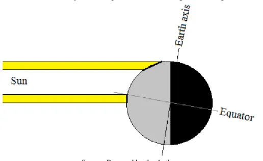
Figure 7 – Radiation intensity in the Equator and Polar regions during Southern summer
Source: Prepared by the Author.
Geographical position on earth as distance from the equator results in a different intensity of solar radiation (Figure 7). This is due to the changes of the Sun’s position and the length of daylight caused by the tilt of the Earth’s axis relative to the orbital plane.
Figure 8 displays the amount of solar radiation throughout the year at two different locations on earth, Fortaleza Brazil and Kassel Germany.
Figure 8 – Annual distribution of solar radiation at Fortaleza Brazil and Kassel Germany
Source: Universität Kassel (2003).
and double of that with 2000 kWh/m2 in Fortaleza Brazil. A peak is found in the Sahara with up to 2500 kWh/m2 per year (Table 1).
Table 1 – Solar radiation energy per m2 on horizontal surfaces at different locations Location kWh/2 per year
Kassel 1000
Thailand 1700 – 1800
Brazil 2000
Sahara 2200 – 2500
Source: Universität Kassel (2003).
The radiation energy on reaching the earth’s surface is converted mainly into heat.
A smaller fraction is consumed by plants’ photosynthesis for cracking up CO2 of the air and converting it into oxygen and biomass in form of carbohydrates, e.g. C6H12O6. Fossil forms of energy like petrol, natural gas and coal are prehistoric biomasses that where compacted and sealed deep beneath the earth surface for millions of years.
Heat for its part causes evaporation of water and drives the global and regional wind systems which transport the moisture with the floating air masses (the wind) to distant places where it is occasionally dumped as precipitation (rain), thus, providing water that is required for all living beings all over the earth. In a similar manner, the surface waters of the ocean are heated causing sea-currents around the world coming from equatorial regions and heating northerly and southerly regions like northern Europe with the Gulfstream.
Biomass was always the sole physical energy source for animals and humans. Cooking with firewood is a prehistoric technique used by humans until today. The more advanced use of other forms of energy started most probably with the sailboats some estimated 5000 years ago, followed later on by windmills in Babylonia and China and finally with wind- and water mills in Europe using wind and rivers as energy source. In parallel, biomass has been used widely to provide energy for domesticated working animals, especially horses in order to substitute human muscle work for thousands of years (MANN, 1986).
reserves, mainly coal, petrol and gas and the development of combustion engines that convert liquid and gaseous fuels into mechanical work (LILJEDAHL, 1989).
Today, humanity has run into serious problems with this development. Pollution and the increase of CO2 in the atmosphere are causing climate change and are a serious threat to human existence. The sustainable development, defined by the United Nations (UNO.
1987) is not achievable by continuing today’s practice to burn gigantic amounts of fossil
fuels. Developed societies are conscious of that peril and science and industry are developing alternative ways to power machines with renewable energies at a global scale (HINDRICH, KLEINBACH, 2004).
The wide use of renewable energy started with electrification more than a century ago by using the gravitational potential energy of water in rivers to generate electricity. Dams were built to impound water as a type of potential energy storage which can be converted in electricity in a controlled manner (MANN, 1986).
Nowadays, all possible types of transformation of renewable energy into usable energy forms are investigated. However, so far only wind turbines conquered a bigger market share in electricity generation (ACKERMANN, 2005).
A very promising technology is the direct conversion of solar radiation into electrical energy by photovoltaic systems. The perspective is that this technology will be the most economic method of electricity generation in the very near future (Agora 2015).
2.5 Photovoltaic
In a photovoltaic device (abbreviated PV) a direct transformation of solar radiation energy into electrical energy occurs. The radiation energy interacts directly with the
electrons of the atoms constituting the solar cell’s crystals. Alexandre Edmond Becquerel
discovered this photovoltaic effect in 1839.
A solar cell of the most widely used type comprises two silicon layers, one doped with boron (B), a trivalent element and one doped with phosphorous (P), a pentavalent atom, as shown in Figure 9 (BERGELT, 2012).
Figure 9 – Doping of silicon: (a) with the pentavalent atom (Phosphor) and (b) with the trivalent atom (Boron)
Source: Bergelt (2012).
An electric potential is created because there is an electron excess on the phosphorous layer (n – positive type of material) with many free electrons and a lack of electrons on the boron layer (p – negative type of material) with many holes (Figure 10). At the interface between these two layers the charge potential differences lead to the phenomena that electrons from the n-region diffuse into the p- region and holes from the p-region diffuse into the n-region.
Figure 10 – Charge carrier distribution at p-n junctions and currents through the junction
The electrostatic fields extending over the boundary surface represent a potential difference, the diffusion voltage. When light falls on the solar cell, the photons excite the electrons. This is named the photoelectric absorption. When the photons energy is completely captivated by a bound electron, it becomes a free-electron.
Figure 11 – Operating principle of solar cells (schematic)
Source: Universität Kassel (2003).
A photon with sufficient energy penetrates the emitter, the n-type layer of the solar cell and is absorbed in the base, the p-type layer (Figure 11). An electron-hole pair develops due to the absorption. The free electron diffuses in the p-base until it arrives at the boundary of the space-charge zone. Subsequently, the electric field in the space-charge zone accelerates the electron and transports it to the emitter side (GREENPRO, 2003).
As the concentration of electrons at the n-emitter side growths, the number of holes at the p-base side growths correspondingly. Consequently, an electrical voltage builds up. If n-emitter and p-base are now connected via an electric load, electrons flow. This current
flow continues as long as the sun’s radiation continues to excite the electrons of the solar cell.
Hence, solar radiation energy is directly converted into electrical energy (UNIVERSITÄT KASSEL, 2003).
Icell = Iph – ID (1) where:
Icell = Solar Cell current [A]; Iph = Photocurrent [A]; and ID = Diode current [A].
Figure 12 – Equivalent circuit diagram of a solar cell connected to a load
Source: Universität Kassel (2003)
Today’s commercial grade solar panels have an efficiency of up to 18% and a
lifetime expectancy of 20 to 30 years.
2.6 Wind energy
Wind is a mass of air in movement. It represents a form of kinetic energy (Equation 2).
𝐸 = 𝑚𝑣22 (2)
where:
The wind turbine is a device that extracts a major fraction of this kinetic energy aerodynamically and converts it via a mechanically driven generator into electric energy (GASCH, 2007).
Daniel Bernoulli (1700-1782) together with Leonhard Euler (1707-1783) discovered the laws of aerodynamics according to which the sum of the different forms of energy of a fluid in motion has to be constant (Equation 3).
𝑣2+ 𝑔ℎ + 𝑝 ρ⁄ = 𝑐𝑜𝑛𝑠𝑡𝑎𝑛𝑡 (3)
where:
v = velocity [m/s];
g = acceleration of gravity [9.8 m/s2]; h = height [m];
p = pressure [N/m2]; and ρ = density of the fluid [kg/m3].
Figure 13 –Bernoulli’s scheme of dynamic flow in a tube
Source: Prepared by the Author
Consequently, in a flow of air forced to accelerate, the pressure drops to maintain the energy balance (Figure 13).
This is the effect that wings of a bird, a plane and the rotor blade of a wind turbine use to generate physical forces. At a wind turbine, these forces are used to drive the rotor disc. Via a mechanical link, i.e. gearbox, the rotational speed is increased to drive an electric generator. Large size wind turbines may also use direct-driven generators (CARVALHO, 2003).
already upstream of the rotor plane and continues to do so after passing it. The pressure consequently increases upstream of the rotor plane with a sharp drop when passing it (which is actually the force that moves the blade) and equalizes to the surrounding air pressure after passing the plane of the rotor (BURTON, 2003).
Downstream of the rotor plane, the cross sectional area of the air mass flow increases further, and the air mass continues to decelerate (Figure 14) for a certain distance, up to a point where turbulence mixes the air passing through the turbine with the surrounding air mass.
Figure 14 – Air flow tube near the blades of a wind turbine
Source: Prepared by the Author
In Physics, it is expressed as the mass is constant in (Equation 4):
𝜌𝐴∞𝑣∞ = 𝜌𝐴𝑑𝑣𝑑 = 𝜌𝐴𝑤𝑣𝑤 (4)
where:
ρ = density of air [kg/m3]; A = area of mass flow [m2]; and v = velocity [m/s].
Figure 15 – Wind turbine at an elevated position
Source: Prepared by the Author
2.7 Local renewable electric energy systems
2.7.1 Electric Fundamentals
By powering a device, a motor or engine (prime mover) performs in terms of physics mechanical work. To enable the motor to perform this mechanical work, energy is to be made available. This can be in the form of chemical energy or as investigated in this document electrical energy.
Electrical energy is generally made available to electrical consumers by connecting them via a transmission system to a power generation plant, i.e. the power generated is consumed at the same moment. This is the preferred concept since storage of electrical energy requires cost intensive technical devices.
All electrical phenomena are caused by electrical charges. An electrical charge is a basic physical property and is expressed in Coulomb [C] which represents a current of 1 Ampere that passes through an electrical conductor in 1 second.
[Q] = Coulomb = C = As
All electrical charges are composed of elementary charges [e]:
e ≈ 1602 * 10-19 C
An electrical current is a flow of electrical charges [Q] that pass a cross section of the conductor (Equation 5) during a defined time interval [t]. The strength of the electric current is named amperage [I]:
𝐼 = ∆𝑄∆𝑡 (5)
where:
I = Current [A]; Q = Coulomb [C]; and t = time [s].
The flow of charges occurs usually through an electrical conductor. An electrically conductive material is characterized by free moving electrons. When an electrical tension is applied to a conductor these negative charges move in form of a current from the negative side to the positive side of the conductor. However, technically the flow direction of the current is considered from positive to negative as if positive charges would be freely moving from the positive side to the negative side.
This ohmic resistance of a conductor is calculated as (Equation 6):
R(conductor) = ρ(conductor)
∗
𝐴𝑙=
𝐾(𝑐𝑜𝑛𝑑𝑢𝑐𝑡𝑜𝑟)∗ 𝐴𝑙 (6)where:
R = resistance [Ω];
ρ = specific resistance [Ωmm2/m]; K = specific conductivity [Sm/mm2]; A = cross-section [mm2]; and
l = length of the conductor [m].
Metals have free moving electrons and silver, copper, gold and aluminum have the highest specific conductivity, but for economic reasons only copper and aluminum are commonly used for electrical conductors. Hence, when a current flows a part of the transitory energy is converted into heat.
The heat represents the loss of power and is calculated as given below by Equation 7:
Ploss = I2 * R (7)
where:
Ploss = Power loss [W]; I = Current [A]; and
R = Resistance [Ω].
For determining the current the following formula applies (Equation 8):
I = P/U (8)
where:
I = Current [A];
P = Total power [W]; and
According to the above given formulas, the power loss depends on the conductivity but even more on the voltage because a higher voltage reduces the amperage of the current (with power constant) which enters with the square in the power loss calculation.
The use of renewable energy in rural areas is increasing, but since wind and sun are an inconstant source, the combination of a low-cost renewable technology with common technology via a grid connection provides a solution. Those hybrid power systems incorporate different components as generation, storage, power conditioning and system control (ACKERMANN, 2005).
The classic hybrid system includes both a direct-current (DC) bus with a battery bank and an alternating-current (AC) bus and a backup engine generator (if grid connection is not available). Small isolated systems use batteries to store surplus energy and the battery bank acts as power dampener, smoothing out fluctuations in the power flow.
Figure 16 illustrates a DC-bus power system providing AC power via a power converter. The backup generator can also be operated with biogas (if biogas is available and the engine is adapted to burn it). The bidirectional inverter offers the possibility to connect the system to the grid (if available) for backup power supply or alternatively to store surplus energy (ACKERMANN, 2005). In this case, the system can be operated without a battery bank.
Figure 16 – System with connection to public grid
2.7.2 Transmission and conversion/inversion
Renewable energy systems with a small wind or PV generator but without battery storage are connected directly to the consumer. This applies for instance for minor loads such as ventilators or small water pumps (Figure 17 a).
Systems with a converter are applied if the voltage of the generation system has to
align with the voltage of the consumer. A DC/DC boost converter transforms the generator’s
DC voltage to the DC voltage of the consumer (Figure 17 b).
Figure 17 – Configuration of (a) direct coupled system and (b) system with DC-DC boost converter
Source:Universität Kassel, 2003
An AC system uses converters, which transform DC power into AC power. This kind of system is commonly used for electrical loads and electrical motors consuming more than 2 kW (Figure 18).
Figure 18 – Configuration of a system with DC-AC converter
Source:Universität Kassel, 2003
Figure 19 – Configuration of a system connected to the grid
Source:Universität Kassel, 2003
Systems with battery storage (Figure 20) generally have to use a charge regulator to protect the batteries from overcharge and deep discharge (DDP). This is to ensure the longest possible battery life.
Figure 20 – Configuration of a DC-coupled system with battery backup
Source:Universität Kassel, 2003
For systems with battery storage and higher power needs (in conventional households with AC consumers or in the case of industrial electrical devices), an AC-DC-inverter has to be included (Figure 21).
Figure 21 – Configuration of a system with an AC consumer
This type of system normally combines a back-up generator (Figure 22) to safeguard power supply when the batteries are discharged and sun and wind are temporarily not available as energy sources.
Figure 22 – Configuration of a hybrid system with backup generator
Source:Universität Kassel, 2003
2.7.3 Storage systems
A central issue with electrical energy is that it is hard to store it at a high power density (like chemical energy in the form of petrol).
The most common mobile energy sources used by electric vehicles are usually chemical batteries, whereas capacitors are usually intermediate energy storage devices building up brake energy to release it for propulsion when indicated.
A capacitor is an electrical component that stores electrical energy in an electric field. Two electrical conductors of a circuit in sufficient close proximity are separated with a dielectric insulation material. When the two conductors experience a potential difference, an electric field develops causing a positive charge on one side and a negative charge on the other side. If a varying voltage is applied a current is caused to flow through the connected circuit.
Batteries rely on chemical processes to store electric energy during the charging cycle or supply electric energy during the discharge cycle. Basically, an electrochemical battery consists of three primary elements: two electrons (positive and negative), immersed in the electrolyte (Figure 23).
Figure 23 – A typical electrochemical battery
Source: Mehrdad (2010).
Batteries are specified by their coulometric capacity in Ampere-Hours, i.e., as ampere-hours provided when discharging the battery from fully charged until it is down to its cut-off voltage (Figure 24).
Figure 24 – Cut-off voltage of a typical battery
An important characteristic in terms of battery capacity is the number of ampere-hours vs different discharge current rates. With a higher discharge rate, the capacity generally decreases significantly (Figure 25).
Figure 25 – Discharge characteristic of a lead-acid battery
Source: Mehrdad (2010).
A common example of an electrochemical reaction in batteries used in vehicles is the lead-acid battery (Figure 26). It uses an aqueous solution of sulfuric acid (2H+ + SO
4-2) as electrolyte. The electrodes are of porous lead (Pb) in case of the anode (-, negative) and porous lead oxide (PbO2) in case of the cathode (+, positive).
Figure 26 – Electrochemical process of a lead acid battery cell: (a) discharging and (b) charging
Source: Mehrdad (2010).
The chemical reaction on the anode during the discharge phase is: Pb + SO-2
4
electrode. By the flow of electrons through an external circuit to the positive cathode electric energy is generated to power a load (for example in form of an electric motor).
At the positive electrode, PbO2 is converted to PbSO4 and water is produced. Charging reverses the chemical reaction on the anode and cathode.
Cycle life of batteries
Battery cycle life is the capability of the battery to endure a specific number of charge/discharge cycles. The depth of discharge (DOD) is a critical figure in battery life. The typical lead-acid battery in an automobile has a limited cycling capability of less than 100 nominal cycles of deep discharges.
However, as the lifetime of a battery depends not only on the cycles but as well on the depth of discharge (expressed as a percentual of the rated deep discharge capacity), a battery with a nominal 100 cycles of deep discharges is able to endure 500 cycles of 20% discharge depths (Figure 27 and 28). This can roughly be expressed by:
Nominal cycles of battery life = actual cycles * (depth of discharge [%] / 100)
Battery capacity is normally expressed in Ah (Ampere-hours), but energetic content is more precisely defined in Wh (Watt-hours). These values are related with the battery voltage through the equation:
I (A) * U (V) * t (h) = E (Wh)
Figure 27 – Cycle life as a function of depth of discharge for different types of batteries
Figure 28 – Cycle life versus depth of discharge DOD of Ni/Cd cells
Source: NASA (1987).
Apart from the number of load cycles, capacity is also affected by temperature with about 1% capacity loss per degree below about 20°C. On the other hand extremely high temperatures decrease capacity too, accelerate aging, and self-discharge (Figure 29).
Figure 29 – Cycle life as a function of depth of discharge DOD and temperature of Ni/Cd cells
Source: NASA (1987).
efficiency and lifetime (see Table 2). Furthermore, aspects like self-discharge, maintenance requirements, reliability, mechanical integrity and safe operation have to be considered.
Table 2 – Costs, energy and efficiency comparison of different battery types Type Cycle live for
80% DOD
Investment cost
(€/kWh) cost (€/kWhSpecific kWh )
Self-discharge [%/month]
Temp-range [°C]
Pb 1500 ... 3500 85 ... 350 0.17 ... 0.30 >80 -15° to +50° NiCd 1500 ... 3500 650 ... 1500 0.30 ... 1.00 71 -40° to +45°
NiFe 3000 1000 0.33 40 -0° to +40°
Source: Universität Kassel (2003).
The type of battery widely used since a century is the lead-acid battery. But actually the battery favored for mobile use is the Li-ion battery because of its superior performance with respect to energy density and its load and discharge characteristic. Compared to lead-acid, the Li-ion battery has a higher energy density (Figure 30), a better charge and discharge characteristic and is expected to become the most economical alternative for mobile use in the near future.
Figure 30 – Energy density comparison of batteries
2.7.4 Motors
Electric motors exhibit a different torque, speed and power characteristic as compared to combustion engines. The design of an electric vehicle has to consider these specific properties which result in a different configuration and layout of the drive train. Especially the torque and speed characteristic of an inverter controlled squirrel cage induction motor exposes a significant difference to a combustion engine as shown in the graphic below (Figure 31).
Figure 31 – Typical torque characteristic of combustion engine vs. electric motor
Source: Prepared by the Author.
Whereas the torque curve of the combustion engine reaches a peak next to the maximum speed nmax, the electric motor delivers its nominal torque Mn from standstill no to nominal speed nn.
To Mehrdad (2010), the “variable-speed electric motor drives usually exhibit the characteristic that in the low-speed region (up to nominal speed), the motor has a constant torque. In the high-speed region (over nominal speed), the motor has constant power”.
Figure 32 – Forward and reverse torque characteristic of an electric motor
Source: Strategien zur Elektrifizierung des Antriebsstranges (p.92).
Another characteristic of the electric motor that has a significant influence on the
tractor’s pull characteristic is its torque reserve. For a limited time, it is able to generate several times the nominal torque (see Figure 31 –“Electric motor torque reserve”).
A common configuration to power an electric vehicle is a squirrel cage induction motor controlled by a frequency inverter which draws the required energy from the onboard battery (Figure 33).
Figure 33 – Electrical vehicle onboard electric architecture
Source: Prepared by the Author.
2.7.5 Inverters and converters
Inverters are electrical current power-conditioning elements. They invert the direct current of an electric energy source in an alternating frequency (AC). Some renewable energy system components like photovoltaic systems (PV) and batteries operate with direct current (DC) but the majority of electrical consumer equipment is running on alternating current (AC). A device (inverter) is required to link the two systems.
Apart from that, inverters align voltage and frequency of decentrally generated electrical energy with the public grid, and therefore allow its injection into it. Finally, yet importantly, inverters make it possible to control the speed and torque of AC electric induction motors. Those motors, when connected to the public grid without an inverter, synchronize with the grid frequency and can rotate only at the fixed, not variable speed of the grid voltage frequency.
The symbol used to describe an inverter is shown in Figure 34. The input is a direct current while the output is an alternating current.
Figure 34 – Symbols to describe: (a) inverter and (b) converter
Source: Universität Kassel, 2003
Inverter principles