DESIGN TO LEARN: CUSTOMIZING SERVICES WHEN THE FUTURE MATTERS
Dan Ariely
1, Gabriel Bitran
2and Paulo Rocha e Oliveira
3* Received April 25, 2012 / Accepted May 10, 2012ABSTRACT.Internet-based customization tools can be used to design service encounters that maximize customers’ utility in the present or explore their tastes to provide more value in the future, where these two goals conflict with each other. Maximizing expected customer satisfaction in the present leads to slow rates of learning that may limit the ability to provide quality in the future. An emphasis on learning can lead to unsatisfied customers that will not only forego purchasing in the current period, but, more seriously, never return if they lose trust in the service provider’s ability to meet their needs. This paper describes service design policies that balance the objectives of learning and selling by characterizing customer lifetime value as a function of knowledge. The analysis of the customization problem as a dynamic program yields three results. The first result is the characterization of customization policies that quantify the value of knowledge so as to adequately balance the expected revenue of present and future interactions. The second result is an analysis of the impact of operational decisions on loyalty, learning, and profitability over time. Finally, the quantification of the value of knowing the customer provides a connection between customer acquisition and retention policies, thus enhancing the current understanding of the mechanisms connecting service customization, value creation, and customer lifetime value.
Keywords: Service customization, customer learning, customer lifetime value, dynamic programming.
1 INTRODUCTION
Electronic interfaces for service delivery present unprecedented opportunities for customization. Companies can identify returning customers at almost no cost and present each of them with a unique interface or service offering over a web page, voice interface, or mobile device. Cus-tomization is important in these interactions because the variety of products, services and in-formation that companies can offer can be enormous and customers are often not able to find and identify the alternative that best suits their preferences. More generally, the amount of in-formation available over the Internet is overwhelming and the costs to search and evaluate all potentially relevant pieces of information can be prohibitive.
*Corresponding author
1Duke University – Fuqua School of Business, 2024 W. Main Street, Durham, NC 27705. E-mail: [email protected] 2MIT – Sloan School of Management, 77 Massachusetts Avenue, Cambridge, MA 02042, USA.
E-mail: [email protected]
This situation can lead to interactions of low net utility to customers. Hence the need for soft-ware applications generally called intelligent agents (or smart agents) that present customers with customized recommendations from large sets of alternatives. These agents have the potential to create great benefits for both consumers and companies. It is certainly desirable for customers to reduce search costs and by going directly to a company that already knows them and gives them high utility. At the same time, companies that learn about their customers can use this knowl-edge to provide increasingly better service as the relationship progresses, making it difficult for competitors to “steal” their customers.
In order to fully reap the benefits of customization, companies must overcome two obstacles. First, the strategies that maximize selling (or their customers’ utility in the current period) do not coincide with strategies that maximize learning. Second, the cost of making bad recommenda-tions (and learning form them) might be prohibitive because customers rarely forgive and return to service providers that make bad recommendations. Overcoming these obstacles depends on the agents’ ability to adequately balance the goals of learning at the expense of selling and selling at the expense of learning.
In addition to being an important tool in the reduction of search costs, smart agents are also cost-efficient. Consequently, as more and more services are delivered through automated interfaces, smart agents have been playing increasingly important roles in everyday decision-making and are gaining considerable more autonomy to act on the consumers’ behalf (Maes [1995] documents the early days of this tendency).
The essential task of learning about customers in order to provide better recommendations has been made more difficult in many ways as interfaces change from human to human-computer. Human intermediaries can, in many cases, observe their clients and make a number of inferences on the basis of their interactions. The lack of cues typical of the personal encounter di-minishes the opportunities for correcting incomplete advice or wrong guesses. Software agents only register click patterns, browsing behavior, and purchase histories. These agents can only learn about customers by asking them questions and by observing their behavior. The issues related to the benefits and limitations of asking questions have been adequately addressed else-where: clients may not be willing nor have the patience to answer questions (e.g., Toubiaet al., 2003), and their replies are not always truthful for various (and sometimes intentional) reasons (White, 1976). Regardless of how they answer surveys, customers spend their time and money in the activities from which they derive the most utility. In the offline world, Rossiet al.(1996) found that the effectiveness of a direct marketing campaign was increased by 56% due to the cus-tomization of coupons based on observations of one single purchase occasion. Intelligent agents can learn about customers by observing the purchases they make. Furthermore, firms interacting with customers through automated interfaces can also lean by observing the products that cus-tomer reject. Therefore, companies must strive to learn about their cuscus-tomers by observing how they react to the recommended products and services to which they’re exposed.
their customers to like and learn about their customers’ preferences at slow rates or they can take more risks by suggesting products their customers might not accept and learn at higher rates. The agent’s dilemma captures the essence of the selling versus learning trade-off faced by companies that customize services on the Internet. Observing an action that was already expected to happen only reconfirms something one already knew or suspected to be true. But should an agent recommend a product with no prior knowledge of how their customers would react? By taking this course of action, agents may learn a lot about their customers’ responses to recommendations of such products, regardless of whether or not the item is purchased. However, they run the risk of causing an unsuccessful service encounter that may lead to defection. Customers who receive very bad recommendations can lose trust in the smart agent’s ability to help them make better decisions and never return. Research in psychology and marketing has repeatedly shown the importance of trust as the basis for building effective relationships with customers in e-commerce as well as in regular commerce (e.g., Kollock, 1999; Lewickiet al., 1998; Arielyet al., 2004). Doney & Cannon (1997) established an important link between trust and profitability by noting the importance of trust to build loyalty. Low trust leads to low rates of purchase, low customer retention and, consequently, meager profits. Studies on human and non-human agents have extended the findings of previous research by showing that trustworthy agents are more effective,i.e., they are better at engaging in informative conversation and helping clients make better decisions. Urbanet al.(2000) have also shown that advice is mostly valued by less knowledgeable and less confident buyers, and those are exactly the same customers less likely to trust external agents to act as surrogates on their behalf. The human element involved in company-customer relationships makes it imperative that firms strive to build and maintain trust if they are to maintain profitable customers in the long run. The question is how these principles can be operationalized in the strategies adopted by agents.
advice are lower, yet the electronic agent must rely on much more precarious information and cues regarding consumers’ tastes and preferences.
The customization policy used by the agent affects the customer lifetime value (CLV) in two ways. CLV is typically defined as the net present value of the stream of cash flows the firm expects to receive over time from a given customer (e.g., Berger & Nasr, 1998; Jain & Singh, 2002). The customization policy determines expected quality, which in turn influences (1) the customer defection decision and (2) the expected revenue per interaction. The model analyzed in this paper does not make any assumptions about the retention rate and profitability as the rela-tionship progresses. These parameters are determined by the business setting and the manager’s decisions. This flexibility is an important contribution of this paper, as it presents a tool that can accomodate situations where profits accelerate over time as well as those when profits do not accelerate over time.
The next section of this paper formalizes the customer behavior model, describes the dynamics of customer/company interactions, and formulates the agent’s customization problem as a dynamic program. Section 3 establishes the optimality conditions and solution procedures for the model introduced in Section 2. Section 4 discusses the significance of the results, paying close attention to their meaning in the context of CLV research. Finally, Section 5 offers some directions for further research.
2 MODEL DESCRIPTION
This section is divided into three parts. The first one presents a mathematical choice model that captures the essential behavioral features of the choice process customers go through when interacting with software agents. This is followed by a description of a dynamic system used to model the interactions between customers and companies over time. The third part shows how the company’s decision of how to customize products and services can be framed in terms of a Markov Decision Process using the customer behavior model of Section 2.1 and the dynamical system of Section 2.2.
2.1 Customer Behavior
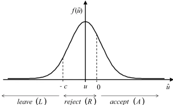
This section describes a customer behavior model that captures the ways in which customers react to recommendations of products and services made by software agents that is consis-tent with the behavior qualitatively described in the psychology and marketing literature (e.g., Zauberman, 2000; Ariely et al., 2004). Customer observe the true quality of the recommen-dation, plus or minus an error term. The probability that the customer will accept the recom-mendation, reject the recomrecom-mendation, or leave the company is defined through a random utility model (e.g., McFadden, 1981; Meyer & Kahn, 1990). According to random utility theory, when a customer is offered product X the utility that is actually observed has two components: a de-terministic componentu(X), which corresponds to the true underlying utility and an error term
measurement errors that make the customer unable to determine the exact utility of a product upon initial examination. Formally, this can be expressed as
ˆ
u(X)=u(X)+ε
whereuˆ(X)is the observed utility.
Once customers evaluate the utility ofX, the service they are being offered, they can take one of three actions:
• Accept productXifuˆ(X) >0
• Reject product but come back next time if−c<uˆ(X) <0
• Leave the company and never come back ifuˆ(X) <−c
Customers who observe a very low utility (−c, which can be interpreted as a switching cost) immediately lose trust in the agent as a reliable advisor and never return. In the case of services provided over smartphone apps, this can be interpreted as unistalling the app. The recommenda-tion is accepted if the observed utility exceeds a given threshold, which can be assumed to be 0 without loss of generality. Customers who accept the suggested product or service are satistfied and return the next time they require service. If a recommendation is barely below the accep-tance level, customers will purchase elsewhere (or forego purchasing in the current period) but return in the future. The cost of not making a sale by experimenting with different customization policies is captured by the probability that the observed utility will fall in the interval[−c,0]. The probabilities of accepting, leaving, or rejecting a productX (denoted pA(X), pL(X), and
pR(X), respectively) can be computed by defining the distribution ofε. Ifε is normally dis-tributed with mean 0 and varianceσ2, the parameterσ can be altered to represent different types of products or business settings, where the customer observes products with more or less error. This model corresponds to the ordered Probit model, and its properties are thoroughly discussed in Greene (2000). The general formulation of the choice probabilities is shown in the first column of (1), and the specific form they take whenε∼N(0, σ )is shown in the second column (where 8represents the cumulative normal function). Figure 1 depicts the probabilities taking each of the three possible actions when the customer is offered a recommendation with a deterministic utility component u. In this particular case,u is below the acceptance threshold, but since the observed utility isu+εthe probability that the product will be accepted is positive.
Action Probability of Action Probability ifε∼N(0, σ )
Accept pA(X)=Pr(u(X)≥0) =8u(σX)
Leave pL(X)=Pr(u(X) <−c) =8−u(Xσ)+c
Reject pR(X)=
1−pA(X)−pL(X)
=1−8u(σX)−8−u(Xσ)+c
−
0
ˆ
)
ˆ
(
( )
( )
( )
Figure 1– Probabilities of Accepting, Rejecting and Leaving when offered a product with deterministic utilityu.
2.2 Dynamics of Customer-Company Interactions
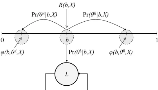
Figure 2 describes the dynamics of customer/company interactions. Since the interactions take place through an automated interface controled by a smart agent, the words “company” and “agent” are used interchangeably. This system is the basis of the formulation of the agent’s dilemma as a Markov decision problem.
Figure 2– The dynamics of customer-company interactions.
thei’th component of the prior belief vector isbi0=Pr(S∗ =Si)∈ [0,1]. Since all customers must belong to some segment,
|S| P
i=1
b0i = 1. The learning problem faced by the agent is the assignment of an individual customer to one of the|S|segments.
Each segmentSiis defined by a utility functionui(X)that maps products and servicesXinto real numbers. One way to define these utility functions is by associating each segmentSiwith a vector βi. The components ofβi are the weights a customer of segmentigives to each attribute of the products in X. The corresponding utility function could be defined as ui Xj =
β′i∙Xj
, whereui Xjdenotes the utility that productXj has to a customer of segmentSi.
When the customer requests service, the company chooses a product from the setX = {X1,
X2, . . . ,X|X| . Xis a set of substitute products or services, and can be thought of as the
dif-ferent ways in which a service can be customized. Each Xi ∈Xis a vector whose components correspond to different levels of the attributes of the product or service. The recommendation made during thet’th interaction is denotedXt. The decision problem of which service configu-ration should be chosen is directly addressed as an optimization problem in Section 2.3. The customer will either accept the recommendation, reject the recommendation, or leave, as explained in the beginning of this section. The probabilities with which each of these actions take place are given by (1). The company will observe the customer’s action as described in Figure 2. The observation made during thet’th interaction is denotedθt, and the set of possible observations is2 =
θA, θR, θL , corresponding to accepting the recommendation, rejecting the recommendation, and leaving the system. For example,θ5 =θAmeans that the customer accepted the product offered during the fifth interaction.
After each observation, beliefs are updated in light of the previous belief and the action/observ-ation pair of the last interaction. Bertsekas (1995a) proved that the last belief,bt−1is a sufficient statistic for b0,X1, θ1,X2, θ2, ...,Xt−1, θt−1
. Thus, ifbti denotes thei’th component of the belief vector aftert interactions, then
bit =PrS∗=S1|bt−1,Xt, θt
.
The new belief can be computed using
PrS∗=Si|bt−1,Xt, θt
= 1
Pr θt|bt−1,Xt∙ h
bti−1∙Pr θt|Si,Xt i
where
Prθt|bt−1,Xt= |S| X
i=1 h
bit−1∙Pr θt|Si,Xt i
(2)
is a normalizing factor. The update functionϕcan then be defined by
ϕ (b, θ ,X)= 1
Pr(θ|b,X)∙
b1∙Pr(θ|S1,X)
b2∙Pr(θ|S2,X) ...
b|S|∙Pr θ|S|S|,X
2.3 Optimization Problem
The company earns a payoff of 1 if the customer accepts the recommendation and 0 otherwise. Since increasing the utility always increases the probability of purchase, the incentives of the customer and the company are perfectly aligned. It is always in the company’s best interest to please the customer, since the more utility the company provides to the customer, the higher the payoff. The expected payoff of suggesting product Xj to a customer from segment Si is given by
R Si,Xj=1∙piA Xj+0∙piR Xj+0∙piL Xj=piA Xj (4) where piA Xjis the probability of purchase as defined in (1).
If the company knows the customer’s true segment, the problem of making recommendations reduces to always suggesting the product with the highest expected utility for that segment. This is a Markov chain model, which can be easily extended to other models such as those of Pfeifer & Carraway (2000) through state augmentation.
The problem of making recommendations is not as simple if the company does not know the customer’s segment. The real decision is to find the best recommendation for each possible belief so as to maximize the expected revenue (or customer’s utility). This policy, denotedμ∗ must solve the equation
μ∗=arg max X∈X
( E
∞ X
t=0 γtrt
!)
(5)
whereγ ∈ (0,1)is a discount factor andrt is the reward at timet. The set of possible beliefs is[0,1]|S|, which is uncountably infinite. This stands in sharp contrast with customer migration
models, where the possible states of the system are defined by a finite (or countably infinite) set. In the belief-state problem, the payoff function maps belief states and actions to revenues. There-fore, the payoff functionR˜is defined by
˜
R(b,X)= |S| X
i=1
bi ∙R Si,Xj. (6)
The three possible transitions from any given belief state are given by
Prbt = ˆb|bt−1,Xt=
|S| P
i=1
bti−1∙piA Xt
if bˆ=ϕ bt−1, θA,Xt |S|
P
i=1
bti−1∙piR Xt
if bˆ=ϕ bt−1, θR,Xt |S|
P
i=1
bti−1∙piL Xt
if bˆ=ϕ bt−1, θL,Xt =L
0 otherwise
(7)
Pr Pr
Pr
Figure 3– Transition probabilities and payoffs in the partially observable stochastic shortest path problem.
The optimal value functionV∗(b)=maxE
∞
P
t=0 γtrt
satisfies the Bellman equation
V∗(b)=max X∈X
( ˜
R(b,X)+γ X b′∈B
P b′|b,X V∗ b′
)
. (8)
We know from (8) thatb´can only take three possible values, namelyϕ b, θA,X,ϕ b, θR,X, andϕ b, θL,Xt
.Furthermore, since customers have no value after they leaveV∗(L)=0. Therefore, (9) can be written as
V∗(b)=max X∈X
˜
R(b,X)+γ X
θ∈{θA,θR}
P(θ|b,X)V∗(ϕ (b, θ ,X))
, (9)
The dynamic programming mapping corresponding to the above value function is
(T V) (b)=max X∈X
˜
R(b,X)+γ X
θ∈{θA,θR}
P(θ|b,X)V∗(ϕ (b, θ ,X))
(10)
This mapping is a monotone contraction under the supremum metric. Therefore, repeated ap-plication of the operatorT to a value functionV converges to the optimal value function (e.g., Bertsekas, 1995b). This result is the basis for the value iteration algorithm, which consists of repeatedly applying the operatorT to the value functionV1. LettingVn=TnV,i.e.,n applica-tions ofT toV1, then the algorithm is stopped when|V∗(b)−Vn(b)|is within a tolerable error margin, which can be expressed as a function of|V∗(b)−Vn−1(b)|(this is an application of a standard result found in Littman [1994] or Bertsekas [1995b], for example).
mean that there exists some n for which Vn cannot be represented finitely or that the value function updates cannot be computed in a finite amount of time. The next sections describes how these difficulties can be overcome in order to solve the agent’s dilemma.
3 MODEL ANALYSIS AND SOLUTION
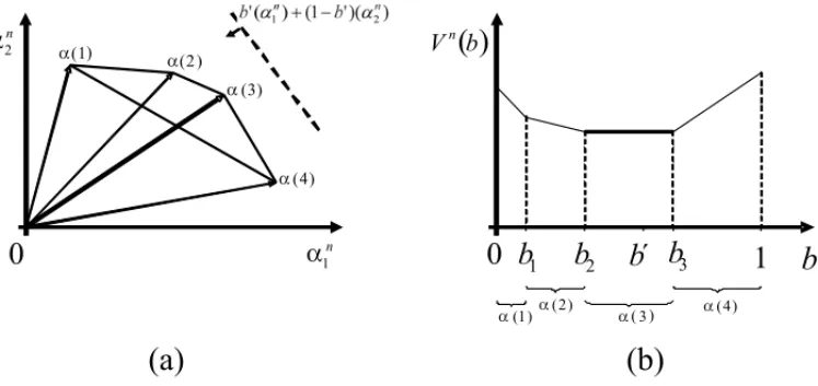
The value function aftern iterations of the dynamic programming mapping is piecewise linear convex function and can be written as
Vn(b)=max a∈An(b∙α)
where Anis a finite set of|S|-dimensional vectors. This implies thatV∗(b)can be approximated arbitrarily well by a piecewise linear convex function.
Proposition 1. The value function Vn(b), obtained after n applications of the operator T to the value function V1(b), is piecewise linear and convex. In particular, there exists a set An of |S|-dimensional vectors such that
Vn(b)=max a∈An(b∙α)
Proof. The proof is by induction, and therefore consists of the verification of the base case and of the induction step.
(1) Base case:V1(b)=max
α∈A1(b∙α) .
(2) Induction step: If
∃An−1such thatVn−1(b)= max
α∈An−1(b∙α)
then
∃Ansuch thatVn(b)=max
α∈An(b∙α) .
The statement above can be proved by verifying that the elementsα∈ Anare of the form
α= pA(X)+γ ŴA(αi)+γ ŴR αj (11)
whereαi ∈ An−1,αj ∈ An−1andŴAandŴRmatrices with elements
Ŵi jA(X)=
piA(X) ifi = j
0 otherwise
and
Ŵi jR(X)=
pR(X) ifi = j
It then follows that
Vn(b)=max
α∈An(b∙α)
which can be verified to be true by defining
An:= [
X∈X
[
αi∈An−1
[
αj∈An−1
pA(X)+γ ŴA(X)∙αi+γ ŴR(X)∙αj
.
The details of the proof are in Appendix A.1.
Figure 4a shows an example of the convex hull of a hypothetical setAnconsisting of four vectors and Figure 4b depicts the corresponding value functionVn(b). Each vector corresponds to a different customization policy. On a more intuitive level, each component of the vector is the expected payoff the agent would receive given a sequence of recommendations and a customer segment. The optimal policy will be a function of the belief (represented by the slope of the dotted line in Figure 4a) and the set of feasible policies. Each piecewise-linear segment of the value function 4b corresponds to a different policy.
Figure 4– A set ofAnvectors and their corresponding value function.
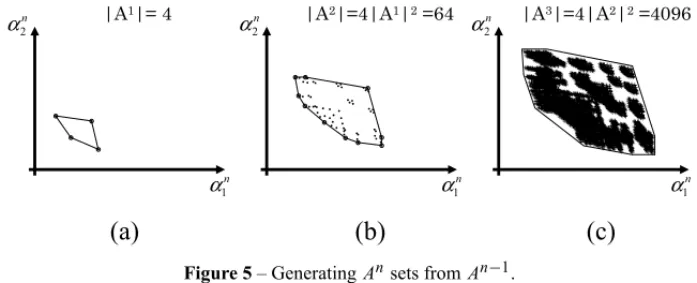
Theorem 1 provides the missing link to ensure that the value iteration algorithm is certain to arrive at the optimal solution for the finite-horizon problem and an arbitrarily good approximation for the infinite horizon problem in a finite amount of time. Unfortunately, this finite amount of time can be very large and often impractical. The difficulty lies in the efficient computation of the sets An since the size of these sets grows very fast with each step of the value iteration algorithm. In each iteration of the algorithm there is one newαvector for each possible product recommendation X for each permutation of size 2 of the vectors inAn−1. Consequently,|An| = |X|2n−1.
2
α
1
α
2
α α2
1
α α1
(a)
(b)
(c)
Figure 5– GeneratingAnsets fromAn−1.
this property is shared by all partially observable Markov Decision Problems (POMDPs), and the important developments in the literature have generated methods to (i) make the sets An as small as possible so as to minimize the size of An+1or (ii) find ways of quickly generating the sets Anfrom sets An−1. Sondik (1978) made significant theoretical contributions to the under-standing of the POMDP model and described the first algorithm for finding the optimal solution. Monahan (1982) formulated a linear program that finds the smallest possible setAnthat contains all the vectors a used in the optimal solution. Littman’s (1994) Witness algorithm is one of the most important contributions to the generation of An fromAn−1. Applications in robot naviga-tion resulted in a recent increase of interest in POMDPs in the artificial intelligence community (e.g., Kaelblinget al., 1996) which led to very important contributions in computational meth-ods. Littmanet al. (1995), for example, describe methods to solve POMDPs with up to nearly one hundred states. Tobin (2008) and Rosset al. (2008) provide a recent review of the state of the art in this field.
Figure 6 illustrates the results of numerical studies comparing the optimal policyμ∗, defined in (6) and computed using the Witness algorithm, and the myopic policyμM, which satisfies
μM(b)=arg max X∈X
n ˜
R(b,X)o. (12)
(a)
(b)
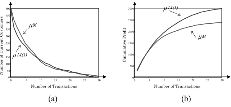
These results were obtained from simulations where companies started out with the same number of customers and gained no new customers over time. The graphs are typical of simulations done with varying numbers of customer segments and products. Graph 5(a) shows that the myopic policy is more likely to generate profits in the short-run, while the optimal policy does better in the long-run. The agent that acts optimally sacrifices sales in the beginning to learn about the customers to serve them better in the future. Graph 5(b) shows the cost of learning in terms of the customer base. The optimal policy leads to more customer defections due to low utility in the short-run, but the customers who stay receive consistently high utility in later periods and defect at much slower rates than customers being served by a myopic agent.
In spite of significant recent advances in computational methods, the optimal policy cannot al-ways be computed in a reasonable amount of time. Hence the need for approximate solution methods that produce good policies in an efficient manner. IfV∗(b)can be approximated by
˜
V(b), then the corresponding policyμ (˜ b)satisfies
˜
μ=arg max X∈X
( ˜
R(b,X)+γX
θ∈2
P(θ|b,X)V˜ (ϕ (b, θ ,X)) )
. (13)
There are several ways to approximating V∗(b). Bertsekas (1995b) discusses traditional ap-proaches, and Bertsekas & Tsitsiklis (1996) suggest alternative methods based on neural net-works and simulations. The paragraphs that follow describe the Limited Learning (L L) ap-proximation. This approximation is of interest because its corresponding customization policy yields good results and can be stated in simple terms which give insights into relevant managerial settings.
Limited learning policies are derived by assuming that the agent will stop learning after a fixed number of interactions. This restriction in the agent’s actions implies that the same product will always be recommended after a given point. These approximations are very good in situations where most of the learning occurs in the early stages.
Proposition 2 derives an expression for the policyμL L(b), which maximizes profits when agents are not allowed to change their beliefs between interactions.
Proposition 2.If agents are constrained to recommend the same product in all interactions with customers, then the infinite-horizon value function is given by
VL L(b)=max X∈X
|S| X
i=1
bi∙
piA(X) 1−γ 1−piL(X)
!
. (14)
and the corresponding policy by
μL L(b)=arg max X∈X
|S| X
i=1
bi∙
piA(X) 1−γ 1−piL(X)
!
Proof. See Appendix A.2.
TheμL L(b)policy can be re-written as
μL L(b)=arg max X∈X
n
b′∙3 (X)∙pA(X)o
where 3 (X)is a diagonal matrix that can be interpreted as the inverse of the risk associated with each recommendation for each segment. There are many ways to choose the elements of 3 (X). In the particular case of (18), the risk is fully captured by the probability of leaving. In a real world application, this would be an appropriate place to incorporate the knowledge of managers into the control problem. If all the diagonal elements of 3 (X)are the same, μL L reduces to the myopic policy. The matrix3 (X)scales the terms piA(X)by a risk factor unique to each product/segment combination. Therefore, under μL L products that are very good (or very safe) for only a few segments are more likely to be chosen than products that are average for all segments. The opposite would be true with the myopic policy. Consequently, agents acting according toμL L observe more extreme reactions and learn faster.
TheμL L(b)policy can be improved upon by allowing the agent to learn between interactions. In other words, the agent acts according toμL L(b)but updates the beliefs after each interaction. This idea can be generalized to a class of policies where during each period the agent solves a
n- period problem and chooses the action that is optimal for the first period, in a rolling-horizon manner. More precisely,
μL L(n) = arg max X∈X
( E
n X
t=0 γtrt
!)
s.t.
rn(b) = VL L(b)
In the specific case wheren=1 the corresponding policy is given by
μL L(1)=arg max X∈X
( ˜
R(b,X)+γX
θ∈2
P(θ|b,X)VL L(ϕ (b, θ ,X)) )
. (16)
(a)
(b)
0 5 10 15 20 25 30
0 50 100 150 200 250 300 350 400 450 500
0 5 10 15 20 25 30
0 500 1000 1500 2000 2500 3000 µ µ µ µ
Figure 7– Comparison of the “limited learning” and “myopic” policies.
The policyμL L(N)consistently yields good results in empirical tests. The expression forVL L(b) can be combined with an upper bound based on the assumption of perfect information to compute performance bounds as a function of the belief state:
max X∈X
|S|
X i=1
bi∙
piA(X)
1−γ1−piL(X)
≤V∗(b)≤
|S|
X i=1
bi∙max X∈X
piA(X)
1−γ1−piL(X)
. (17)
Note, first of all, that the upper and lower bounds are very close to each other in the extreme points of the belief space. The worst-case scenario happens when the company knows very little about the customer. In this case, however, we would expect the upper bound to be very loose, since it is based on the assumption of perfect information. This suggests that using the lower bound value function as a basis for control may yield good results even if the upper and lower bounds are not very close.
Figure 8– Possible configurations of customer segments and products.
We conclude this section listing five important properties of theμL L(1)policy.
1. Convergence to the optimal policy
As the belief state approaches the extreme points of the belief space, the upper and lower bounds are very close to each other. This implies that over time, as the company learns about the cus-tomer, the policyμ(L L)(b)will be the same as the optimal policy.
2. Lower the probability that the customer will leave after each interaction due to a bad recom-mendation.
This can only be guaranteed probabilistically because the observation error could theoretically be large enough to cause the customer to behave suboptimally. The likelihood of this event happening decreases as the utility of the recommendation increases, and the utility of the recom-mendations will increase over time.
3. Better revenues than the myopic policy.
When the company already knows the customer well,μL L(1)the myopic policy, and the optimal policy perform equally well. In situations where tthe agent needs to learn,μL L(1) loses to the myopic policy in terms of short-run revenue, wins in terms of expected revenues over time.
4. Learn faster than the myopic policy.
The myopic policy is more likely to suggest products that have similar utilities across all customer segments when the agent is not sure about the customer’s true segment. This situation is likely to happen at the beginning of the relationship, and suggesting such products leads to little, if any, learning.
5. Ease of computation (or, better yet, closed-form solution).
4 DISCUSSION
4.1 Solving of the Agent’s Dilemma
The main question of this paper is how companies should customize their products and services in settings such as the Internet. The analysis unambiguously shows that the pre-dominant paradigm of maximizing the expected utility of the current transaction is not the best strategy. Optimal policies must take into account future profits and balance the value of learning with the risk of losing the customer. This paper describes two ways of obtaining good recommendation policies: (i) applying POMDP algorithms to compute the exact optimal solution, (ii) approximating the optimal value function. The heuristic we provide worked well on the tests we performed, but we do not claim this heuristic to be the best one for all possible applications. Indeed, there are better heuristics for the solution of POMDPs with certain characteristics and the development of such heuristics for specific managerial settings is a topic of great interest to current researchers. The bounds analyzed in the previous section make explicit why agents acting according to a myopic policy perform so poorly. These agents fail to recommend products that can be highly rewarding for some segments because they fear the negative impact that these recommendations could have on other segments. This fear is legitimate – companies can lose sales and customers can defect – but it can be quantified through a matrix 3(X)that captures the risk associated with each possible recommendation for each segment. Optimally-behaving agents make riskier suggestions than myopic agents, learn faster, and earn higher payoffs in the long-run.
4.2 Learning and the Value of Loyalty
The more quality (utility) a company provides the customer, the more likely the customer is to come back. The better the company knows the customer, the more quality it can provide. Yet, learning about the customer can mean providing disutility (less quality) in the short-run. The in-teraction policy described in this paper reconciles these two apparently contradictory statements. The model suggests that the concept of loyalty must be expanded to incorporate learning. The extent to which repeated purchases lead to high value and loyalty depends on the company’s ability to learn about their customers as they interact.
The benefits of loyalty to profitability have been abundantly discussed in the managerial litera-ture. Reichheld (1996) gives the following examples of how loyalty leads to profits:
• In an industrial laundry service, loyal customers were more profitable because drivers knew shortcuts that made delivery routes shorter and led to cost reductions.
• In auto-service, if the company knows a customer’s car, it has a better idea of the type of problem the car will have and will be able to identify and fix the problem more efficiently.
These examples suggest an intimate relationship between learning and loyalty. In the laundry example, the fact that the customers have made a number of purchases from the same service provider has no direct effect on cost reduction. If a particular customer were to leave the company and its neighbor became a new customer, the cost savings would be the same in spite of the newness of the new customer. What seems to matter is knowledge, not length of tenure or number of previous purchases. Changes in profitability and retention rate over time depend on the firm’s ability to learn from past interactions and customize its services so as to provide customers with more quality.
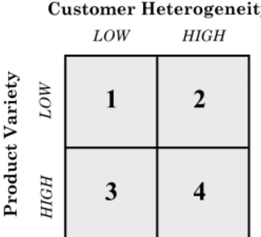
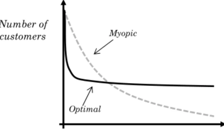
The observations of the previous paragraph are corroborated by the analysis of Section 3. Fig-ure 9 reproduces and labels the graph of FigFig-ure 6b. When the curves intersect, both firms have a customer base of sizeN who have been customers forT interactions. Even though both cus-tomer bases might be assigned the same value by a number of metrics (e.g., size of customer base, length of tenure) the difference in knowledge acquired during the first T interactions makes an enourmous difference in future profits. A metric such as RFM (recency, frequency, monetary value) might even assign a higher value to customers of the myopic agent. The ability to offer a large variety of products to a heterogeneous customer population (cell 4 in Figure 8) is not suffi-cient to generate rising revenues over time. It is also necessary to learn over time and customize services accordingly. Reinartz & Kumar (2000) make no mention of learning about customer preferences and customized services in their study, and their conclusion is that profitability per customer does not increase over time. Reichheld & Schefter (2000) conduct their study in the context of the Internet, where customer information is easily gathered and customization is com-monplace. Not surprisingly, they find that profits per customer rapidly increase over time and that the benefits of loyalty on the online world far exceed those of the brick-and-mortar world.
Figure 9– The effect of knowledge of profits.
4.3 The Value of Knowing the Customer
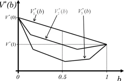
Consider, for example, a company operating in an industry where customers of Segment 1 are half as profitable as customers in Segment 2. Which marketing campaign would be most prof-itable: (i) one that only brings in customers from Segment 1 or (ii) one that brings customers from both segments with equal probability? The answer is that it depends on the shape of the value function. Figure 10 shows three possible value functions. IfV∗(b)=V1∗(b), then campaign (ii) is better; ifV∗(b)=V3∗(b), then campaign (i) is better. Both campaigns are equally profitable ifV∗(b)= V2∗(b). The intuition behind this result is that sometimes it can be costly to learn about one’s own customers. In some situations the company is better off knowing for sure that they are providing excellent value to the least desirable segment. The lower the switching cost and the higher the variance in the utility observation error, the more companies should invest in targeted advertising. This result provides an important connection between a firm’s acquisition and retention policies: theVi∗curves, which guide the acquisition policy, are determined by the customization policy.
) 0 ( *
) 1 ( *
) (
*
1 ( )
*
2 ( )
* 3
Figure 10– The value of customers as a function of how well the company knows them.
The more a company knows the preferences of a particular customer, the more it should want to learn even more about that customer in order to transform knowledge into cus-tomized, highly valued services. Intuitively, one may think the information is most valuable when the company doesn’t know anything about the customer. The convexity of the value function implies the opposite. In qualitative terms, the change in the value of the customer as the company’s level of knowledge changes from “very good” to “excellent” is greater than the change in value as knowledge goes from “average” to “good”. This finding provides a theoretical justification for the empirical finding that the difference in loyalty between “very satisfied” and “satisfied” customers is much greater than the difference between “satisfied” and “slightly dissatisfied” customers (e.g., Heskettet al., 1994). If a company knows a customer well, that customer will receive consistently good recommendations and be very satisfied.
5 DIRECTIONS FOR FUTURE RESEARCH
Management Science perspective, the issue of the best way to implement web-based customiza-tion policies remains open. The value funccustomiza-tion approximacustomiza-tions derived in this paper lead to a number of insights, but exact numerical methods generate better control policies. More work needs to be done to understand which approximation methods work best in situations where the problem is too large to compute the optimal policy. A second open question is how to recom-mend sets of products. In some situations agents are asked to recomrecom-mend more than one product. One obvious way of addressing this issue is to consider each possible set as a single product and reduce the problem to the one solved in this paper. This method can be inefficient if the set of possible products is large, because of the exponential increase in the number of potential sugges-tions. Therefore, it is worthwhile to explore other ways to generate good policies.
From the Consumer Behavior perspective, there are two topics of interest. First, the de-velopment of efficient perception management devices to reduce the probability of defection. In some situa-tions, it may be possible to have a “suggestion” to explore tastes as well as a “recommendation” to maximize utility. It has been shown that customers do not forgive bad recommendations, but could they forgive bad suggestions? Second, it is important to investigate how customers ag-gregate their experiences with agents over time. The model in this paper assumes that customer behavior is solely determined by the current product offering. In reality, the customers’ percep-tions of the agent’s quality evolve over time. But how exactly does this evolution take place? On one hand, there is a stream of research which suggests that recency (the satisfaction derived in the last few interactions) is the most important determinant of current satisfaction (for a review see Ariely & Carmon, 2000). On the other hand, first impressions are important and it can be very difficult for a customer to change his or her initial perception of the agent’s quality (e.g., Hogarth & Einhorn, 1992). These two views are in direct opposition, and it is not clear which is more important in web-based settings. Further research should also investigate how customers’ expectations change as a function of the quality of the advice they receive.
REFERENCES
[1] ARIELYD & CARMONZ. 2000. Gestalt characteristics of experienced profiles.Journal of Behavioral Decision Making,13: 219–232.
[2] ARIELY D, LYNCH JG & APARICIO M. 2004. Learning by collaborative and individual-based recommendation agents.Journal of Consumer Psychology,14(1&2): 81–94.
[3] BERGERPD & NASRNI. 1998. Customer lifetime value: Marketing models and applications. Jour-nal of Interactive Marketing,12: 17–30, (Winter).
[4] BERTSEKASD. 1995. Dynamic Programming and Optimal Control, Volume 1. Athena Scientific.
[5] BERTSEKASD. 1995. Dynamic Programming and Optimal Control, Volume 2. Athena Scientific.
[6] BERTSEKASD & TSITSIKLISJ. 1996. Neuro-Dynamic Programming. Athena Scientific, Belmont, MA.
[7] DONEYPM & CANNONJP. 1997. An examination of the nature of trust in buyer-seller relationships.
Journal of Marketing,61: 35–51, (April).
[9] HESKETTJL, JONESTO, LOVEMANGW, SASSERWE JR& SCHLESINGERLA. 1994. Putting the service-profit chain to work. Harvard Business Review. March-April, 164–174.
[10] HOGARTHRM & EINHORNHJ. 1992. Order effects in belief updating: The belief adjustment model.
Cognitive Psychology,24: 1–55, (January).
[11] JAIND & SINGH SS. 2002. Customer lifetime value research in marketing: A review and future directions.Journal of Interactive Marketing,16(2): 34–46.
[12] KAELBLINGLP, LITTMANML & MOOREAW. 1996. Reinforcement learning: A survey.Journal of Artificial Intelligence,4: 237–285.
[13] KOLLOCK P. 1999. The production of trust in online markets.Advances in Group Processes, 16: 99–123.
[14] LEWICKIRJ, MCALLISTERDJ & BIESRJ. 1998. Trust and distrust: New relationships and reali-ties.Academy of Management Review,23, (July).
[15] LITTMAN ML. 1994. The witness algorithm: Solving partially observable markov decision pro-cesses. Department of computer science, technical report, Brown University, Providence, R.I.
[16] LITTMAN ML, CASSANDRAAR & KAEBLINGLP. 1995. Learning policies for partially observ-able environments: Scaling up. In: PRIEDITISA & RUSSELLS (Eds), Proceedings of the Twelfth International Conference on Machine Learning, 362–370. Morgan Kaufmann, San Francisco, CA.
[17] MAESP. 1995. Intelligent software.Scientific American,273(9): 84–86.
[18] MCFADDEND. 1981. Econometric models of probabilistic choice. In: Structural Analysis of Discrete Data with Econometric Applications, MANSKYCF & MCFADDEND (Eds), MIT Press.
[19] MEYER RJ & KAHNBE. 1990. Probabilistic models of consumer choice behavior. Handbook of Consumer Theory and Research, ROBERTSONT & KASSARJIANH (Eds), Prentice-Hall.
[20] MONAHANG. 1982. A survey of partially observable markov decision processes: Theory, models, and algorithms.Management Science,28(1): 1–15.
[21] PFEIFERPE & CARRAWAYRI. 2000. Modeling customer relationships as Markov chains.Journal of Interactive Marketing,12(2): 43–55.
[22] REICHHELDF. 1996. The Loyalty Effect. Harvard Business School Press.
[23] REICHHELDF & SCHEFTERP. 2000. E- loyalty: Your secret weapon on the web.Harvard Business Review,78: 105–113, (July-August).
[24] REINARZ WJ & KUMAR V. 2000. On the profitability of long lifetime customers: An empirical investigation and implications for marketing.Journal of Marketing,64: 17–35.
[25] ROSSS, PINEAUJ, PAQUETS & CHAIB-DRAAB. 2008. Online Planning Algorithms for POMDPs.
Journal of Artificial Intelligence Research,32: 663–704.
[26] ROSSIP, MCCULLOCHR & ALLENBYG. 1996. The value of purchase history data in target mar-keting.Marketing Science,15(4): 321–340.
[27] SONDIKEJ. 1978. The optimal control of a partially observable markov decision process over the infinite horizon: Discounted costs.Operations Research,26: 282–304.
[29] TOUBIAO, SIMESTER DR & HAUSER JR. 2003. Fast polyhedral adaptive conjoint estimation.
Marketing Science,22(3): 273–303.
[30] URBAN GL, SULTANF & QUALLSWJ. 2000. Placing trust at the center of your internet strategy.
Sloan Management Review,42(1): 39–48.
[31] WHITE III CC. 1976. Optimal diagnostic questionnaires which allow less than truthful responses.
Information and Control,32: 61–74.
[32] ZAUBERMANG. 2000. Consumer choice over time: The perpetuated impact of search costs on deci-sion processes in information abundant environments. Ph.D. Dissertation, Duke University, Durham,
NC.
A Appendix
A.1 Proof of Proposition 1
The proof is by induction, and therefore consists of the verification of a base case and the induc-tion step.
(1) Base case: To prove that there exists a set of vectors A1 such that V1(b)=max
α∈A1(b∙α) .
The optimal policy with 1 step to go is to act myopically with respect to immediate payoffs:
V1(b)=max X∈X
n ˜
R(b,X)o=max
α∈A1(b∙α)
where the last equality holds by letting A1= S X∈X
piA(X) .
(2) Induction step
If
∃An−1such thatVn−1(b)= max
α∈An−1(b∙α)
then
∃Ansuch thatVn(b)=max
α∈An(b∙α)
From the induction hypothesis, we can write, forθ∈
θA, θR ,
Vn−1(ϕ (b, θ ,X))= max
α∈An−1(ϕ (b, θ ,X)∙α)=ϕ (b, θ ,X)∙α
n−1(
b, θ ,X) (18)
where
αn−1(b, θ ,X)=arg max
α∈An−1
(ϕ (b, θ ,X)∙α) .
SinceVn =T Vn−1, we obtainVn(b)by applying the mapping(T V) (b)to theVn−1function above:
Vn(b)=max X∈X
˜
R(b,X)+γ X
θ∈
θA,θR
Pr(θ|b,X) h
ϕ (b, θ ,X)∙αn−1(b, θ ,X) i
Recall the definition ofϕ (b, θ ,X)and note thatϕ b, θA,X
andϕ b, θR,X
can be written as
ϕb, θA,X= b∙Ŵ
A(X) Pr θA|b,X
and
ϕb, θR,X= b∙Ŵ
R(X) Pr θR|b,X.
If we substituteR˜(b,X)= |S| P
i=1
bi∙R Si,Xj
and the expressions forϕ (b, θ ,X)above into the expression forVn(b)we obtain
Vn(b)=max X∈X
b∙ pA(X)+γ∙b∙ŴA(X)∙αn−1
b, θA,X
+γ∙b∙ŴR(X)∙αn−1b, θR,X
by cancelling out the terms Pr θA|b,X
and Pr θR|b,X .
Factoring out the vectorband defining the setAnas
An= [
X∈X
[
αi∈An−1
[
αj∈An−1
pA(X)+γ ŴA(X)∙αi+γ ŴR(X)∙αj
we conclude that
Vn(b)=max
α∈An(b∙α)
A.2 Proof of Proposition 2
If agents are not allowed to learn, then the value function that maximizes future expected profits for then−period problem is given by
ˆ
Vn(b)=max
α∈ ˜An
(b∙α) .
whereAˆ1= A1and the sequence of setsnAˆ1,Aˆ2, ...,Aˆnois defined by the recursion
ˆ An= [
X∈X
[
αi∈ ˆAn
h
pA(X)+Ŵ(X)∙αii
whereŴ (X)=ŴA(X)+ŴR(X).
The value functionsVˆn(b)can be explicitly written as maximizations overα∈ ˆA1as follows:
ˆ
V1(b) = max
α∈ ˆA1
(b∙α)=max X∈X
ˆ
V2(b) = max
α∈ ˆA2
(b∙α)=max X∈X
b∙hpA(X)+Ŵ (X)∙pA(X)i
.. .
ˆ
Vn(b) = max
α∈ ˆAn
(b∙α)
= max X∈X
b∙hpA(X)+Ŵ (X)hpA(X)+Ŵ (X)[pA(X)+ ∙ ∙ ∙i∙ ∙ ∙i∙pA(X)
= max X∈Xb∙p
A(
X)+b∙Ŵ (X)∙pA(X)+ ∙ ∙ ∙ +b∙[Ŵ (X)]n−1∙pA(X)
= max X∈Xb
" I+
n−1 X
i=1
[Ŵ (X)]i #
∙pA(X)
The sequence of functionsVˆn(b)converges:
lim n→∞
ˆ
Vn+1(b)− ˆVn(b)= (20)
= lim
n→∞ maxX∈Xb
" I+
n−1 X
i=1
[Ŵ (X)]i #
∙pA(X)−max X∈Xb
" I+
n−2 X
i=1
[Ŵ (X)]i #
∙pA(X) !
= lim n→∞
max
X∈X[Ŵ (X)]
n∙pA(X)
= 0
The last step follows from the fact that all the elements in Ŵ (X)are in (0,1), and therefore lim
n→∞[Ŵ (X)]
nis a matrix of zeroes. Now consider the difference
Dn(b)=b∙ ˆα−Vn(b)
where
ˆ
α=arg max X∈X
b∙[I−Ŵ (X)]−1∙hpA(X) i
.
Substituting the full expression forVn(b)yields
Dn(b)=max X∈X
b∙[I−Ŵ (X)]−1∙hpA(X)i− max X∈Xb∙
" I+
n−1 X
i=1
[Ŵ (X)]i #
∙pA(X) !
Since all the elements ofŴ (X)are in(0,1), the expression [I−Ŵ (X)]−1 is well-defined and can be expanded to
[I−Ŵ (X)]−1=I+ ∞ X
i=1
Substituting the expansion above into the expression forDnyields
Dn(b)=max X∈X b∙
" ∞ X
i=n
[Ŵ (X)]i #
∙pA(X) !
.
It then follows that
lim n→∞D
n(b)=0,∀b (21)
The result from (20) ensures that the sequence Vn(b)converges to a limit V∗(b). Equation (21) asserts thatVn(b)also converges tob∙ ˆα.Since the dynamic programming mapping is a monotone contraction, the limit is unique, so αˆ corresponds to the policy that maximizes the infinite horizon value function.
A.3 Simulation parameters
Parameters used for simulation in Figure 7:
c=2.5
ε∼N or mal(0,3)
u1(1)= −2 u2(1)=5
u1(2)=5 u2(2)= −2
u1(3)=0 u2(3)=0