A General Boundary Condition with Linear Flux
for Advection-Diffusion Models
†T.Y. MIYAOKA1*, J.F.C.A. MEYER1 and J.M.R. SOUZA2
Received on November 21, 2016 / Accepted on April 19, 2017
ABSTRACT.Advection-diffusion equations are widely used in modeling a diverse range of problems. These mathematical models consist in a partial differential equation or system with initial and boundary conditions, which depend on the phenomena being studied. In the modeling, boundary conditions may be neglected and unnecessarily simplified, or even misunderstood, causing a model not to reflect the reality adequately, making qualitative and/or quantitative analyses more difficult. In this work we derive a general linear flux dependent boundary condition for advection-diffusion problems and show that it generates all possible boundary conditions, according to the outward flux on the boundary. This is done through an inte-gral formulation, analyzing the total mass of the system. We illustrate the exposed cases with applications willing to clarify their meanings. Numerical simulations, by means of the Finite Difference Method, are used in order to exemplify the different boundary conditions’ impact, making it possible to quantify the flux along the boundary. With qualitative and quantitative analysis, this work can be useful to researchers and students working on mathematical models with advection-diffusion equations.
Keywords: boundary conditions, partial differential equations, mathematical models, computer simula-tion.
1 INTRODUCTION
The first application of the diffusion equation was done by Fourier in 1822 [1], when he proposed its use to model heat distribution. At that time, the main concern was to analyze the model for simple cases, including simple boundary conditions such as fixed concentrations at the bound-aries. Once theory was developed, the diffusion equation can now be combined with advection (or convection) processes, resulting in advection-diffusion equations, which demand more elab-orate boundary conditions, depending on the phenomena being modeled.
†This work was supported by CAPES.
*Corresponding author: Tiago Yuzo Miyaoka – E-mail: [email protected]
1Departamento de Matem´atica Aplicada, IMECC, Universidade Estadual de Campinas, R. S´ergio Buarque de Holanda, 651, 13083-859 Campinas, SP, Brasil. E-mail: [email protected]
In [2], the authors separate the applications of advection-diffusion models in two categories: inorganic, such as temperature and concentration of matter, and organic, populations of organ-isms, which is the main concern of their book. Amongst other interesting and rich examples, the authors cite the applications to diffusion of spores, insect pheromones, insect dispersal. An application to temperature and heat transfer can be found in [3]. Advection-diffusion models have been widely used in mathematical ecology. Applications include organic subjects, as in [2], and inorganic, in a way inspired by that of [4], modeling pollution dispersal. The main purpose of these works is to obtain models based on advection-diffusion equations or systems and nu-merical approximations to their solutions, generally by means of the Finite Elements or Finite Differences methods. Some works analyzed pollutant dispersal, either in rivers [5], in the sea [6], lakes in two [7] and three dimensions [8], air [9], or mixed [10]. In [11], steady-state air pollution is modeled. Other works treated the diffusion of interacting animals, as the change of habitat in fish [12], biological control of the boll weevil [13], biological control of the horn fly affecting beef cattle [14], and skipjack tuna movement in the western Pacific Ocean [15]. Other works studied the diffusion of population dynamics in the presence of pollutants, as in a two preys system [16], two predators and two preys system [17], two competitors [18], development of macroalgae [19], and the sediment impact in four benthic populations [20]. A different approach is the consideration of diffusion and migration (advection) in epidemiological compartmental models, as a capybara disease [21], foot-and-mouth disease [22], and avian influenza [23]. Gen-eral population movement is also studied, aiming to compare different models and/or techniques, as in [24, 25, 26, 27]. As each of these works has their own particularities, appropriate analyses at the boundaries are necessary in each case, but in most of the cited cases, the authors decided to make simple assumptions in order to obtain more tractable boundary conditions, sometimes due to lack of information about the studied phenomenon. One exception is the already mentioned work [6], in which the authors consider a boundary condition similar (but less general) to the one treated in this present work. The inappropriate use of boundary conditions can lead to models which do not reflect reality so well, or to different interpretations, disturbing qualitative and/or quantitative analyses. For the interpretations, we will be based on the previously cited works, considering mostly the pollution case, but sometimes analogies using the animals and heat cases will help us understand the model as a whole.
A simple analysis about boundary conditions in ecological problems modeled by advection-diffusion equations can be found in [28], where the authors relate the outward flux with the concentration present on the boundary, but only for the homogeneous case. In the previously mentioned work [2], the authors consider boundary conditions for each specific model, lacking a general analysis. A derivation for flux conditions can be found in [29], but only for a specific application.
In Section 2, we derive a general boundary condition with linear flux for an advection-diffusion equation, through an integral formulation. Integrating the concentration under study over the spa-tial domain, we obtain the total mass of the system, to which the analyses are made, in each of its particular cases. In Section 3, numerical simulations with the Finite Difference Method are made and mass by time graphs are shown for several particular boundary conditions. Additionally, a convergence analysis for numerical errors is made. The discretization and a brief algorithm is shown in Appendix 4. Conclusions are presented in Section 4.
Considering an initial–boundary value problem inu = u(x,t), x = (x1, . . . ,xn) ∈ Rn, we have in literature [29] three different boundary condition types: Dirichlet, Neumann and Robin, each of these being separated in homogeneous, if it does not involve values beyondu, or non homogeneous, if it does. These conditions can be found in Table 1, whereuis the solution of the boundary value problem, f,g, andh are arbitrary functions anda andb arbitrary parameters, which may or may not depend on(x,t). A Dirichlet, or first kind, condition specifies the value of
uon the boundary, either being zero or any functionf that may depend or not on other variables. A Neumann, or second kind, condition, on the other hand, specifies the derivative of the solution
u along the boundary, more precisely the directional derivatives in the direction of the external unitary normal vectorn, as also shown in Table 1. A Robin, or third kind, condition involves both the value ofuand its derivative, specifying an equation that must be valid along the boundary, as in the last two rows of Table 1. In the next sections, we will consider only two spatial variables
(x,y), but all the analyses are analogous to one or three, or evenndimensional problems.
Table 1: Boundary Condition Types.
Condition Kind
u=0 homogeneous
Dirichlet or first kind
u= f(x,t) non homogeneous
∂u
∂n =0 homogeneous
Neumann or second kind
∂u
∂n =g(x,t) non homogeneous
au+b∂u
∂n =0 homogeneous
Robin or third kind
au+b∂u
∂n =h(x,t) non homogeneous
2 MATHEMATICAL MODELING OF BOUNDARY CONDITIONS
sources, among others, as in some of the previously cited works. Also consider a population of animals spreading in a territory, such as its natural habitat or a confined space, with some preference in its movement, which generates a transport effect, plus other possible influences such as vital dynamics. Both, substance and animals, can be modeled by the advection-diffusion equation [2, 28]:
∂u
∂t + ∇ ·(−α(x,y)∇u+V(x,y)u)= f(u,x,y,t). (2.1)
Whereu denotes the concentration of substance or animals, with mass/distance2 units; the∇ operator is calculated in spatial variables x and y; α(x,y) is the diffusion coefficient, with distance2/time units;V(x,y) = (v(x,y), w(x,y))is the velocity or migration field with dis-tance/time units; and f(u,x,y,t)is an external concentration source with mass/(distance2time) units, which includes reaction, dynamic terms, depending or not onu. For simplicity we will consider f identically null, as it does not alter the analyses on the boundary. A similar approach with f different from zero can be found in [29]. The spatial domain, the water medium or animal habitat, is an open bounded region∈R2with boundary∂and the temporal interval is given byI =(t0,tf]. Besides that,u(x,y,t0)=u0(x,y)is an arbitrary initial condition.
This problem can be simplified to a stationary one in a direct way, considering the temporal derivative as zero in (2.1). All boundary analyses are applicable to the stationary case in the same way as in the temporal one.
Another situation, where a temperature diffuses in a thin metal plate, with an external source of heat represented by f, can also be modeled by equation (2.1), but with the advection term null,
V(x,y)=0.
2.1 General Boundary Condition Derivation
In order to obtain the most general boundary condition to this equation, we integrate (2.1) over the whole domain, at an arbitrary time instantt ∈ I, already considering f(u,x,y,t)identically null:
∂u
∂t d A+
∇ ·(−α∇u+Vu)d A=0.
Consideringu(x,y,t)uniformly continuous int, we can take the temporal derivative out of the integral. Applying the Divergence Theorem to the second term, one obtains:
∂
∂t
u(x,y,t)d A+
∂
(−α∇u+Vu)· n ds=0. (2.2)
We observe that
u(x,y,t)d A=M(t), whereM(t)is the total mass ofuinside the domain
for eacht ∈ I. The equation (2.2) may then be written depending on the total mass variation rate:
d M(t)
dt +
∂
This way, if we want the total mass variation of the system to be null, i.e., that there is no incoming nor outgoing concentration in the domain, then the temporal derivative in (2.3) should
be null and:
∂
(−α∇u+Vu)· n ds=0.
The only way for this integral to be zero for any solutionu, is if the integrand itself is zero. This integrand is the outward normal component of the flux of the concentrationuover the domain,
J(u)= −α∇u+Vu. The term−α∇udenotes the flux due to diffusion andVu the flux due to
advection. Rearranging the terms, observing that∇u· nis the directional derivative ofu in the normal direction, the outward flux must be null, for(x,y)∈∂andt∈ I:
−α∂u
∂n +V· n u =0. (2.4)
This is the null flux boundary condition for (2.1). We wish to obtain a condition in which the exit/entrance flux is not zero, but dependent on factors external to the domain and/or concen-tration density on the boundary. For this purpose, we equal the flux at left hand side of (2.4) to a linear combination ofu and an external source, obtaining the following general linear flux boundary condition, for(x,y)∈∂andt ∈I:
−α∂u
∂n+V· n u=β(u−c)+γc. (2.5)
Wherec = c(x,y,t)represents an external source of concentration, such as f(u,x,y,t)but acting only on the boundary and independent ofu.βandγ are parameters, which might or not depend on(x,y)andt, and relate the entrance/exit rate of concentration on the boundary with
u andc densities. Bothβ andγ have distance/time units andchas mass/distance2 units. In this work we considerβ andγ as constants, and positive unless specified, for didactic purposes, but the extension is straightforward. The word “linear” means that the flux along the boundary depends linearly onu. Writing this condition in another way:
−α∂u
∂n+V· n u=βu+(γ −β)c. (2.6)
We can then see that the flux dependent onuis proportional toβ, while the external flux, due to
c, is proportional toγ−β. We may haveβ,γ, and/orc=0, each situation providing particular cases. Varying these combinations we have all possible boundary conditions with linear flux. The particular linear combination at the right hand side of (2.4) or (2.6) was carefully taken in order to model the fluxes of bothuand external sourcecalong the boundary, in a general point of view. Applications and examples are exhibited in the next sections.
To analyze the meaning of each term of the right hand side of condition (2.4) or (2.6), we return to the total mass system analysis, but this time imposing the generalized condition (2.5) directly upon equation (2.3), obtaining:
d M(t)
dt = −
∂
βu ds−
∂
γc ds+
∂
The line integrals in this equation represent u andc masses on the boundary of the domain. These masses are proportional to ratesβ andγ, which are influencing the total mass variation. Consideringβ > 0,γ > 0 andc> 0, we have escape of concentrationu with rateβ, escape of concentrationc with rateγ, and entrance of concentrationc with rateβ. This can be seen schematically in Figure 1. If the signs ofβ,γ orcwere exchanged, their entrances and escapes would need to be inverted.
βu
βc
γc
∂
Ω
Ω
Figure 1: Flux illustration for equation (2.1) with boundary condition (2.5). Ifβ >0, γ >0, andc>0, the fluxβuandγcare outward, while the fluxβcis inward.
For a better analysis of this condition, in the following we will divide it in distinct cases forβ, consideringβ → ∞,β =0, andβ =0,β < ∞, in each of these cases consideringγ,cand
Vnull or not. A summary can be found in Table 2. As previously said, these options covers all
possible boundary conditions with linear flux for equation (2.1).
2.2 Flux independent ofu,β =0
2.2.1 External source,γ =0andc=0
In this case we considerβ =0, i.e., we do not consider flux dependent uponu. So (2.5) turns into:
−α∂u
∂n +V· n u =γc. (2.7)
This non homogeneous Robin condition relates the flux with the external sourcecby means of the rateγ. In this case we have a constant, or at least not dependent onu, concentration removal in the system (or injection, ifγc<0).
An example could be withuas a pollution, andcacting by removing pollution on the boundary from inside to outside the domain, regardless of the quantityu that is already on the domain. Or, ifγc <0 so the flux is positive in the outward direction, it would be an external source of concentration from outside the boundary to inside the domain.
2.2.2 Null flux,γ =0and/orc=0
If eitherγorcare also null, we should have no external source:
−α∂u
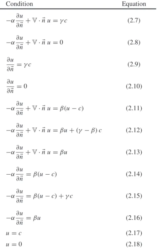
Table 2: Summary of boundary conditions for equation (2.1)
Condition Equation
−α∂u
∂n+V· n u=γc (2.7)
−α∂u
∂n+V· n u=0 (2.8)
∂u
∂n =γc (2.9)
∂u
∂n =0 (2.10)
−α∂u
∂n+V· n u=β(u−c) (2.11)
−α∂u
∂n+V· n u=βu+(γ −β)c (2.12)
−α∂u
∂n+V· n u=βu (2.13)
−α∂u
∂n =β(u−c) (2.14)
−α∂u
∂n =β(u−c)+γc (2.15)
−α∂u
∂n =βu (2.16)
u =c (2.17)
u =0 (2.18)
Which is the same homogeneous Robin condition as (2.4), with no flux and the total mass of the system constant, as discussed before. We can interpret this equation as an equality between the normal components of diffusion flux and advection flux, in order to maintain the concentration exchange null.
in which the value ofuis constant along the boundary, that is: everything that enters is equivalent to whatever leaves the domain, so that the flux is null.
2.2.3 External source with no advection,γ =0,c=0andV=0
In the particular case of the purely diffusive problem,V=0, and condition (2.7) simplifies to a
non homogeneous Neumann one:
−α∂u
∂n=γc. (2.9)
In the purely diffusive problem the flux is given solely by the directional derivative (Fick’s law [2]), so the interpretation is the same as of (2.7).
The pollutant case is also valid as an example here, not considering the transport by making
V=0. But another example can be the previously mentioned heat problem, withu measuring the temperature in a metal plate and at the boundaries a fixed temperature being kept by some external source. Consideringuas the ambient temperature, the domain could be a room isolated from outer temperature, with a heater inside, represented byc.
2.2.4 Null flux with no advection,γ =0orc=0andV=0
Ifγ =0 orc= 0 in the purely diffusive case, we have the following homogeneous Neumann condition, which is a particular case of (2.8):
∂u
∂n =0. (2.10)
Continuing with the temperature example, this condition means that the boundaries are perfectly isolated so that there is no influence of the external media to the inside temperature. This may occur in a metal plate or in the ambient temperature examples, without external influence.
We observe that this condition is a no flux one only for the purely diffusive case, and if applied to the general problem (2.1), it will neglect the advective fluxV· n u. This would mean that
βu = V· n u, withβ = 0, considering a flux due to βu that actually does not exist. This condition may be interesting if the boundary in study is a barrier to diffusion, so the diffusive flux will be null, but not a barrier to advection, leaving its flux unaltered.
2.3 Partial flux,β =0
2.3.1 Exchange between inside and outside,γ =0andc=0
Before proceeding to the general case, in which all the parameters in (2.5) are different from zero, we will consider the case in which onlyγ =0, i.e., only the rate due to external source is taken as zero. Then we have the following non homogeneous Robin condition:
−α∂u
This condition tells us that parameterβ relates the flux exchange, exit or entrance, of bothu and
con the boundary. That is, ifu >c, withβ > 0, then concentrationu along the boundary is greater than the external sourcec, therefore the flux is positive to the outside and this difference is balanced. Ifu < c, withβ > 0, then the external source is greater than the concentration on the boundary, and then the flux is negative as well as the sign ofβ (u−c), leading to an inward flux.
In the pollutant example, this condition models an exchange of concentration on the boundary, depending on both external concentration,c, and internal,u, as explained in the previous para-graph, as an osmosis phenomenon, greater concentrations tend to migrate to locations with lower concentrations. Consideringuas confined animals, this condition would mean that they can leave and enter along the boundary, not freely, but accordingly to the concentration present there. So the animals would leave the domain if the concentration were grater thanc, or enter if it were smaller thanc.
2.3.2 Dependence onuand external source,γ =0andc=0
This is the most important condition, because it includes all others. It is a non homogeneous Robin condition and arises when all the parameters in (2.5) are non zero. We rewrite it here in two different ways for convenience:
−α∂u
∂n+V· n u=βu+(γ −β)c. (2.12a)
−α∂u
∂n+V· n u=β (u−c)+γc. (2.12b)
Looking at (2.12a) we can divide the flux in two parts: one depending onu and the other onc. The greater the concentration ofu on the boundary, the greater will be the exit (or entrance) of it, beingβthe rate that regulates this change. Ifβ >0, we have entrance, and ifβ <0, we have exit ofu from the domain. Also, the flux relative to(γ −β)cdoes not vary withu, but it can depend onx,y,tifγ,βand/orcdo so. The sign ofγ−βtells us if there is input into (γ > β), or output from the domain (γ < β) of external sourcec.
On the other hand, looking at (2.12b), we can see that the termγc is a constant injection of concentration as in (2.7), which is related to factors external to the domain. Also, the termβ(u−
c)is the same as in (2.11), having here the same role. So we see thatβis a parameter that relates the inside of the domain to the outside, whileγ does not depend on the inside, considering only the contribution of external factors.
2.3.3 Dependence onu,γ =0andc=0
In the caseγ =β, orc=0, (2.11) becomes a homogeneous Robin condition:
−α∂u
∂n+V· n u=βu. (2.13)
This condition relates the flux only with the density along the boundary, without external factors. Ifβ > 0, this condition means that the flux is outward positive so, asu increases, the exit of concentration from the domain becomes higher. Ifβ < 0, we have the opposite. We note that this is a particular case of (2.11) without an external balance factor, so that the behavior of the flux does not depend on the outside of the domain.
An example could be either the pollutant or the animals case, in a boundary which allows passage, similar to that of (2.11) but without contributions from the outside. According to [28], this is the standard boundary condition for equation (2.1).
2.3.4 Dependence onu,γ =β,c=0
In this case, the condition also reduces to (2.13), but there is a conceptual difference: the external sourcecis not null, but the equality between the ratesγ andβcauses the whole term(γ −β)c
in (2.12a) to vanish, so that there is an equality between the entrance and exit ofcin the domain:
βc=γc(which is entrance or exit depends on the signs involved).
This situation is highly unlikely because the model is an approximation of the reality, therefore parameters considered do not have precise values. A possible example could be, in the pollutant case, an artificial regulation of γ, in order to precisely cause the equalityγ = β, if one can control the entrance/exit of the pollutant.
2.3.5 Exchange between inside and outside with no advection,γ =0,c=0andV=0
Considering now the purely diffusive case,V=0, andγ =0, we have:
−α∂u
∂n =β(u−c), (2.14)
with same interpretation as in (2.11). The example in (2.11) about the pollutant is also valid here, but a typical example is the temperature case, this condition being known as the heat radiation boundary [3], where there is heat exchange with the external media. In this fashion,crepresents the external temperature, and the boundary condition balances the difference in the temperature from inside the domain and outside, with the same analysis as in (2.11).
2.3.6 Dependence onuand external source with no advection,γ =0,c=0andV=0
In the purely diffusive case,V=0, the general linear condition is:
−α∂u
which is a particular case of (2.12), just without the advection term, so the same interpretation is valid. Again consideringuas the ambient temperature in a room, this combines the radiation boundary in (2.14) and the external source in (2.9), so that there is an exchange of temperature with the exterior of the room and an internal source of heat.
2.3.7 Dependence onuwith no advection,γ =0orc=0andV=0
If, besidesV=0, eitherγ =0 orc=0, we have an homogeneous Robin condition:
−α∂u
∂n =βu, (2.16)
which is a particular case of (2.13).
In the heat diffusing in a metal plate, this means that there is change of temperature in the ex-tremes of the plate, which does not depend on the outside, but only on the temperature along the boundary.
2.4 Total flux,β→ ∞
2.4.1 Total flux with external source,c=0
Rewriting condition (2.5) in order to isolateu−c, we obtain:
1
β
−α∂u
∂n+V· n u−γc
=u−c.
Increasing the flow due to the presence ofuin the boundary indefinitely, i.e. considering unlim-ited growth ofβ, so thatβ → ∞, we have the following non homogeneous Dirichlet condition:
u =c. (2.17)
This tells us that all concentrationuthat arrives on the boundary dissipates, because the flux due toβ is unlimited, thereby the value ofu is completely described by the external sourcec.
In the pollution example, the unlimited growth ofβ means that all the pollution arriving on the boundary crosses it completely, or is totally absorbed, so that the only concentration of pollutant that remains there is due to the external sourcec.
2.4.2 Total flux without external source,c=0
If besidesβ → ∞we also havec=0, we obtain the homogeneous Dirichlet condition, which also has total exit flux but without external source, keeping the concentration zero along the boundary:
In the pollution case, we also have a complete passage of concentration, but without any source, so that the concentration remains zero on the boundary. In a population dispersal case, this con-dition can be used in a situation in which no animal can stay along the boundary, because of the terrain, for example.
We note that the same conditions, (2.17) or (2.18) are valid ifα = 0,V =0, or evenγ =0, thereby the total flux condition is independent of these quantities.
2.5 Mixed boundary conditions
In practical situations, mathematical models often consider domains with heterogeneous bound-aries. This means that the boundary∂must be separated in several regions∂i,i=1, . . . ,N,
with∂= ∪N
i=1∂i, the union being disjoint. Each of these regions∂i can then be modeled by any of the presented boundary conditions (2.7)–(2.18). Most of the already mentioned works utilize this kind of mixed boundary conditions in their models. In particular, in [10] the authors explain each part of the boundary considered for an air/lake pollution model.
3 NUMERICAL SIMULATIONS
In order to obtain numerical approximations to solutions of problem (2.1), we utilized second order Finite Difference formulas in spatial variables and Crank–Nicolson Method in the time variable [30]. For simplicity we considered a rectangular domain = [0,L] × [0,H]. For boundary points we applied the finite difference formulas directly in the boundary conditions obtaining complementary equations. We then obtained an algebraic linear system to be solved at each time step, which is solved by theLUfactorization method. As the system matrix is constant, it may be factorized only once. Matlab was used for the implementation of the computational routines. Details about the numerical solutions calculations can be found in the Appendix.
The illustrative parameters utilized wereα=0.1;V=(0.02,0.02);β =0,β =0.1,β=0.05, or β = 100; γ = 0, γ = 0.1 or γ = 0.05; c = 0, c = 1 orc = −1. The length and height of the domain were L = H = 1, and the time interval J = (0,2]. The domain was discretized using 26intervals in bothxandydirection and 210in time. The initial condition was
u0(x,y)=κexp(−64((x−0.5)2+(y−0.5)2)), a gaussian at the center of the domain, where
κis a constant to maintain initial mass equal to the unit. This gaussian was chosen because it has negligible value on the boundary of the domain. Therefore at the beginning of the simulations, the boundary is unaffected. As one can obtain any of the exposed boundary conditions from (2.5), this general expression was used in the implementation, and the parameters adjusted to obtain the different conditions.
(a) β=0,γ =0.05,c=1 (b)β=0,γ =0.05,c= −1 (c)β=0,γ=0,c=0
(d)β=0.1,γ=0,c=1 (e)β=0.05,γ=0.1,c=1 (f)β=0.1,γ=0.05,c=1
(g)β=0.1,γ=0,c=0 (h)β=100,γ =0,c=1 (i)β=100,γ =0,c=0
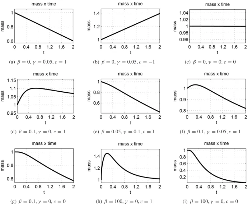
Figure 2: Mass by time graphs in numerical solutions of problem (2.1), for boundary condi-tions (2.7): 2(a), 2(b), (2.8): 2(c), (2.11): 2(d), (2.12): 2(e), 2(f), (2.13): 2(g), (2.17): 2(h), and (2.18): 2(i).
The non-simulated conditions are particular cases from these but for the purely diffusive case, so that their analyses are the same.
In Figure 2(a) the parameters wereβ =0,γ =0.05, andc=1. We have condition (2.7) with
γc>0, which implies in outward linear flux along the boundary. The flux is constant, given by
γc, therefore the mass decreases linearly.
In Figure 2(b) the parameters wereβ = 0,γ = 0.05,c = −1. We have condition (2.7) with
γc<0, which implies in inward linear flux on the boundary. The flux is constant, therefore the mass increases linearly.
In Figure 2(d) the parameters were β = 0.1,γ = 0, c = 1. We have condition (2.11), with exchange between internal and external concentration, given by u and crespectively. At the beginning there is inward flux, because u < con the boundary, therefore the mass increases. But after (approximately att =0.6), the flux becomes outward, as the concentration along the boundary increases makingu>c, and the mass decreases.
In Figure 2(e) the parameters wereβ =0.05,γ =0.1,c=1. We have condition (2.12), with the combined effects of (a) and (d). Therefore the flux is always outward because of the termγc, but it starts small and increases because ofβ(u−c). The mass always decreases.
In Figure 2(f) the parameters wereβ =0.1, γ = 0.05,c = 1. We have condition (2.12), but withβ < γ, therefore the flux due tocin inward, causing the concentration to increase at the beginning. As the system mass increases, so does the termβu, and the flux becomes outward (approximately att =0.3), causing the mass to decrease.
In Figure 2(g) the parameters wereβ =0.1,γ =0,c=0. We have condition (2.13), with flux dependent only onu. As in the very beginning there is no concentration on the boundary, the mass remains constant. But as concentration increases along the boundary, so does the outward flux, causing the mass to decrease.
In Figure 2(h) the parameters wereβ =100,γ =0,c=1. We have condition (2.17), with total flux is outward the domain, and also a total injection due toc. At the beginning there is an increase in the mass, because there is only injection. Afterwards there is a decrease in concentration due to the total outward flux.
In Figure 2(i) the parameters wereβ =100,γ =0,c=0. We have condition (2.18), with total flux outward and no external source. The flux becomes higher as the concentration starts to cross the boundary causing the mass to decrease.
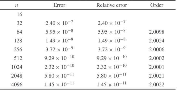
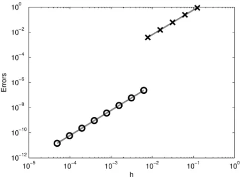
In Tables 3 and 4 we show convergence tests for our numerical solutions. In each table we show absolute and relative errors in max norm obtained comparing solutions in consecutive meshes, which consist in regular subdivisions of the domain. In Table 3,ndenotes the number of divisions inxandydirections, which are equal, and in Table 4,nis the number of divisions in timet. For the temporal convergence, we used the mass of the system M(t)for the errors, which contains information of the whole spatial domain. We also show the numerical rate of convergence of the methods comparing two consecutive errors. As expected, both in space and time the rates obtained converge to 2, since the methods used havex2,y2andt2orders. In Figure 3 we show an error by mesh grid sizes loglog graph for both spatial and temporal analyses, with linear fits for each case. These results collaborate to the accuracy of the results obtained.
4 CONCLUSION
Table 3: Spatial errors and rates of convergence for (2.1) numerical solutions.
n Error Relative error Order
8
16 8.86×10⁻¹ 5.35×10⁻²
32 2.45×10⁻¹ 1.50×10⁻² 1.8565 64 6.16×10⁻² 3.79×10⁻³ 1.9889
128 1.54×10⁻² 9.50×10⁻⁴ 1.9988
256 3.86×10⁻³ 2.38×10⁻⁴ 1.9998
Table 4: Temporal errors and rates of convergence for (2.1) numerical solutions.
n Error Relative error Order
16
32 2.40×10⁻⁷ 2.40×10⁻⁷
64 5.95×10⁻⁸ 5.95×10⁻⁸ 2.0098
128 1.49×10⁻⁸ 1.49×10⁻⁸ 2.0024
256 3.72×10⁻⁹ 3.72×10⁻⁹ 2.0006 512 9.29×10⁻¹⁰ 9.29×10⁻¹⁰ 2.0002
1024 2.32×10⁻¹⁰ 2.32×10⁻¹⁰ 2.0001
2048 5.80×10⁻¹¹ 5.80×10⁻¹¹ 2.0021
4096 1.45×10⁻¹¹ 1.45×10⁻¹¹ 2.0022
advection-diffusion problems. The qualitative analyses made in section 2 show the variety of possible scenarios at the boundaries. Also, the quantitative analysis, made possible because of numerical simulations, illustrated by the system total masses in Figure 2, highlights the difference between each of the different cases and their consequences in the solution of the problems. The connection between the different cases was made by the general condition, equation (2.5), which facilitates the comprehension of boundary conditions as a whole and in each case separately.
Figure 3: Numerical errors by spatial and temporal mesh grid sizes in loglog scale. Crosses denote spatial errors and circles temporal errors. In each case linear fits are presented.
The analyses made can, and should, be extended to non-linear cases, as the boundary condi-tion modeled in [24]. Nevertheless, the system mass analysis could be made for any particular boundary condition, linear or not. Researchers and students working on mathematical models with advection-diffusion equations may use this work to help their understandings in modeling processes at the boundaries.
ACKNOWLEDGEMENTS
The authors thank the reviewers for corrections and suggestions.
quantitativas, este trabalho pode ser ´util a pesquisadores e estudantes trabalhando em mode-los matem´aticos com equac¸˜oes de difus˜ao–advecc¸˜ao.
Palavras-chave:condic¸˜oes de contorno, equac¸˜oes diferenciais parciais, modelos matem´ati-cos, simulac¸˜oes computacionais.
REFERENCES
[1] J. Fourier.Theorie analytique de la chaleur, par M. Fourier. Paris: Chez Firmin Didot, p`ere et fils, (1822).
[2] A. Okubo & S.A. Levin.Diffusion and ecological problems: modern perspectives, vol. 14. New York: Springer Science & Business Media, (2013).
[3] T.L. Bergman, F.P. Incropera, D.P. DeWitt & A.S. Lavine.Fundamentals of heat and mass transfer. Jefferson City: John Wiley & Sons, (2011).
[4] G.I. Marchuk.Mathematical models in environmental problems, vol. 16. North-Holland: Elsevier, (2011).
[5] D.C. Mistro. “O problema da poluic¸˜ao em rios por merc ´urio met´alico: modelagem e simulac¸˜ao num´erica”. Master’s thesis, DMA, IMECC, UNICAMP, Campinas, SP, (1992).
[6] J.F.C.A. Meyer, R.F. Cant˜ao & I.R.F. Poffo. “Oil spill movement in coastal seas: modelling and numerical simulations”.WIT Trans. Ecol. Envir.,27(1998), 23–32.
[7] E.C.C. Poletti & J.F.C.A. Meyer. “Numerical methods and fuzzy parameters: an environmental im-pact assessment in aquatic systems”.Comput. Appl. Math., pp. 1–12, (2016).
[8] A. Krindges.Modelagem e simulac¸˜ao computacional de um problema tridimensional de difus ˜ao-advecc¸˜ao com uso de Navier-Stokes. PhD thesis, DMA, IMECC, UNICAMP, Campinas, SP, (2011).
[9] S.E.P. Castro. “Modelagem matem´atica e aproximac¸˜ao num´erica do estudo de poluentes no ar”. Mas-ter’s thesis, DMA, IMECC, UNICAMP, Campinas, SP, (1993).
[10] J.F.C.A. Meyer & G.L. Diniz. “Pollutant dispersion in wetland systems: Mathematical modelling and numerical simulation.”Ecol. Model.,200(3) (2007), 360–370.
[11] D. Buske, M.T. Vilhena, T. Tirabassi & B. Bodmann. “Air pollution steady-state advection-diffusion equation: the general three-dimensional solution”.Journal of Environmental Protection,3(09) (2012), 1124.
[12] G.L. Diniz. “A mudanc¸a no habitat de populac¸˜oes de peixes: de rio a represa – o modelo matem´atico”. Master’s thesis, DMA, IMECC, UNICAMP, Campinas, SP, (1994).
[13] T.M.V.S. Lacaz.An´alises de problemas populacionais intraespec´ıficos e interespec´ıficos com difus ˜ao densidade-dependente. PhD thesis, DMA, IMECC, UNICAMP, Campinas, SP, (1999).
[14] M.T. Koga.Dinˆamica populacional da Mosca-dos-chifres (Haematobia Irritans) em um ambiente com competic¸˜ao: simulac¸˜oes computacionais. PhD thesis, FEEC, UNICAMP, Campinas, SP, (2015).
[16] M.M. Salvatierra. “Modelagem matem´atica e simulac¸˜ao computacional da presenc¸a de materiais im-pactantes t´oxicos em casos de dinˆamica populacional com competic¸˜ao inter e intra-espec´ıfica,” Mas-ter’s thesis, DMA, IMECC, UNICAMP, Campinas, SP, (2005).
[17] R.C. Sossae.A presenc¸a evolutiva de um material impactante e seu efeito no transiente populacional de esp´ecies interativas. PhD thesis, DMA, IMECC, UNICAMP, Campinas, SP, (2003).
[18] D.C. Guaca. “Impacto ambiental em meios aqu´aticos: modelagem, aproximac¸˜ao e simulac¸˜ao de um estudo na ba´ıa de Buenaventura-Colˆombia”. Master’s thesis, DMA, IMECC, UNICAMP, Campinas, SP, (2015).
[19] L.C. Abreu. “Influˆencia de poluentes sobre macroalgas na Ba´ıa de Sepetiba, RJ: modelagem matem´atica, an´alise num´erica e simulac¸˜oes computacionais”. Master’s thesis, DMA, IMECC, UNI-CAMP, Campinas, SP, (2009).
[20] L. Torre, P.C.C. Tabares, F. Momo, J.F.C.A. Meyer & R. Sahade. “Climate change effects on antarctic benthos: a spatially explicit model approach”.Climatic Change,141(4) (2017), 733–746.
[21] S. Pregnolatto.Mal-das-cadeiras em capivaras: estudo, modelagem e simulac¸˜ao de um caso. PhD thesis, DMA, IMECC, UNICAMP, Campinas, SP, (2002).
[22] M. Missio. Modelos de EDP integrados a l´ogica Fuzzy e m´etodos probabil´ısticos no tratamento de incertezas: uma aplicac¸˜ao a febre aftosa em bovinos. PhD thesis, DMA, IMECC, UNICAMP, Campinas, SP, (2008).
[23] J.M.R. Souza. “Estudo da dispers˜ao de risco de epizootias em animais: o caso da influenza avi´aria”. Dissertac¸˜ao de Mestrado, DMA, IMECC, UNICAMP, Campinas, SP, (2010).
[24] R.S. Cantrell & C. Cosner. “On the effects of nonlinear boundary conditions in diffusive logistic equations on bounded domains”.J. Differ. Equations,231(2) (2006), 768–804.
[25] C. Cosner & Y. Lou. “Does movement toward better environments always benefit a population?”.J. Math. Anal. Appl.,277(2) (2003), 489–503.
[26] V. M´endez, D. Campos, I. Pagonabarraga, & S. Fedotov. “Density-dependent dispersal and population aggregation patterns,”J. Theor. Biol.,309(2012), 113–120.
[27] N. Shigesada, K. Kawasaki & H.F. Weinberger. “Spreading speeds of invasive species in a periodic patchy environment: effects of dispersal based on local information and gradient-based taxis”.Jpn. J. Ind. Appl. Math.,32(3) (2015), 675–705.
[28] R.S. Cantrell & C. Cosner.Spatial ecology via reaction-diffusion equations. Chichester: John Wiley & Sons, (2004).
[29] B.P. Boudreau.Diagenetic Models and Their Implementation, vol. 505. Berlin: Springer Berlin, (1997).
[30] R.J. LeVeque.Finite difference methods for ordinary and partial differential equations: steady-state and time-dependent problems, vol. 98. Philadelphia: Siam, (2007).
APPENDIX
= [0,L]×[0,H], with partitions{x1, . . . ,xn+1}×{y1, . . . ,yn+1}forand{t1, . . . ,tm+1}for
I = [t0,tf], we use the notationu(xi,yj,tk)=ui,kjfori,j =,1. . . ,n+1, andk=1, . . . ,m+1.
The difference formulas used were:
∂uki,j
∂x ≈
uki+1,j−uki−1,j
2x ,
∂2uki,j
∂x2 ≈
uki+1,j−2uki,j+uki−1,j
x2 ,
∂un+
1 2
i,j
∂t ≈
uki,+j1−uki,j
t
∂uki,j
∂y ≈
uki,j+1−uki,j−1
2y ,
∂2uki,j
∂y2 ≈
uki,j+1−2uki,j +uki,j−1
y2 ,u
n+1 2
i,j ≈
uki,+j1+uki,j
2
Applying these formulas in (2.1) we obtain:
−αt
2x2 −
vt
4x
uki−+11,j+
−αt 2y2 +
wt
4y
uki,+j−11
+
1+αt
x2 +
αt
x2
uki,j+1+
−αt 2y2 +
wt
4y
uki,j++11
+
−αt 2x2 +
vt
4x
uki++11,j = αt
2x2+
vt
4x
uki−1,j
+ αt
2y2 +
wt
4y
uki,j−1+
1−αt
x2−
αt
x2
uki,j
+ αt
2y2 −
wt
4y
uki,j+1+ αt
2x2 −
vt
4x
uki+1,j
(4.1)
For points at the boundary, we need to apply the difference formulas on boundary condition (2.5). We then obtain, for anyk, wheren=(n1,n2):
−αn1t 2x u
k i+1,j +
αn1t 2x u
k i−1,j−
αn2t 2y u
k i,j+1
+αn2t 2y u
k
i,j−1+(vn1+wn2−β)uki,j =(γ −β)c.
For each side of the rectangular domain, we have different normal vectorsn, which lead us to the following expressions, plugged in (4.1) for inexistent points of the mesh grid, for anyk:
n=(−1,0)⇒uki−1,j =uki+1,j −2x
α
(v+β)uki,j +(γ −β)c.
n=(0,−1)⇒uki,j−1=uki,j+1−2y
α
(w+β)uki,j +(γ −β)c.
n=(1,0)⇒uki+1,j =uki−1,j +2x
α
(v−β)uki,j −(γ−β)c.
n=(0,1)⇒uki,j+1=uki,j−1+2y
α
(w−β)uki,j −(γ −β)c.
Equations (4.1) with corrections by (4.2) lead us to a linear system, with can be written as:
Auk+1=Buk+f.
This system is then solved by the LU factorization method, at time stepsk = 1, . . . ,m+1, with the initial condition defined at k = 1. As each time step solutionuk+1 is obtained, the system total mass M(tk+1)= u d Ais calculated by Simpson’s method. A summary of this procedure is given by the following algorithm.
Algorithm 1: Numerical solution for problem (2.1). Data: Parameters: α,v,w,β,γ,c.
Result: solutions:uk,M(t). Define initial conditionu0;
CalculateA,B,fas in (4.1) and (4.2); FactorizeAasA=LAUA;
fortemporal iteration=1, . . . ,ntdo SolveLAy=Buk+f;
SolveUAuk+1=y;
CalculateM(tk);