*e-mail: [email protected]
A Semi-Analytical Model for Deflection Analysis of Laminated Plates
with the Newton-Kantorovich-Quadrature Method
Rasoul Khandan*, Siamak Noroozi, Philip Sewell, John Vinney, Mehran Koohgilani
School of Design, Engineering and Computing Bournemouth University Bournemouth, Dorset, UK
Received: June 18, 2012; Revised: July 13, 2012
A semi-analytical approach for analysis of laminated plates with general boundary conditions under a general distribution of loads is developed. The non-linear equations are solved by the Newton-Kantorovich-Quadrature (NKQ) method which is a combination of well-known Newton-Kantorovich method and the Quadrature method. This method attempts to solve a sequence of linear integral equations. The convergence of the proposed method is compared with other semi-analytical methods. The validation of the method is explored through various numerical examples and the results compared with finite element method (FEM) and experimental tests. Good agreement between the NKQ model, FEM and experimental results are shown to validate the model.
Keywords: composites, laminates, semi-analytical model, Newton-Kantorovich-Quadrature method
1. Introduction
In the last half century, the use of composite materials has grown rapidly. These materials are ideal for structural applications that require high strength and low weight. They have good fatigue characteristics and are resistant to corrosion1.
Understanding the mechanical behaviour of composite plates is essential for efficient and reliable design and for the safe use of structural elements. The complex behaviour of laminated plate structures normally need a non-linear model to describe them. Moreover, anisotropic and coupled material behaviour add more non-linearity to analysis. In general, there is no closed-form exact solution for the non-linear problem of composite plates for large deformations with arbitrary boundary conditions. The non-linear analysis of laminated plates has been the subject of many research projects. Also, various semi-analytical and numerical methods for the description and response of laminated plates have been developed. A comprehensive summary of the solutions for the geometrically non-linear analysis of isotropic and composite laminated plates was recently given by Khandan et al.2. The common analytical
non-linear theories for laminated composites such as classical laminated plate theory3-9 and first shear deformation plate
theory9-11 generally use the Rayleigh-Ritz method12 or the
Galerkin method13-15. The accuracy of these analytical
models depends on the trial functions which they choose and they have to satisfy at least the kinematic boundary conditions. For certain boundary conditions and out-of-plane loadings these methods are so complicated and time consuming16. There are also some numerical methods to
analyse laminated plates for the large deflection including the finite strip method17,18; the differential quadrature
technique19; the method of lines20; Finite Element Method
(FEM)21-32. Different meshless methods are also presented
to solve the equations for laminated composite plates33. The
development of element-free or meshless methods and their applications in the analysis of composite structures have been reviewed by Liew et al.34 recently.
Due to numerous computations and the number of unknown variables, numerical methods are needed to solve problem of laminated plates. However, the analytical and semi-analytical non-linear methods are an essential tool that provides perception to the physical non-linear behaviour of the composite plate structure. Furthermore, these methods normally present fast and reliable solutions during the preliminary design phase. They also provide a means of validating the numerical methods and enable the development of new computational models. Therefore, the development of the semi-analytical methods has been growing rapidly16.
The aim of this work is to achieve a semi-analytical approach for the non-linear model of laminated plates with arbitrary boundary conditions for general out-of-plane loadings. A Newton-Kantorovich-Quadrature (NKQ) method was proposed recently, by Saberi-Najafi and Heidari35, for solving nonlinear integral equations in the
Urysohn form. This method is expanded and used in this paper to present a semi-analytical model for laminated composite plates. Different extended Kantorovich methods (EKM) have been used by researchers to analyse the free-edge strength of composite laminates36, the bending
of thick laminated plates37, buckling of symmetrically
laminated composite plates38 and laminated rectangular
plates under general out-of-plane loading16. The multi-term
The solution of the resulting one-dimensional problem is then used as the assumed functions and the problem is solved again for the first direction. These iterations are repeated until convergence is completed. Unlike most of the other semi-analytical methods the accuracy of the solution is independent of the initial chosen functions. This initial function, even if it does not satisfy any of the boundary conditions39,40, does not affect the accuracy of the solution.
The EKM was applied by Soong41 to the large deflection
analysis of thin rectangular isotropic plates subjected to uniform loading. Some solutions40,41 used only one-term
for expansion yielding of isotropic plates. However, it is showed that one term formulation is not enough to predict the behaviour of anisotropic plates40. In this study, the NKQ
is used to overcome these shortcomings and the model for out-of-plane loading as well. The accuracy and convergence of the method has been investigated through a comparison with other semi-analytical solutions and with finite element analysis (FEA) using a number of numerical examples in order to validate the model16.
2. Governing Equations
2.1.
General composite equations
The state of stress at a point in a general continuum can be represented by nine stress components σij (i,j = 1, 2, 3) acting on the sides of an elemental cube with sides parallel to the axes of a reference coordinate system (Figure 1).
In the most general case the stress and strain components are related by the generalised Hook’s law as follows1:
σij = Cijkl∈kl (i, j, k, l = 1,2,3) (1)
where Cijkl is the stiffness components42. Thus in general, it
would require 81 elastic constants to characterize a material fully. However, by considering the symmetry of the stress and strain tensors and the energy relations, it is proven that the stiffness matrices are symmetric. Thus the state of stress (strain) at a point can be described by six components of stress (strain), and the stress-strain equations are expressed in terms of 21 independent stiffness constants42.
2.1.1. In-plane stress
The classical laminate theory is used to analyze the mechanical behaviour of the composite laminate. It is assumed that plane stress components are taken as zero. The in-plane stress components are related to the strain components as:
σ ∈
σ = ∈
τ γ
11 12 16
12 22 26
16 26 66
xx xx
yy yy
xy k xy
Q Q Q
Q Q Q
Q Q Q
(2)
where k is the lamina number, Qij are the off-axis stiffness components, which can be explained in terms of principal stiffness components, Qij, which are defined in Khandan et al.1 and Daniel and Ishai42.
Stress resultants, or forces per unit length of the cross section, are obtained as:
2
0 1 –
2
2
xx h xx xx
m
yy h yy k k yy
xy xy xy k
N
N dz n t
N
=
σ σ
= σ = σ
τ τ
∑
∫ (3)
Here m is the number of distinct laminae, nk is the number of plies in the kth lamina. Here, lamina is meant to be a group of plies with the same orientation angle. Substituting the stress–strain relation given by Equation 2 into Equation 3[1]:
11 12 16
12 22 26
16 26 66
xx xx
yy yy
xy xy
N A A A
N A A A
A A A
N
∈
= ∈
∈
(4)
where Aij, components of extensional stiffness matrix, are given by:
( )
0 1 2 m
ij k k ij k
A = ∑ = n t Q (5)
Principal stress components can be obtained using the following transformation29:
2 2
11
2 2
22
2 2
12
cos sin 2 cos sin
sin cos – 2 cos sin
– cos sin cos sin cos – sin
k k k k xx
k k k k yy
xy
k k k k k k
k
θ θ θ θ σ
σ
σ = θ θ θ θ σ
τ θ θ θ θ θ θ τ
(6)
2.1.2. Out-of-plane stress
2 – 2 2 – 2 2 – 2
xx h xx
yy h yy
xy xy
xx h xx
yy h yy
xy xy h xz q h yz r N N dz N M M zdz M V dz V
σ
= σ τ
σ
= σ τ τ =
τ
∫ ∫ ∫ (7)
11 12 13 11 12 13 1
12 22 23 12 22 23 2
13 23 33 13 23 33 12
1 11 12 13 11 12 13
2 12 22 23 12 22 23
12 13 1 2 0 0 0 0 0 0 0 0 0 0 xx yy xy xx yy xy q r
N N A A A B B B
N N A A A B B B
N N A A A B B B
M M B B B D D D
M M B B B D D D
M B B
M V V V V = = 1 2 12 1 2 12 23 33 13 23 33
13 11 12
23 12 22
0 0
0 0 0 0 0 0
0 0 0 0 0 0
k
k
k
B D D D
E E E E ∈ ∈
γ
γ
γ
(8)
where the components of this section stiffness matrix are given by:
(
)
(
)
(
)
(
)
2 2 – 2 2 – 2, , 1, , , 1, 2, 3
, 1, 2 , 4, 4
h m ij ij ij h ij
h m ij h i j
A B D Q z z dz i j
E Qαβk k dz i j and i j
= =
= = α β = + +
∫
∫
(9)
The out-of-plane boundary conditions include three cases: simply supported (S), clamped (C), and free (F) edges. The four possible in-plane restraints along the plate edges are shown in Figure 2, and they are denoted by a subscript index16.
2.2.
Basic NKQ equations
The nonlinear integral equation in the Urysohn form is defined as35:
y(x) = f(x) + ∫Ω K(x,t,y(t))dt a ≤ x ≤ b (10) If Ω = (a, x), it is named a nonlinear Volterra integral equation and if Ω = (a, b), it is named the nonlinear Fredholm integral equation. To approximate the right-hand integral
in Equation 10, the usual quadrature methods similar to the ones used to approximate the linear integral equations that lead to the following nonlinear systems for Fredholm and Volterra equations are used, respectively. For further information on quadrature methods in this respect, see references 35, 43-49.
( ) ( )
(
( )
)
– 0
, , 0,1, 2,..., n
i i j i j j
j
y x =f x +∑w K x x y x i= n (11)
( ) ( )
( ) ( )
(
( )
)
0 0
– 0
, , 0,1, 2,..., i
i i ij i j j
j
y x f x
y x f x w K x x y x i n
= = + = ∑ (12)
where wijs and wjs are weights of the integration formula. In the Newton-Kantorovich method, an initial solution for y(x) is considered. The following iteration method is used to solve the following sequence of linear integral equations instead of a nonlinear integral equation. For further information on the Newton-Kantorovich method, see Saberi-Nadjafi and Heidari35, Appell et al.50 and Polyanin
and Manzhirov51.
( )
( )
( )
( )
( )
(
( )
)
( )
( ) ( )
( )
(
( )
)
–1 –1
'
–1 –1 –1 –1
–1 –1 –1
, ,
– , ,
k k k
k k y k k
k k k
y x y x x
x x K x t y t t dt
x f x y x K x t y t dt
Ω
Ω
= + φ
φ = ε + ∫ φ
ε = + ∫
(13)
where '
(
, ,)
'(
, ,)
y
K x t y K x t y
y
∂ =
∂ .
In NKQ method which is used in this paper, Equations 11-13 are combined by Saberi-Najafi and Heidari35 to solve the nonlinear integral equations.
3. Application of NKQ
As it is mentioned the general form of the nonlinear Volterra integral equations of the Urysohn form is:
y(x) = f(x) + ∫axK(x,t,y(t))dt a ≤ x ≤ b (14) By considering the Equations 11-13 and by integrating φk-1(x) with yk(x) – yk–1(x):
( ) ( )
( ) ( )
(
( )
)
( )
(
)
( )
( )
0 0 –1 – 0 –1 –1 – 0 , ,, , – 1, 2,...,
k
i
i i ij i j k j
j i
ij i j k j k j k j
j
y x f x
y x f x w K x x y x
w K x x y x y x y x i n
= = + + = ∑ ∑ (15) Consider: ( )
( )
( )
( )
(
( )
)
( )
(
)
( )
0 –1 ' –11 – 0 – 0
–1 –1
0
, , –
, , 1, 2,...,
i i
k
i ij i j k j ij y
i j j
i j k j k j
f x i
F f x w K x x y x w K
x x y x y x i n
+ = = + ∑ = ∑ (16) ( )
( )
(
( )
)
' –1 –1 1 1, , 1, 2,...,
0,1,...,
0
ij y i j k j k
i j
w K x x y x i n
A j i
otherwise + + = = = (17)
(Y(k))
i+1 = yk (xi) i = 0,1,2,...,n (18)
This equation can be solved by considering an initial solution y0(x) and constructing the Y(0), A(0), F(0) and also
using the following repetition sequence (for further details see Saberi-Nadjafi and Heidari35):
(I – A(k–1))Y(k) = F(k–1) k = 1,2,...,n (19)
On the other hand, by considering an initial solution y0(x), (Y(0))
iwould be y0(xi) and by using Equation 16 and 17
F(0), A(0) are obtained respectively. Then by solving the
system (I – A(0))Y(1) = F(0), Y(1) is obtained. By repeating
this procedure and next using Equation 19, the values of Y(1),Y(2),Y(3), ...Y(m) are calculated for m N m is a constant
value which can be increased for higher n. Depending on n an approximate solution for Equation 10 is presented.
Noticeably, by increasing m, the solution tends to be more accurate with respect to n. However it is shown that to achieve good results it is not necessary to increase m significantly.
The general basic equations for laminated composite plate are9:
2 2
0
0 2 1 2
– Nxx Nxy I u I x 0
x y t t
∂
∂ + + ∂ + ∂ φ =
∂ ∂
∂ ∂ (20)
2 2
0
0 2 1 2
– Nxy Nyy I v I y 0
x y t t
∂ ∂ ∂ φ
+ + ∂ + =
∂ ∂
∂ ∂ (21)
(
)
2 00 0 0 0 2
– Qx Qy –N u v w, , –q I w 0
x y t
∂
∂ + + ∂ =
∂ ∂
∂ (22)
2 2
0
2 2 1 2
– Mxx Mxv Qx I x I u 0
x y t t
∂ ∂ ∂ φ ∂
+ + + + =
∂ ∂ ∂ ∂ (23)
2 2
0
2 2 1 2
– Mxy Myy Qy I y I v 0
x y t t
∂ ∂ ∂ φ
+ + + + ∂ =
∂ ∂
∂ ∂ (24)
where:
(
)
0 00 0 0
0 0
, , xx xy
xy yy
w w
N u v w N N
x x y
w w
N N
y x y
∂ ∂ ∂ = + ∂ ∂ ∂ ∂ ∂ ∂ + + ∂ ∂ ∂ (25) 2 2 0
1 – 0
2 2 1 h h I
I z dz
I z
=∫ ρ
(26)
And Equations 7-9 are simplified to9: 2
0 0
11 12 16 2 11 12 16
0 0
12 22 26 12 22 26
16 26 66 16 26 66
0 0 0 0
1 2 1 2 x xx y yy xy x u w
x x x
N A A A B B B
v w
N A A A B B B
y y y
A A A B B B
N
u v w w
y x x y y
∂ ∂ ∂φ + ∂ ∂ ∂
∂ ∂ ∂φ
= + +
∂ ∂ ∂
∂ +∂ +∂ ∂ ∂φ +∂
∂ ∂ ∂ ∂ ∂ y x
φ
∂ (27) 2 0 0
11 12 16 2 11 12 16
0 0
12 22 26 12 22 26
16 26 66 16 26 66
0 0 0 0
1 2 1 2 x xx y yy xy x u w
x x x
M B B B D D D
v w
M B B B D D D
y y y
B B B D D D
M
u v w w
y x x y y
∂ ∂ ∂φ + ∂ ∂ ∂
∂ ∂ ∂φ
= + +
∂ ∂ ∂
∂ +∂ +∂ ∂ ∂φ +∂
∂ ∂ ∂ ∂ ∂ y x
φ
∂ (28) 0
44 45 y
y
w
Q A A y
∂
+ φ
∂
=
where
(
)
2(
2)
– 2
, , h 1, , , 1, 2,..., 6
ij ij ij h ij
A B D = ∫ Q z z dz i j= (30)
where Qij
(
i j, =1, 2,...6)
are the transformed plane-stress stiffness coefficients.By adopting the variation principle of virtual work and applying the NKQ the Equations 31-35 are derived:
2 2
0 0 0 0 0
11 12
0 0 0 0 0 0 0 0
16 11 12 16
2
0 0 0
16 1 1 2 2 1 2 e
u u w v w
A A
x x x y y
u v w w
A B B B
y x x y x y y x
u u w
A A
x x x
Ω
∂δ ∂ ∂ ∂ ∂
∫ ∂ ∂ + ∂ + ∂ + ∂
∂ ∂ ∂ ∂ ∂φ ∂φ ∂φ ∂φ
+ ∂ +∂ + ∂ ∂ + ∂ + ∂ + ∂ +∂
∂δ ∂ ∂
+ ∂ ∂ + ∂ + 2 0 0 26
0 0 0 0
66 16 26 66
2 2
0
0 0 2 1 2 0
1 2 – 0 e e y y x x x n n v w y y
u v w w
A B B B dxdy
y x x y x y y x
u
N u ds I I u dxdy
t t Γ Ω ∂ ∂ + ∂ ∂
∂φ ∂φ
∂ ∂ ∂ ∂ ∂φ ∂φ
+ ∂ + ∂ + ∂ ∂ + ∂ + ∂ + ∂ + ∂
∂ ∂ φ
δ + + δ =
∂ ∂ ∫ ∫ (31) 2 2
0 0 0 0 0
12 22
0 0 0 0 0
26 12 22 26
2
0 0 0
16 1 1 2 2 1 2 e
y x y
v u w v w
A A
y x x y y
u v w w
A B B B
y x x y x y y x
v u w
A
x x x
Ω
∂δ ∂ ∂ ∂ ∂
∫ ∂ ∂ + ∂ + ∂ + ∂
∂φ ∂φ
∂ ∂ ∂ ∂ ∂φ ∂φ
+ ∂ + ∂ + ∂ ∂ + ∂ + ∂ + ∂ +∂
∂δ ∂ ∂
+ ∂ ∂ + ∂ 2 0 0 26
0 0 0 0
66 16 26 66
2 2
0
0 0 2 1 2 0
1 2 – 0 e e y y x x y s s v w A y y
u v w w
A B B B dxdy
y x x y x y y x
v
N u ds I I v dxdy
t t Γ Ω ∂ ∂ + + ∂ ∂
∂φ ∂φ
∂ ∂ ∂ ∂ ∂φ ∂φ
+ ∂ + ∂ + ∂ ∂ + ∂ + ∂ + ∂ + ∂
∂ ∂ φ
δ + + δ =
∂ ∂
∫ ∫
(32)
0 0 0 0 0 0
55 45 45 44
2 2
0 0 0 0 0 0
11 12
1 1
2 2
e
e
s x y x y
w w w w w w
K A A A A dxdy
x x y y x y
w w u w v w
A A
x x x x y y
Ω
Ω
∂δ ∂ ∂ ∂δ ∂ ∂
∫ ∂ ∂ + φ + ∂ + φ + ∂ ∂ + φ + ∂ + φ
∂δ ∂δ ∂ ∂ ∂ ∂
∫ ∂ ∂ ∂ + ∂ + ∂ + ∂
0 0 0 0 0
16 11 12 16
2 2
0 0 0 0 0
16 26
0 0 0 0
66 16 26
1 1
2 2
y
x x
x
u v w w
A B B B
y x x y x y y x
w u w v w
A A
y x x y y
u v w w
A B B
y x x y x
∂φ
∂ ∂ ∂ ∂ ∂φ ∂φ ∂φ
+ + + + + + +
∂ ∂ ∂ ∂ ∂ ∂ ∂ ∂
∂δ ∂ ∂ ∂ ∂
+ ∂ ∂ + ∂ + ∂ + ∂
∂ ∂ ∂ ∂ ∂φ
+ + + + +
∂ ∂ ∂ ∂ ∂
66
2 2
0 0 0 0 0 0
12 22
0 0 0 0
26 12 22 26
0
1 1
2 2
y x y
y y
x x
B
y y x
w w u w v w
A A
y y x x y y
u v w w
A B B B
y x x y x y y x
w A x
∂φ + ∂φ +∂φ
∂ ∂ ∂
∂δ ∂δ ∂ + ∂ + ∂ + ∂
∂ ∂ ∂ ∂ ∂ ∂
∂φ ∂φ
∂ ∂ ∂ ∂ ∂φ ∂φ
+ + + + + + + ∂ ∂ ∂ ∂ ∂ ∂ ∂ ∂ ∂δ + ∂
{
2 20 0 0 0 0 0 0 0
16 26 66
2 0
16 26 66 0 0 2 0
1 1 2 2 – 0 e e y y x x n
u w v w u v w w
A A
x x y y y x x y
w
B B B V w ds I w dxdy
x y y x Γ Ω t
∂ ∂ ∂ ∂ ∂ ∂ ∂ ∂ + + + + + + ∂ ∂ ∂ ∂ ∂ ∂ ∂ ∂
∂φ ∂φ
∂φ ∂φ ∂
+ ∂ + ∂ + ∂ + ∂ δ + ∫ ∂ δ =
∫
{
2 2
0 0 0 0
11 12
0 0 0 0
16 11 12 16
2
0 0
16 26
1 1
2 2
1 2
e
x
y y
x x
x
u w v w
B B
x x x y y
u v w w
B D D D
y x x y x y y x
u w v
B B
y x x
Ω
∂δφ ∂ ∂ ∂ ∂
∫ ∂ ∂ + ∂ + ∂ + ∂
∂φ ∂φ
∂ ∂ ∂ ∂ ∂φ ∂φ
+ ∂ +∂ + ∂ ∂ + ∂ + ∂ + ∂ + ∂
∂δφ ∂ ∂ ∂
+ + +
∂ ∂ ∂
2
0 0
0 0 0 0
66 16 26 66
0 0
55 45
2 2
0
2 2 1 2
1 2
–
e e
y y
x x
s x x y
x
n n x
w
y y
u v w w
B D D D
y x x y x y y x
w w
K A A dxdy
x y
u
M ds I I dxd
t t
Ω Γ
∂
+
∂ ∂
∂φ ∂φ
∂ ∂ ∂ ∂ ∂φ ∂φ
+ ∂ +∂ + ∂ ∂ + ∂ + ∂ + ∂ + ∂
∂ ∂
+ δφ + φ + + φ
∂ ∂
∂ φ ∂
δφ + ∫ ∂ + ∂ δφ
∫
y=0
(34)
{
2 2
0 0 0 0
12 22
0 0 0 0
26 12 22 26
2
0 0
16 26
1 1
2 2
1
2
e
y
y y
x x
y
u w v w
B B
y x x y y
u v w w
B D D D
y x x y x y y x
u w v
B B
x x x
Ω
∂δφ
∂ ∂ ∂ ∂
∫ ∂ ∂ + ∂ + ∂ + ∂
∂φ ∂φ
∂ ∂ ∂ ∂ ∂φ ∂φ
+ ∂ +∂ + ∂ ∂ + ∂ + ∂ + ∂ + ∂
∂δφ ∂ ∂ ∂
+ + +
∂ ∂ ∂
2
0 0
0 0 0 0
66 16 26 66
0 0
45 44
2 2
0
2 2 1 2
1
2
–
e e
y y
x x
s y x y
y
s s y
w
y y
u v w w
B D D D
y x x y x y y x
w w
K A A dxdy
x y
v
M ds I I d
t t
Ω Γ
∂
+
∂ ∂
∂φ ∂φ
∂ ∂ ∂ ∂ ∂φ ∂φ
+ ∂ +∂ + ∂ ∂ + ∂ + ∂ + ∂ + ∂
∂ ∂
+ δφ + φ + + φ
∂ ∂
∂ φ ∂
δφ + ∫ + δφ
∂ ∂
∫
xdy=0
(35)
research. In the first example, a four layer glass/epoxy laminate [0°, 90°]s with ply properties52 is studied:
E1 = 43.5 Gpa, E2 = E3 = 11.5 Gpa, v12 = v13 = .27,
v23 = .4 G12 = G13 = 3.45 Gpa G23 = 4.12 Gpa (39)
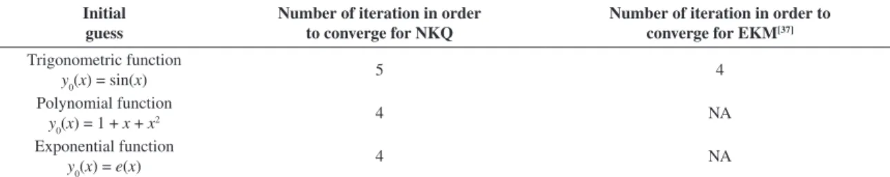
The plate is a square with 0.5 m length and 0.01 m thickness. A trigonometric function is chosen for initial guess (y0(x) = sin (πx/l)). It is shown in Figure 3 that it is converged after five iterations. Aghdam and Falahatgar37
used an Extended Kantorovich method EKM for analysing the thick composite plate. By choosing a trigonometric function as an initial guess, the model converges after 4 iterations.
In Table 1 the number of iterations, which are needed for convergence, for three different initial functions are shown. As it is mentioned earlier the initial guess does not have to satisfy the boundary conditions, so any initial function can be selected. Furthermore, as it is shown in Table 1 that the NKQ method is relatively quick and does not significantly depend on the initial value. The main advantage of this method, compared to EKM, is that it can be used for more where the secondary variables of the formulation are:
Nn≡ Nxxnx + Nxyny
Ns ≡ Nxynx + Nyyny
(36)
Mn≡ Mxxnx + Mxyny
Ms ≡ Mxynx + Myyny
(37)
0 0
0 0
n x xx xy x
y xy yy y
w w
V Q N N n
x y
w w
Q N N n
x y
∂ ∂
= + +
∂ ∂
∂ ∂
+ + +
∂ ∂
(38)
Equations 31-35 can be estimated by considering them as Urysohn form and an initial solution y0(x) and consequently the Y(0), A(0), F(0) and also repeating the
sequences for Equation 19.
Figure 3. Convergence of NKQ method.
Table 1. Number of iteration for convergence of NKQ and EKM.
Initial guess
Number of iteration in order to converge for NKQ
Number of iteration in order to converge for EKM[37]
Trigonometric function
y0(x) = sin(x) 5 4
Polynomial function
y0(x) = 1 + x + x2 4 NA
Exponential function y0(x) = e(x)
4 NA
Table 2. Relative error for CFFF boundary condition.
Number of iterations 1 2 3 4 5 6 7 8 9 10
Relative error (%) for u 29.4 8.3 3.4 1.9 1.1 0.6 0.3 0.1 0.0 0.0
Relative error (%) for v 34.5 9.2 5.1 2.1 1.2 0.8 0.3 0.1 0.0 0.0
Relative error (%) for w 53.4 11.3 5.4 2.1 1.2 0.8 0.4 0.2 0.0 0.0
Table 3. Relative error for SSSS boundary condition.
Number of iterations 1 2 3 4 5 6 7 8 9 10
Relative error (%) for u 25.4 9.1 3.9 1.9 1.2 0.7 0.4 0.1 0.0 0.0
Relative error (%) for v 47.2 11.0 5.6 2.5 1.5 1.0 0.5 0.2 0.1 0.0
Relative error (%) for w 76.6 21.2 7.0 2.9 1.5 0.9 0.5 0.2 0.1 0.1
E1 = 215Gpa E2 = E3 = 23.6Gpa, v12 = v13 = .17, v23 = .28 G12 = G13 = 5.4Gpa G23 = 2.1Gpa
The plate is a square and each length is 0.25 m, the thickness is 0.006 m and the lay ups are [0°, 90°, 0°]s . In Table 2 the relative error between the NKQ method and FEM for different numbers of iterations are shown for a plate clamped on one side (C) and free (F) on the other three
sides (CFFF). This example was then repeated for SSSS and CCCC boundary conditions and the results are shown in Tables 3, 4 respectively.
In Table 5, the dimensionless deflection at the centre of plate is compared between FEM, multi-term extended Kantorovich method (MTEKM) and NKQ method under different levels of load (patch out-of-plane load)16. As shown,
illustrate less than 3% error. The structure is a square plate with CFCC boundary conditions. The angle-ply laminated plate has four symmetric layers [45, –45].
In the next example a square laminated plate with a length of 0.5 m under uniform loading is considered. The plate is clamped at one side and the deformation at the other edge is measured. Because of the different lay-ups (anisotropic) and out-of-plane loading there is an induced twist at the free edge of the plate. The aim of this example is to find out if the NKQ model can estimate this induced twist.
The results are shown for an experiment, FEM and NKQ method in Figure 4. Carbon fibre is used for all laminated experimental tests and the size of plate is 500*500 (mm). The experimental test results which are shown in Figure 4 are the average results of six identical plates under the constant load.
5. Conclusion
The constitutive equations of the laminated composite plates are non-linear. The semi-analytical non-linear methods are an essential tool that provides perception to the physical non-linear behaviour of the composite plate structure, present fast and reliable solutions during the preliminary design phase and also provide a means of validations the numerical methods and enable the development of new computational models. In this paper a semi-analytical approach for the analysis of laminated plates with general boundary conditions and distribution of loads is proposed. The non-linear equations are solved by Newton-Kantorovich-Quadrature (NKQ) method. This method breaks down the laminate composite plate equations into a series of sequential equations and attempts to solve iterative linear integral equations. The convergence of the proposed method is compared with other semi-analytical methods (EKM and MTEKM). Various numerical examples with different boundary conditions and loadings are studied. Good agreement between the NKQ model, FEM and experimental results are shown to validate the model.
Table 5. Dimensionless W/h for CFCC square laminated plate under different loads.
Q MTEKM (W)[16] NKQ (W) ABAQUS %MTEKM Error[16] %NKQ Error
2488 .746 .741 .763 2.23 2.88
4975 1.092 1.090 1.115 2.05 2.24
7463 1.328 1.325 1.335 2.02 1.50
9950 1.512 1.559 1.541 1.81 1.16
12438 1.667 1.667 1.695 1.66 1.66
14925 1.800 1.802 1.827 1.54 1.36
17413 1.919 1.913 1.947 1.43 1.74
19900 2.027 2.025 2.053 1.33 1.36
Table 4. Relative error for CCCC boundary condition.
Number of iterations 1 2 3 4 5 6 7 8 9 10
Relative error (%) for u 92.2 30.4 14.1 8.3 5.3 3.2 1.8 1.0 0.4 0.1
Relative error (%) for v 63.8 19.2 9.2 5.1 3.7 1.9 0.9 0.4 0.1 0.0
Relative error (%) for w 77.1 24.5 11.1 6.6 4.9 2.2 1.3 0.7 0.3 0.1
Figure 4. Deformation at free edge of anisotropic laminated plate.
References
1. Khandan R, Noroozi S, Sewell P, Vinney J and Koohgilani M. Optimum Design of Fibre Orientation in Composite Laminate
Applied Mechanics. 1961; 28:402-408. http://dx.doi. org/10.1115/1.3641719
4. Stavsky Y. Bending and Stretching of Laminated Aeolotropic Plates. Journal of Engineering Mechanics ASCE. 1961; 87(6):31-56.
5. Dong SB, Pister KS and Taylor RL. On the Theory of Laminated Anisotropic Shells and Plates. Journal of Aeronautical Science. 1962; 29(8):969-975.
6. Yang PC, Norris CH and Stavsky Y. Elastic Wave Propagation in Heterogeneous Plates. International Journal of Solids and Structures. 1966; 2:665-684. http://dx.doi.org/10.1016/0020-7683(66)90045-X
7. Ambartsumyan SA. Theory of Anisotropic Plates. [translated from Russian by T. Cheron]. Stamford: Technomic; 1969.
8. W h i t n e y J M a n d L e i s s a AW. A n a l y s i s o f
Heterogeneous Anisotropic Plates. Journal of Applied
M e c h a n i c s . 1 9 6 9 ; 3 6 ( 2 ) : 2 6 1 - 2 6 6 . h t t p : / / d x . d o i . org/10.1115/1.3564618
9. Reddy JN. Mechanics of Laminated Composite Plates And Shells. 2nd ed. New York: CRC Press; 2004.
10. Reissner E. The effect of transverse shear deformation on the bending of elastic plates. Journal of Applied Mechanics. 1945; 12:69-77.
11. Mindlin RD. Influence of rotary inertia and shear on flexural motions of isotropic elastic plates. Journal of Applied Mechanics. 1951; 18:31-36.
12. Liew KM, Wang J, Tan MJ and Rajendran S. Nonlinear analysis of laminated composite plates using the mesh-free kp-Ritz method based on FSDT. Computer Methods in Applied Mechanics and Engineering. 2004; 193:4763-4779. http:// dx.doi.org/10.1016/j.cma.2004.03.013
13. Savithri S and Varadan TK. Large deflection analysis of laminated composite plates. International Journal of Non-Linear Mechanics. 1993; 28(1):1-12. http://dx.doi. org/10.1016/0020-7462(93)90002-3
14. Renganathan K, Nageswara Rao B and Manoj T. Moderately large deflection of laminated thin rectangular plates. ZAMM - Journal of Applied Mathematics and Mechanics/Zeitschrift für Angewandte Mathematik und Mechanik. 2002; 82(5):352-360. http://dx.doi.org/10.1002/1521-4001(200205)82:5<352::AID-ZAMM352>3.0.CO;2-H
15. Tanriöver H and Senocak E. Large deflection analysis of unsymmetrically laminated composite plates: analytical– numerical type approach. International Journal of Non-Linear Mechanics. 2004; 39:1385-1392. http://dx.doi.org/10.1016/j. ijnonlinmec.2004.01.001
16. Shufrin I, Rabinovitch O and Eisenberger M. A semi-analytical approach for the non-linear large deflection analysis of laminated rectangular plates under general out-of-plane loading. International Journal of Non-Linear Mechanics. 2008;43:328-340. http://dx.doi.org/10.1016/j. ijnonlinmec.2007.12.018
17. Akhras G, Cheung MS and Li W. Geometrically nonlinear
finite strip analysis of laminated composite plates. Composites
Part B. 1998; 29:489-495.
http://dx.doi.org/10.1016/S1359-8368(97)00038-3
18. Dawe DJ. Use of the finite strip method in predicting the behaviour of composite laminated structures. Composite
Structures. 2002; 57(1-4):11-36. http://dx.doi.org/10.1016/
S0263-8223(02)00059-4
19. Yang J and Zhang L. Nonlinear analysis of imperfect laminated thin plates under transverse and in-plane loads and resting on an elastic foundation by a semianalytical approach. Thin-Walled
Structures. 2000; 38:195-227. http://dx.doi.org/10.1016/
S0263-8231(00)00045-8
20. Rabinovitch O. Geometrically non-linear behavior of piezoelectric laminated plates. Smart Materials and
Structures. 2005; 14:785-798.
http://dx.doi.org/10.1088/0964-1726/14/4/038
21. Han SC, Tabiei A and Park WT. Geometrically nonlinear analysis of laminated composite thin shells using a modified first-order shear deformable element-based Lagrangian shell element. Composite Structures. 2008; 82:465-474. http:// dx.doi.org/10.1016/j.compstruct.2007.01.027
22. Reddy JN. Energy and Variational Methods in Applied Mechanics. John Wiley & Sons; 1984.
23. Kant T and Swaminathan K. Estimation of transverse/ interlaminar stresses in laminated composites: a selective review and survey of current developments. Composite
Structures. 2000; 49:65-75.
http://dx.doi.org/10.1016/S0263-8223(99)00126-9
24. Di Sciuva M and Icardi U. Analysis of thick multilayered anisotropic plates by a higher-order plate element.
American Institute of Aeronautics and Astronautics
Journal. 1995; 33(12):2435-2442.
25. Ramesh SS, Wang CM, Reddy JN and Ang KK. Computation of stress resultants in plate bending problems using higher-order triangular elements. Engineering Structures. 2008; 30:2687-706. http://dx.doi.org/10.1016/j.engstruct.2008.03.003 26. Carrera E and Demasi L. Classical and advanced multilayered
plate elements based upon PVD and RMVT. Part 1: derivation of finite element matrices. International Journal for Numerical
Methods in Engineering. 2002; 55:191-231. http://dx.doi.
org/10.1002/nme.492
27. Carrera E and Demasi L. Classical and advanced multilayered plate elements based upon PVD and RMVT. Part 2: numerical implementations. International Journal for Numerical Methods
in Engineering. 2002; 55:253-91. http://dx.doi.org/10.1002/
nme.493
28. Ramesh SS, Wang CM, Reddy JN and Ang KK. A higher-order plate element for accurate prediction of interlaminar stresses in laminated composite plates. Composite
Structures. 2009; 91:337-357 http://dx.doi.org/10.1016/j.
compstruct.2009.06.001
29. Cho M and Parmerter R. Finite element for composite plate bending on efficient higher order theory. American Institute
of Aeronautics and Astronautics Journal. 1994; 32:2241-8.
30. Oh J and Cho M. A finite element based on cubic zig-zag plate theory for the prediction of thermo-electric-mechanical behaviors. International Journal of Solids and
Structures. 2004; 41:1357-75. http://dx.doi.org/10.1016/j.
ijsolstr.2003.10.019
31. Kim KD, Liu GZ and Han SC. A resultant 8-node solid-shell element for geometrically nonlinear analysis. Computational
Mechanics. 2005; 35(5):315-31. http://dx.doi.org/10.1007/
s00466-004-0606-9
32. Kreja I and Schmidt R. Large rotations in first-order shear deformation FE analysis of laminated shells. International
Journal of Non-Linear Mechanics. 2006; 41(1):101-23. http://
dx.doi.org/10.1016/j.ijnonlinmec.2005.06.009
34. Liew KM, Zhao X and Ferreira AJM. A review of meshless methods for laminated and functionally graded plates and
shells. Composite Structures. 2011; 93:2031-2041. http://
dx.doi.org/10.1016/j.compstruct.2011.02.018
35. Saberi-Nadjafi J and Heidari M. Solving nonlinear integral equations in the Urysohn form by Newton-Kantorovich-quadrature method. Computers and Mathematics with
Applications. 2010; 60:2058-2065. http://dx.doi.org/10.1016/j.
camwa.2010.07.046
36. Kim HS, Cho M and Kim GI. Free-edge strength analysis in composite laminates by the extended Kantorovich method.
Composite Structures. 2000; 49:229-235. http://dx.doi.
org/10.1016/S0263-8223(99)00138-5
37. Aghdam MM and Falahatgar SR. Bending analysis of thick laminated plates using extended Kantorovich method.
Composite Structures. 2003; 62:279-283. http://dx.doi.
org/10.1016/j.compstruct.2003.09.026
38. Ungbhakorn V and Singhatanadgid P. Buckling analysis of symmetrically laminated composite plates by the extended Kantorovich method. Composite Structures. 2006; 73:120-128. http://dx.doi.org/10.1016/j.compstruct.2005.02.007
39. Yuan S and Jin Y. Computation of elastic buckling loads of rectangular thin plates using the extended Kantorovich method.
Composite Structures. 1998; 66(6):861-867. http://dx.doi.
org/10.1016/S0045-7949(97)00111-9
40. Shufrin I, Rabinovitch O and Eisenberger M. Buckling of symmetrically laminated rectangular plates with general boundary conditions; a semi analytical approach. Composite
Structures. 2008; 82:521-531. http://dx.doi.org/10.1016/j.
compstruct.2007.02.003
41. Soong TC. A procedure for applying the extended Kantorovich method to non-linear problems. Journal of
Applied Mechanics. 1972; 39(4):927-934. http://dx.doi.
org/10.1115/1.3422893
42. Daniel IM and Ishai O. Engineering Mechanics of Composite
Materials. 2nd ed. Oxford University Press; 2006.
43. Atkinson KE. A survey of numerical methods for solving nonlinear integral equations. Journal of Integral Equations and
Applications. 1995; 4:15-46. http://dx.doi.org/10.1216/
jiea/1181075664
44. Atkinson KE. The Numerical Solution of Integral Equations of
the Second Kind. Cambridge University Press; 1997. http://
dx.doi.org/10.1017/CBO9780511626340
45. Baker CTH and Miller GF. Treatment of Integral Equations by
Numerical Methods. London: Academic Press Inc.; 1982
46. Delves LM and Mohamed JL. Computational Methods for
Integral Equations. Cambridge University Press; 1985. http://
dx.doi.org/10.1017/CBO9780511569609
47. Jerri AJ. Introduction to Integral Equations with
Applications. 2nd ed. John Wiley and Sons; 1999
48. Kondo J. Integral Equations. Oxford: University Press, Kodansha Ltd; 1991
49. Kythe PK and Puri P. Computational Methods for Linear
Integral Equations. Boston: Birkhauser; 2002. http://dx.doi.
org/10.1007/978-1-4612-0101-4
50. Appell J, De Pascale E and Zabrejko PP. On the application of the Newton-Kantorovich method to nonlinear integral equations of Uryson type. Numerical Functional Analysis
and Optimization. 1991; 12(3-4):271-283. http://dx.doi.
org/10.1080/01630569108816428
51. Polyanin AD and Manzhirov AV. Handbook of Integral Equations. CRC Press; 2008. http://dx.doi.org/10.1201/9781420010558 52. Herakovich CT. Mechanics of fibrous composites. New York: