Article
Printed in Brazil - ©2013 Sociedade Brasileira de Química0103 - 5053 $6.00+0.00A
*e-mail: [email protected]
Quantum Second Virial Coefficient Calculation for the
4He Dimer on a Recent Potential
Éderson D’Martin Costa,a Nelson H. T. Lemes,a Márcio O. Alves,b
Rita C. O. Sebastiãob and João P. Braga*,b
aInstituto de Química, Universidade Federal de Alfenas,
Rua Gabriel Monteiro da Silva, 700, Centro, 37130-000 Alfenas-MG, Brazil.
bDepartamento de Química, Universidade Federal de Minas Gerais,
Av. Antônio Carlos, 6627, Pampulha, 31270-010 Belo Horizonte-MG, Brazil.
Este trabalho concentra-se no cálculo do segundo coeficiente virial quântico, a partir de um potencial desenvolvido recentemente. Este coeficiente foi determinado com 4-5 algarismos significativos na faixa de temperatura de 3 a 100 K. Nossos resultados estão dentro do erro experimental. Três contribuições para o valor total deste coeficiente são o espalhamento quântico (contribuição de estados no contínuo), o estado ligado (contribuição de estados discretos) e o gás ideal quântico; discutimos estas contribuições separadamente. A contribuição mais importante é do espalhamento quântico, enquanto que as contribuições menores são dos estados discretos. Uma análise da sensibilidade foi realizada em função da temperatura para um parâmetro na região de curto alcance do potencial e para três parâmetros na região de longo alcance do potencial. Para ambas as temperaturas consideradas, 10 e 100 K, o coeficiente de dispersão C6 foi o mais significativo, e o termo dispersão C10 foi o menos significativo para o resultado total. Em geral, a
precisão exigida para descrever os potenciais diminui com o aumento da temperatura. A precisão total e a relação dos parâmetros com os erros experimentais são discutidas.
This paper focuses on the calculation of the quantum second virial coefficient, under a recently developed potential. This coefficient was determined to within 4-5 significant figures in the temperature range from 3 to 100 K. Our results are within experimental error. The three contributions to the overall value of the coefficient are the quantum scattering (continuum state contribution), the bound state (discrete state contribution) and the quantum ideal gas; we discuss these contributions separately. The most significant contribution is from the scattering states, whereas the smaller contributions are from the discrete states. A sensitivity analysis was performed as a function of temperature for one parameter in the short-range region of the potential and for three parameters in the long-range regions of the potential. For both temperatures considered, 10 and 100 K, the C6 dispersion coefficient was the most significant, and the C10 dispersion term was the least significant to the overall result. In general, the precision required to describe the potential decays as the temperature increases. The overall accuracy and the relationship of the parameters to the experimental errors are discussed.
Keywords: quantum virial, helium-helium, scattering phase shift.
Introduction
A quantum second virial coefficient calculation provides important information that is necessary for analyzing model potentials, for this calculation involves low temperature data.1 These potential energy function
can be obtained by a direct procedure, such as fitting parameters to experimental data, or, conversely, by
an inverse problem treatment, in which experimental properties are treated first.2-5 The potential refinement is
very important in chemistry and is performed whenever new reliable data become available. Accurate values of helium properties, such as the low-temperature experimental virial coefficient, can be determined6-8
and experimental 4He
2 dimers can be identified.9-15
Several He-He intermolecular potentials are discussed in the literature.16-20 The most recent potential has not
been tested against thermodynamic and transport property data,21 such as the quantum second virial coefficients. In the
present work, a study of this recent potential was conducted using second virial coefficient data at low temperature.The quantum virial coefficient can be determined by evaluating the quantum ideal gas term, the scattering phase shift dependence on angular momentum22-29 and the bound states
by Levinson’s theorem.25-26
This low-temperature second virial coefficient calculation is an important step to test the quality of the potential under consideration. Together with this quantum calculation, a sensitivity analysis on the dispersion coefficients is also performed. This test is very important, especially in low energy conditions when the potential parameters are more sensitive. The results obtained in the present work will be compared to experimental data for the helium-helium system.22-24
Experimental
The partial wave method
A numerical solution to the Schrödinger equation is the first step to providing information about the quantum virial coefficient. In the scattering process, the Schrödinger equation can be written as
(1)
where k2 = 2µE/ħ2, l is the angular momentum, µ is the
reduced mass and E is the energy of the relative motion.
After the collision process, the scattered wave function is
(2)
The phase shift, δl, carries all of the necessary
information to describe the scattering, as it represents a phase that is accumulated along the scattering process with respect to a free particle. If no potential were present, the phase shift would be zero. The phase shift was calculated by the renormalized Numerov method, which is a very robust numerical procedure for solving equation 1.30 Riccati-Bessel functions were used to match
Schrödinger equation solutions at a maximum scattering coordinate.31 At this point, wavefunction continuity are
imposed and the scattering matrix (or phase shift) can be established.32
Quantum virial coefficient
The equation of state for the helium system can be represented by p/kBT = r + B(T)2, in which r is the density
and B(T) is the second virial coefficient. The classical
second virial coefficient is not appropriate to describe the helium equation of state at temperatures lower than 100 K.22 Instead, the exact quantum second virial coefficient
expression relating the phase shift and the energy of bound state is used for an accurate system description.6,23,24 The
molar virial expansion is represented in the form
(3)
in which e is the He2 binding energy for zero angular
momentum, kB is Boltzmann’s constant and
(4)
with = 2.556 Å. The dimensionless variables q and q0 were
conveniently introduced in formulating the problem and are related to the collision energy and temperature, respectively. For further comparison, if q = 1 for the system under
consideration, the collision energy will be E = 1.60 × 10⁻⁴ eV.
Moreover, q0 = 1 will correspond to T = 1.85 K. Other
transformations can be obtained with this reference. As the energy increases, the phase shift will gradually approach zero, and the integral term in equation 3 will converge.
For the 4He dimer, the ideal part of the second virial
coefficient, Bideal, considers the Bose statistics, and no
intermolecular forces are considered.33 This term is
important at low temperature and approaches zero at higher temperature. The inclusion of the discrete energy levels, with only one rovibrational state for He2 in the partition
function, gives rise to the second term in equation 3,
Bbound. A contribution from the scattering states comes
from the third term, Bphase, in which the phase shift has
to be considered. This term is the most important one in establishing the second virial coefficient for the helium system.22
Potential energy function
For the description of the system, an accurate potential developed by Varandas21 was employed. This potential is
(5)
and
(6)
are used to define the potential. The function, Xn(R), is
(7)
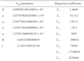
The value in atomic units of the damping function coefficients are: = 10.9424025 , a0 = 16.36606, a1 = 0.70172, b0 = 17.19338 and b1 = 0.09574. The other
necessary parameters to determine the potential are given in Table 1.
Data in the literature16-20 show that the He dimer
potential well at 10.9 K and a nuclear equilibrium distance of 2.97 Å only support a single bound rovibrational state with a binding energy of approximately –1.176 mK,34
which is the weakest bound state ever discovered. Due to this extremely weak interaction, the wave function must be delocalized over a large intermolecular distance. The mean intermolecular distance for He at the ground state is approximately 50 Å.9-15
The minimum energy value (D = 11.0 K) and the
equilibrium distance (Re = 2.965 Å) predicted by the
potential used here are in agreement with previous results in the literature.16-21 This proposed potential energy curve
is investigated, by comparing the calculated exact quantum second virial coefficient with the experimental results at low temperatures.
The quantum scattering calculation
Calculation of the quantum second virial coefficient requires a solution to Schrödinger’s equation and, after appropriate boundary conditions, the quantum phase shift calculation. The renormalized Numerov algorithm that propagates the ratio of wave functions was used to calculate the scattering matrix from which the phase shift was found.30 Propagating the ratio of the wave function at
two consecutive points, such as is the essential idea behind this renormalized method; here, h is the
integration step size. This procedure will provide a very stable propagator, even into the classically forbidden regions. A critical analysis of this method appears in the literature.35
Levinson’s theorem relates the zero energy phase shift to the number of bound states supported by the potential using
dl(q→0) = nlπ (8)
Here, nl is the number of bound states for the
given angular momentum.35 The 4He
2 molecule was
experimentally detected by several groups.9-15 For l ≥ 1
the helium molecule was not detected, a fact that was also confirmed numerically in this study.
For large angular momentum states, the centrifugal term will dominate the collision process, and the scattering process will occur with negligible changes in potential energy. At this point, phase shift will decrease to zero. Therefore, the quantity G(q), which is necessary to calculate the second
virial coefficient, will converge for a maximum angular momentum, lmax.6,23 By angular momentum conservation, one
can estimate this maximum at lmax≈kRmax, in which Rmax is
the potential range. The quantity lmax is the maximum angular
momentum required to achieve cross section convergence. The quantity is shown in Figure 1, using the Varandas potential. The maximum angular moment in the range of 20 < lmax < 80 gives a convergence
of at least 4(lower temperatures)-5(higher temperatures) significant figures for energies in the range 0 < q < 80.
The G(q) curve presents a primary peak near q = 0, which
is predicted by Levinson’s theorem. As observed for temperatures under 30 K, the integration process must be performed until q = 14, which is the convergence point for
the energy. The phase shifts were calculated at intervals of ∆q = 0.005. Numerical integration was performed
using Simpson’s method together with a cubic spline interpolator.36,37 Integrated results were confirmed to be
within 4-5 significant figures.
Table 1. Parameters for the helium potential in atomic units21
VHFparameters Dispersion coefficients
D 2.909582149142803 × 10⁻⁵ C
6 1.4646
a1 –2.677678262034801 × 10⁻¹ C8 14.112
a2 2.345720241868299 × 10⁻² C10 178.13
a3 1.459174818996908 × 10⁻² C11 –76.7
a4 1.237617600368155 × 10⁻⁵ C12 3093
Re 5.60323206384019 C13 –3806.0
g 2.17613250152118 C14 72016
C15 –171000.0
Results and Discussions
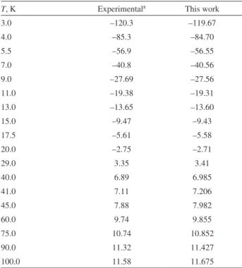
The present calculation of the quantum second virial coefficient was performed with 4-5 significant figures, and the results are shown in Table 2. A comparison is made with experimental and theoretical calculation. The second virial coefficient error calculated in the present work is within 0.1 cm3 mol–1 for temperatures above 10 K,
but this result increases to 0.63 cm3 mol–1 for T = 3 K.
Guided by the experimental error of 0.6 cm3 mol–1 for
lower temperatures, one may conclude that the potential used in the present calculation is appropriate in this temperature range.8,38
Term contribution
We discuss the individual contributions to the second virial coefficient expansion in equation (3). The first term is a Bose-Einstein ideal gas contribution, the second term is the bound state contribution, and the third term is related to atomic interaction as determined by the phase shift information.
The quantum ideal gas term,33
(9)
is significant at low temperature and decreases in importance as the temperature is increased. For example, this term contributes approximately 11% at 3 K and 0.7% at 100 K. Due to the Bose-Einstein statistics, this contribution is always negative for the second virial coefficient. For room temperature, this term can be neglected.
The existence of a 4He diatomic molecule for the
potential under consideration makes it necessary to consider the bound state term,
(10)
This contribution to virial expansion represents 0.07% at 3 K and decreases at large temperatures to 10–4% at
100 K; these values are much smaller than the ideal quantum gas correction. In fact, error in the bound state energy will not have a considerable effect on the second virial coefficient data.
However, the phase shift contribution to virial calculation,
(11)
is significant; therefore, quantum virial coefficient data at low temperatures are a good test of novel potential functions. For example, Bphase at 3 K represents 88.6% of
the total contribution to the coefficient. In Table 3, we show the individual contributions of these three terms from 3 K to 100 K.
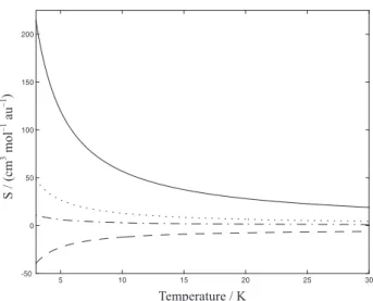
Sensitivity analysis
An important issue involves the question of how the potential energy function has to be to reproduce a desired property. The answer is provided by the sensitivity analysis.39 This question was analyzed, and the results Figure 1. A plot of the function g(q) = G(q)qe–q2/q
02 at T = 30 K.
Table 2. Second virial coefficients for 4He in units of cm3 mol–1
T, K Experimental8 This work
3.0 –120.3 –119.67
4.0 –85.3 –84.70
5.5 –56.9 –56.55
7.0 –40.8 –40.56
9.0 –27.69 –27.56
11.0 –19.38 –19.31
13.0 –13.65 –13.60
15.0 –9.47 –9.43
17.5 –5.61 –5.58
20.0 –2.75 –2.71
29.0 3.35 3.41
40.0 6.89 6.985
41.0 7.11 7.206
45.0 7.88 7.982
60.0 9.74 9.855
75.0 10.74 10.852
90.0 11.32 11.427
are shown in Table 4. Accordingly, the uncertainties established are greater than those established with the Varandas potential.21
The sensitivity of the second virial coefficient is greater for the C6 dispersion term and smaller for the C8
and C10 terms; these results are presented in Figure 2. The
short-range g Born-Mayer type parameter importance, shown in the figure, is as relevant as the C8 term. The
temperature dependence of the potential parameters is the important information that is obtained from Figure 2. It is clear that all terms become less important as the temperature is increased.
The second virial coefficient experimental error will be assumed to be ± 0.01 cm3 mol–1,8 which is below the
average experimental error. One might then ask what
will the allowed error in the potential parameter be, at a given temperature, to give this experimental error. As stated in the potential model used here,21 the errors in
the dispersion coefficient C6, C8 and C10 are 10–12, 10–8
and 10–6, respectively. This result is not compatible with
the sensitivity of the dispersion coefficient, as presented in Table 4. The variation in these parameters, even for 100 K, is well below the data used in the construction of the potential model.21 For lower temperatures, the variation
in these parameters is more restricted but still below the assumed experimental error.
A family of potential energy curves is an acceptable method used to reproduce the second quantum virial coefficient. For example, the potential used in the present work is similar to other potentials in the literature,16 and the
calculated quantum second virial coefficient will provide data within experimental error if these potentials are used; we emphasize this point in Table 2. Experimental error provides a rule to be followed in modeling potential energy function. Therefore, if accurate information is used, such as the quantum second virial data, important restriction on the potential model is imposed.
Conclusions
Quantum second virial coefficient for the 4He
2 system
were calculated in the present work for a novel potential over the temperature range from 3 to 100 K. Calculations in this temperature range showed classical or semi-classical behavior that were not sufficient to adequately describe the second virial data. Our results are in agreement with experimental errors. For example, the difference between our theoretical results and the experimental data are 0.63 cm3 mol–1 for T = 3 K and 0.095 cm3 mol–1 for T = 100 K. Table 3. Calculated quantum second virial coefficient contribution terms
in cm3 mol–1
T B Bphase Bideal Bbound
3.0 –119.67 –105.97 –13.614 –8.5402 × 10⁻²
4.0 –84.698 –75.814 –8.8424 –4.1601 × 10⁻²
5.5 –56.552 –51.049 –5.4842 –1.8764 × 10⁻²
7.0 –40.563 –36.733 –3.8196 –1.0268 × 10⁻²
9.0 –27.564 –24.939 –2.6200 –5.4778 × 10⁻³
11.0 –19.307 –17.365 –1.9390 –3.3169 × 10⁻³
13.0 –13.604 –12.093 –1.5092 –2.1845 × 10⁻³
15.0 –9.4351 –8.2159 –1.2177 –1.5275 × 10⁻³
17.5 –5.5823 –4.6150 –0.96628 –1.0390 × 10⁻³
20.0 –2.7118 –1.9202 –0.79089 –7.4409 × 10⁻⁴
29.0 3.4108 3.8640 –0.45296 –2.9390 × 10⁻⁴
40.0 6.9847 7.2644 –0.27962 –1.3154 × 10⁻⁴
41.0 7.2062 7.4758 –0.26945 –1.2366 × 10⁻⁴
45.0 7.9821 8.2165 –0.23434 –9.7986 × 10⁻⁵
60.0 9.8550 10.007 –0.15221 –4.7732 × 10⁻⁵
75.0 10.852 10.960 –0.10891 –2.7324 × 10⁻⁵
90.0 11.427 11.509 –0.082851 –1.7321 × 10⁻⁵
100.0 11.675 11.746 –0.070739 –1.3299 × 10⁻⁵
Table 4. Acceptable parameter deviation for ∆B = 0.01 in cm3 mol–1 and
atomic units
Parameter Sensitivity Deviation Error21
T = 10 K C6 50 2 × 10⁻⁴ 10–12
C8 10 10–3 10–8
C10 1 10–2 10–6
g 10 10–3 –
T = 100 K C6 10 10–3 10–12
C8 1 10–2 10–8
C10 1 10–2 10–6
g 5 2 × 10⁻³ –
Figure 2. Parametric sensitivity analysis for C6 (–), C8 (…), C10 (--) and
Contributions from the bound state term, the Bose-Einstein interaction and the phase shift were discussed. The first two terms showed a small influence on this coefficient. For example, at 3 K, the bound state contribution is 0.07% and the Bose-Einstein is 11%, while at the same temperature, the phase shift term contributes 89% to the total second virial coefficient.
Under the inverse problem theory framework, a potential parameter sensitivity analysis was also studied. The calculated uncertainties in the parameter were, in fact, greater than the precision used to construct the potential used in the present calculation. For example, to be within experimental error, the dispersion coefficient C6 can have
uncertainty as small as 10–4 au, which is well above the
theoretical calculation of 10–14 au.
Theoretical calculations with the potential function proposed by Varandas and used in the present work are within experimental error. In fact, it was difficult to select the best potential that describes helium-helium interaction at low temperatures. Sensitivity analysis has shown that the precision in the potential parameters is beyond that which is required to reproduce the experimental quantum second virial coefficient; therefore, a set of potentials is acceptable.
Acknowledgments
We would like to thank CNPq, CAPES and FAPEMIG for financial support.
References
1. Pethick, C. J.; Smith, H.; Bose-Einstein Condensation in Dilute Gases; Cambridge University Press: Cambridge, 2002. 2. Lemes, N. H. T; Braga, J. P; Belchior, J. C.; Chem. Phys. Lett.
1998, 296, 233.
3. Braga, J. P; de Almeida, M. B.; Braga, A. P.; Belchior, J. C.;
Chem. Phys.2000, 260, 347.
4. Sebastião, R. C. O.; Lemes, N. H. T; Virtuoso, L. S.; Braga, J. P.; Chem. Phys. Lett.2003, 378, 406.
5. Lemes, N. H. T; Sebastião, R. C. O.; Braga, J. P.; Inverse Probl. Sci. En.2006, 14, 581.
6. Colclough, A. R.; Metrologia1979, 15, 183.
7. Kessler, W. D.; Osborne, D. V.; J. Phys. C: Solid St. Phys.1980,
13, 2097.
8. Steur, P. P. M.; Duriex, M.; McConville, G. T.; Metrologia1987,
24, 69.
9. Luo, F.; McBane, G. C.; Kim, G.; Giese, C. F.; Gentry, W. R.;
J. Chem. Phys.1993, 98, 3564.
10. Meyer, E. S.; Mester, J. C.; Silveira, I. F.; J. Chem. Phys.1994,
100, 4021.
11. Luo, F.; McBane, G. C.; Kim, G.; Giese, C. F.; Gentry, W. R.;
J. Chem. Phys.1994, 100, 4023.
12. Schöllkopf, W.; Toennies, J. P.; Science1994, 266, 1345. 13. Luo, F.; Giese, C. F.; Gentry, W. R.; J. Chem. Phys.1996, 104,
1151.
14. Schöllkopf, W.; Toennies, J. P.; J. Chem. Phys.1996, 104, 1155.
15. Focsa, C.; Bernath, P. F.; Colin, R.; J. Mol. Spectrosc.1998,
191, 209.
16. Przybytek, M. and Cencek, W.; Komasa, J.; Szalewicz, K.; Phys. Rev. Lett.2010, 104, 183003.
17. Hurly, J. J.; Mehl, J. B.; J. Res. Natl. Stand. Technol.2007, 112, 75.
18. Jeziorska, M.; Cencek, W.; Patkowski, K.; Jeziorski, B.; Szalewicz, K.; J. Chem. Phys.2007, 127, 124303.
19. Janzen, A. R.; Aziz, R. A.; J. Chem. Phys.1997, 107, 914. 20. Janzen, A. R.; Aziz, R. A.; J. Chem. Phys.1995, 103, 9626.
21. Varandas, A. J. C.; J. Phys. Chem., A 2010, 114, 8505. 22. Boyd, M. E.; Larsen, S. Y.; Kilpatrick, J. E.; J. Chem. Phys.
1969, 50, 4034.
23. Kilpatrick, J.; Keller, W.; Hammel, E.; Metropolis, N.; Phys. Rev.1954, 94, 1103.
24. Kihara, T.; Rev. Mod. Phys.1955, 27, 412.
25. Bernstein, B. R. In Atom-Molecule Collision Theory, A Guide For The Experimentalist; Bernstein, B. R., eds.; Plenum Press:
New York, 1979.
26. Murrell, J. N.; Bosanac, S. D. Introduction to the theory of atomic and molecular collisions; John Wiley & Sons: New York, 1989.
27. Siska, P. E.; Parson, J. M.; Schafer, T. P.; Lee, Y. T.; J. Chem. Phys.1971, 55, 5762.
28. Farrar, J. M.; Lee, Y. T.; J. Chem. Phys.1972, 56, 5801. 29. Burgmans, A. L. J.; Farrar, J. M.; Lee, Y. T.; J. Chem. Phys.
1976, 64, 1345.
30. Johnson, B. R.; J. Chem. Phys.1977, 67, 4086.
31. Abramowitz, M.; Stegun, I. A.; Handbook of Mathematical Functions Dover: New York, 1965.
32. Braga, J. P.; J. Comp. Chem.1989, 10, 413.
33. Huang, K.; Statistical Mechanics; John Wiley & Sons: New
York, 1987.
34. Grisenti, R. E.; Schollkopf, W.; Toennies, J. P.; Phys. Rev. Lett.
2000, 85, 2284.
35. Braga, J. P.; Murrell, J. N.; Mol. Phys.1984, 53, 295.
36. Forsythe, G. E.; Malcolm, M. A.; Moler, C. B.; Computer Methods for Mathematical Computations; Prentice-Hall: New
York, 1977.
37. McCongille, G. T.; Hurly, J. J.; Metrologia1991, 28, 375.
38. Berry, K. H.; Metrologia1979, 15, 89.
39. Ho, T.; Rabitz, H.; J. Chem. Phys.1988, 89, 5614.
Submitted: August 7, 2012