Time correlation function in systems with two coexisting biological species
E. Arashiro, A. L. Rodrigues, M. J. de Oliveira, and T. Tomé
*
Instituto de Física, Universidade de São Paulo, Caixa Postal 66318, 05315-970 São Paulo, São Paulo, Brazil 共Received 24 March 2008; revised manuscript received 19 April 2008; published 12 June 2008兲 We study a stochastic lattice model describing the dynamics of coexistence of two interacting biological species. The model comprehends the local processes of birth, death, and diffusion of individuals of each species and is grounded on interaction of the predator-prey type. The species coexistence can be of two types: With self-sustained coupled time oscillations of population densities and without oscillations. We perform numerical simulations of the model on a square lattice and analyze the temporal behavior of each species by computing the time correlation functions as well as the spectral densities. This analysis provides an appropriate characterization of the different types of coexistence. It is also used to examine linked population cycles in nature and in experiment.
DOI:10.1103/PhysRevE.77.061909 PACS number共s兲: 87.23.Cc, 87.10.Hk, 05.70.Ln
I. INTRODUCTION
The Lotka-Volterra model is the first one关1,2兴describing how the interaction between two biological species leads to time oscillations. This model consists of a set of two coupled ordinary differential equations for the density of prey and predator and is set up in analogy with the laws of mass action 关3–6兴. However, the Lotka-Volterra description does not take in an explicit way the spatial structure of the envi-ronment where the species coexist. One manner of taking into account the spatial structure is to consider lattice models in which the species individuals reside on the sites of the lattice and interact with its neighbors by stochastic local tran-sition rules 关7–13,15–27,29–31兴. These models are usually continuous time Markovian processes defined by discrete stochastic variables residing on the sites of the lattice, also called interacting particle system关32,33兴.
The stochastic transition rules embodied in the lattice model imply stochastic fluctuations in the number of a given species as a function of time. The stochasticity, which is ubiquitous in nature and is observed in real data, is also an essential ingredient of the stochastic lattice models, object of our analysis, but is absent in the Lotka-Volterra model. The stochastic lattice models, moreover, give a correct descrip-tion of the local time oscilladescrip-tions in the sense that the ampli-tude of the oscillations do not depend on the initial condi-tions. The oscillations coming from the stochastic lattice models are autonomous, or self-sustained, and depend only on the external parameter. The stochastic lattice model as well as some other approaches关34–38兴, incorporates the dis-creteness of the species individuals and local stochastic in-teractions which are important ingredients to describe cyclic fluctuation in population dynamics.
In the present work we study the coexistence and the emergence of stable local self-sustained oscillations in a sto-chastic lattice model that describes the interaction between two species, in particular, predator and prey species. Here we study a modified version of the model introduced by Satu-lovsky and Tomé 关8兴by including diffusion of species
indi-viduals. It has been pointed out that diffusion provides a more realistic description since the species individuals move themselves in their habitat 关27,39–45兴. We focus on the analysis of the time series by determining the time autocor-relation function of each species as well as the time cross-correlation function. As applications of this type of analysis we examine two examples of real data coming from coexist-ing biological species found in nature and in experiments.
II. MODEL
We depart from the stochastic lattice model for a predator-prey system关8兴. One considers a regular square lattice rep-resenting the habitat where the two interacting species coex-ist. Each site can be either empty or occupied by one individual of different species. The state of a site is described by a variableithat takes the values 0, 1, or 2, according to
whether the site is empty, occupied by a prey individual or by a predator, respectively. That is,
i=
冦
0, empty, 1, prey, 2, predator.
冧
共1兲
A microscopic state of the system is denoted by the stochas-tic vector=共1, . . . ,i, . . . ,N兲, where N is the total
num-ber of sites. The probabilityP共,t兲of configurationat time t evolves in time according to the master equation
d
dtP共,t兲=
兺
⬘
兵W共,
⬘
兲P共⬘
,t兲−W共⬘
,兲P共,t兲其, 共2兲where the summation is over all the microscopic configura-tions
⬘
共⫽兲of the system, andW共,⬘
兲is the rate of tran-sition共conditional probability per unit time兲from state⬘
to state .The transitions between the three states obey the cyclic order shown in Fig.1. The three processes are described as follows: Prey individuals are born in empty sites; prey indi-vidual dies and is instantaneously replaced by a new born predator; finally a predator can die leaving an empty site. The two first processes are catalytic whereas the third is spontaneous.
The predator-prey lattice model has three parameters: a, the probability of birth of prey,b, the probability of birth of predator and death of prey, andc, the probability of predator death. The occupancy of a site by prey or by a predator is conditioned, respectively, to the existence of prey or predator in the neighborhood of the site. The third reaction, where predator dies occurs with probabilityc, independently of the states of the neighboring sites. By rescaling time it is pos-sible to assume thata+b+c= 1, with 0ⱕa,b,cⱕ1. We use an auxiliary parameter p and write a=共1 −c兲/2 −p and b =共1 −c兲/2 +p.
More specifically, the transition probabilities are de-scribed in what follows:
共a兲If a siteiis empty共i= 0兲and there is at least one prey
individual in its first neighborhood, there is a favorable con-dition for the birth of a new prey. The probability of site i being occupied in the next time step by a prey is proportional to the parametera and to the number of prey individuals in the first neighborhood of the empty site. The transition prob-ability per site associated to this process is given by
wi共0→1兲=␦共i,0兲
a
4
兺
k␦共k,1兲, 共3兲
where the summation is over the four nearest neighbors of sitei in a regular square lattice. The notation␦共x,y兲 stands for the Kronecker␦ function.
共b兲If a site is occupied by a prey共i= 1兲and there is at
least one predator in its first neighborhood, then the site has a probability of being occupied by a new predator in the next time step. In this process the prey dies instantaneously. The transition probability is proportional to the parameter b and to the number of predators in the first neighborhood of the site. The transition probability for this process is
wi共1→2兲=␦共i,1兲
b 4
兺
k␦共k,2兲. 共4兲
共c兲If sitei is occupied by a predator共i= 2兲it dies with
probability c. The corresponding transition probability is given by
wi共2→0兲=c␦共i,2兲, 共5兲
These stochastic local rules define the dynamics of the stochastic lattice model for a predator-prey system without diffusion.
Here we consider a reaction-diffusion process by adding to the above transitions, related to the reactive processes, a diffusion process to mimic the explicit movement of prey. That is, with probability D a diffusion is attempted; with probability 1 −Done performs the transitions共a兲,共b兲, and共c兲 above. The diffusion is realized as follows. One site is cho-sen at random. Suppose it is occupied by one prey indi-vidual, there are n empty nearest-neighbor sites. Then the individual jumps to one of thenempty sites with equal prob-ability. In analogous way, if the chosen site is empty and there arennearest-neighbor prey individuals, one of them is chosen at random and jumps to the empty site. Otherwise, that is, if the chosen site is occupied by a predator state of sites remains unchanged.
III. TIME CORRELATION
To characterize the time behavior of the density of the two species, we measure the time autocorrelation function for each species and the time cross-correlation function between the two species. Let us denote by x共t兲 and y共t兲 the times series for the prey and predator, respectively, and let¯xand¯y be their respective average in time. We define the prey and predator time autocorrelation functions as
cx共t兲=
冕
关x共t⬘
+t兲−¯x兴关x共t⬘
兲−¯x兴dt⬘
共6兲and
cy共t兲=
冕
关y共t⬘
+t兲−¯y兴关y共t⬘
兲−¯y兴dt⬘
. 共7兲The time cross-correlation function between prey and preda-tor is given by
cxy共t兲=
冕
关x共t⬘
+t兲−¯x兴关y共t⬘
兲−¯y兴dt⬘
. 共8兲Instead of these correlations we use in actual calculations the normalized correlations, defined by
2
b
c
0
a
FIG. 1. Transitions of the predator-prey model. The three states are prey共1兲, predator共2兲, and empty共0兲. The allowed transitions obey the cyclic order shown.
rx共t兲=
cx共t兲
cx共0兲
, 共9兲
ry共t兲=
cy共t兲
cy共0兲
, 共10兲
rxy共t兲= cxy共t兲
cxy共0兲. 共11兲 For each of the two autocorrelation functions, we have determined the Fourier transform, given by
Sx共兲=
冕
rx共t兲eitdt, 共12兲Sy共兲=
冕
ry共t兲eitdt. 共13兲According to the Wiener-Kinchin theorem, Sx共兲 andSy共兲
may be identified with the power spectral density relative to prey and predator time series, respectively.
Let us assume that the correlation function is described, at least qualitatively, by the function
r共t兲=e−␥兩t兩f共t兲, 共14兲 where␥is a parameter describing the time decay and f共t兲is a periodic even function of time with a certain period. If we expand f共t兲in Fourier series we obtain
r共t兲=e−␥兩t兩
兺
n
Ancos共n0t兲, 共15兲
whereAn are the amplitudes and0is the main frequency.
The Fourier transform of the correlationr共t兲is then
S共兲=
兺
n
An
冉
␥ ␥2+共n0+兲2+ ␥
␥2+共n0−兲2
冊
,
共16兲
which has local maxima at =n0. For large values of ,
that is,Ⰷ␥, and assuming thatAndecreases rapidly withn,
we have FIG. 3. 共Color online兲 共a兲 Density of prey x and density of
predator y versus c for p= 0.3 and D= 0.9. 共b兲 The quantity 共1 −x兲1/ versus c, where = 0.58. The critical point occurs at c
c
= 0.320共5兲.
0 0.05 0.1 0.15 0.2 0.25 0.3
c
0 0.2 0.4 0.6 0.8
r
(a)
0.1 0.15 0.2 0.25 0.3
c
0 0.2 0.4 0.6 0.8
r
2(b)
FIG. 4. 共a兲Value of the cross-correlationrat the first maximum as a function of the parameterc, forp= 0.3 andD= 0.9.共b兲Plot of r2 as functions of c. The linear regression gives the value cⴱ
S共兲 ⬃ ␥
␣, ␣= 2, 共17兲
so that the log-log plot ofSversushas a slope␣= 2 char-acterizing the exponential decay of the correlation function. In the absence of oscillation we may describe the time autocorrelation function qualitatively by the following func-tion:
r共t兲=A0e−␥兩t兩, 共18兲
which may be understood as the expression共15兲in which all coefficients An vanish except the coefficient A0. Its Fourier
transform is given by the Lorentzian
S共兲= 2A0␥
␥2+2, 共19兲
and is a monotonic decreasing function of frequency. For large values of , that is, Ⰷ␥, the Fourier transform be-haves according to Eq.共17兲.
IV. NUMERICAL SIMULATION
The simulations of the stochastic lattice model were per-formed in a square lattice ofN= 160⫻160 sites starting from a random configuration of prey and predator in which each site has a probability 1/3 of being occupied by a predator and 1/3 of being occupied by a prey individual. The total number of Monte Carlo steps ranged from 105 to 106. At each time
step the configuration of the lattice was updated according to the stochastic rules presented in Sec. II. To explore the sev-eral possible states of the model we may use a phase diagram in the variablesp andcfor a given fixed value of the diffu-sion parameter D. Since we are concerned with the charac-terization of the time series, it suffices to consider a repre-sentative section of the phase diagram, which we choose to be p= 0.3 andD= 0.9. The choice ofDis discussed in what follows.
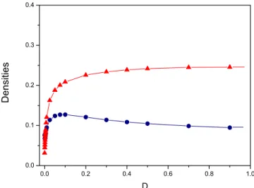
The explicit diffusion enhances the species coexistence and the oscillatory behavior. The introduction of the diffu-sion process promotes the increase of the average species densities as can be seen in Fig.2. Even a small value ofD suffices to entail this behavior as shown by the rapid increase FIG. 5. 共Color online兲 共a兲 Densities of prey共lower curve兲and predator共upper curve兲 as a function of time forp= 0.3,c= 0.03, andD = 0.9.共b兲Cross-correlation function between prey and predator.共c兲Time autocorrelation function for prey.共d兲Power spectral density for prey. The largest peak occurs at= 0.0057 which gives a periodT= 1.10⫻103. The second and the third peaks occur at= 0.0112 and
in the average species densities up to D⬵0.05. Above this value the average densities become almost constant indicat-ing that the behavior of the system is similar for values of D⬎0.05. It is therefore enough to study the properties of the system for just one point within this interval, which we choose here to beD= 0.9.
The present model predicts a state in which the lattice is full of prey, called prey absorbing state, in which the system cannot escape, remaining there forever. This absorbing state occurs if the parameterc, that regulates the death of predator, is sufficiently high. As one increases the external parameterc the system then shows a continuous phase transition from a state where the species coexist to a prey absorbing state. For D= 0.9 andp= 0.3, this occurs at a critical valueccas shown in Fig. 3, where the averagesx and y, density of prey and predator, respectively, are plotted as a function ofc. The prey absorbing state is characterized by x= 1 and y= 0. In this figure we have also plotted共1 −x兲1/as a function ofc. Since
we expect that this critical behavior belongs to the universal-ity class of direct percolation关25,29兴we used= 0.58. The straight line fitted to the data points corroborates this expec-tation and gives the valuecc= 0.320共5兲.
In the interval betweenc= 0 andc=ccthe system exhibits
the most interesting states, which are the active states where
prey and predator coexist. We distinguish two types of coex-istence: One with time oscillatory behavior, for small values of c, and the other without oscillations, which we call ordi-nary coexistence, for values of c near cc. Our numerical
study predicts the change from one behavior to another at c=cⴱ⬇0.28 for p= 0.3 andD= 0.9, as can be inferred from
Fig.4, and to be explained shortly.
In Figs.5–8we show the densities of prey and predator as functions of time for p= 0.3, D= 0.9 and for the following values of c: 0.03, 0.15, 0.25, and 0.29, respectively. We present also the time autocorrelation function for prey, the cross-correlation between prey and predator, and the Fourier transform of the autocorrelation of prey. For the first three values ofcthe system shows clear oscillations characterized by oscillating correlation functions whose amplitudes decay exponentially.
The plots in Figs.5–7, indicate that the correlation and the power spectral density are in qualitative agreement with Eqs. 共15兲 and共16兲. Moreover, the slope of the tail is equal to ␣ = 2, in agreement with Eq. 共17兲, confirming the exponential decay of the correlation function. In Fig.8, corresponding to a value ofcnearly abovecⴱ, where no oscillatory behavior is
ment with Eq. 共17兲, confirming the exponential decay of the correlation function, characterizing the fluctuations as Brownian noise.
We observe that the time behavior of the cross-correlation function between the predator and prey shown in Figs.5–8 are very similar to the respective autocorrelation functions. For the cases of Figs. 5–7, corresponding to the oscillatory coexistence, apart from a phase shift, the cross-correlation behaves just like the autocorrelation. We notice also that the first maximum ofrxy occurs at a nonzero value of the time
lag implying that the predator oscillations are delayed with respect to the prey oscillations and that a maximum in prey population is followed by a maximum in predator popula-tion. For instance, in Fig. 6 we can observe that the first maximum of rxy as a function of time occurs at
approxi-mately one-quarter cycle.
The oscillations are not observed at a global level, that is, they are not synchronized oscillations. However, they can be understood as oscillations occurring at a local level in the sense that the amplitudes of the oscillations in predator-prey lattice models, in two-dimensions and with no diffusion, de-creases as 1/
冑
N as the size N of the system increases关8,14,19,26,28兴. This result is also observed in a class of
predator-prey lattice models with explicit diffusion 关14,26,28兴, such as the one studied here as can be seen in Fig.9, where the oscillations in prey densities are shown for different system sizes. The plot of the amplitude in densityA versus the system size N shows that indeed A decreases as 1/
冑
N. Therefore, although the explicit diffusion enhancesthe oscillatory behavior it is not sufficient to hinder the washing out of the oscillatory behavior in the thermody-namic limit. In spite of the vanishing ofA, the Fourier trans-form of the autocorrelation function for prey, that is, the power spectrum density for prey, for distinct system sizes, remains with the same form; the peaks are in the same places, independently of the system size as shown in Fig.9. This behavior of the power spectrum density was also ob-served in similar systems关26兴.
As one increases the parametercthe oscillation decreases and ceases above the valuecⴱ. Below this value, for instance,
atc= 0.03, the trajectories in the planex-yform a stochastic limit cycle as shown in Fig. 10. For other values ofcbelow cⴱthe cycles exist but their sizes are smaller than the one for
c= 0.03 and become blurred by fluctuations as can be seen in the same figure. As one approaches the valuec=cⴱthe
aver-age radius of the limit cycle seems to vanish. To determinecⴱ
we proceed as follows. From the cross-correlation function we determine, for each value ofc, the valuesr1,r2, . . ., of the
first local maximum, the second local maximum, and so on. The plot ofr1, for instance, as a function ofc, as shown in Fig. 4, indicates that r1 vanishes at the cⴱ. Near c=cⴱ, r1
behaves as共cⴱ−c兲1/2
.
V. REAL DATA EXAMPLES
The above-mentioned features related to the oscillating coexistence of the two species, predicted by the stochastic lattice model, namely, the persistence of prey and predator over a large number of periods of time, the lag of predator relative to prey, a peak in prey abundance followed by a peak in predator abundance, and the independence from the initial conditions, are actually observed in real data for predator-prey and host-parasite population cycles as the examples shown in Figs.11 and12, respectively.
In Fig.11we present data corresponding to the fluctuation in the abundance of snowshoe hare and Canadian lynx in Canada关6兴. Using these data we determined the time cross-correlation function and the time autocross-correlation functions for hare and lynx. From these last functions we calculated
the respective power spectral densities. One observes that the cross-correlation function implies a lag of lynx relative to hare of about one-quarter of a cycle. The correlation func-tions show clearly that the species are synchronized with a cycle about 10 years. This period of 10 years is corroborated by a peak in the power spectra for both species. The decay of the power spectra for largeis not clearly defined since the tail is very short. However, it seems to be consistent with the behavior given by共17兲.
As a second example we show in Fig. 12one of the ex-perimental populations obtained in the laboratory by Utida 关46兴 from a mixed population of the azuki bean weevil, the host, and its parasite larval wasp. From the population den-sities as functions of time 共in generations兲 we have deter-mined the cross-correlation function and the two autocorre-lation functions as well as the respective power spectral density. From the correlation we conclude that the period T ⬇7 generations. This result is corroborated by a maximum peak in the power spectra, occurring at w⬇0.9 which gives T⬇7.
the cause of the observed correlation between these two populations may not be generated just from their mutual in-teraction, but may have other causes. It has been pointed out 关47,48兴that the oscillations in hare appear to be regulated not just by the interaction of the hare with the lynx but also by the hare food supply. The lynx oscillations in turn appear to be induced by the oscillations in the snowshoe hare关47兴. On the other hand, the dynamics of the azuki weevil and its parasite can be considered as typical dynamics of the host-parasitoid interaction which in turn is similar to predator-prey interaction关5兴.
VI. CONCLUSION
We have studied a stochastic lattice model describing a predator-prey system. By means of numerical simulations of the model defined on a square lattice, the time series of the
FIG. 9. 共Color online兲Simulational data obtained atp= 0.3,c= 0.05, andD= 0.9.共a兲Densities of prey as a function of time forL= 40, 100, and 320, from bigger to smaller amplitudes.共b兲Amplitude of prey density oscillations as a function of
冑
N, whereN=L⫻Lis the total number of sites. The linear behavior of the log-log plot shows thatA⬃1/冑
N.共c兲Time autocorrelation function for prey forL= 40, 100, and 320.共d兲Power spectral density for prey forL= 40, 100, and 320.population densities of each species were obtained. The se-ries were analyzed by determining the time autocorrelation functions for prey and for predator from which we calculate
the stochastic lattice model is able to predict species coexist-ence with linked cycles of species populations and ordinary coexistence, that is, coexistence without oscillations. The
the power spectra present a tail, for high values of the fre-quency with slope equal to 2, characterizing the fluctuations in this regime as Brownian noise. Finally, the present analy-sis was used to examine real data.
ACKNOWLEDGMENTS
The authors have been supported by the Brazilian finan-cial agencies CNPq and FAPESP.
关1兴A. Lotka,Elements of Physical Biology共Williams and Wilkins, Baltimore, 1925兲.
关2兴V. Volterra,Leçons sur la Théorie Mathématique de la Lutte pour la Vie共Gauthier-Villars, Paris, 1931兲.
关3兴G. Nicolis and I. Prigogine,Self-Organization in Nonequilib-rium Systems共Wiley, New York, 1977兲.
关4兴E. Renshaw,Modelling Biological Populations in Space and Time共Cambridge University Press, Cambridge, 1991兲. 关5兴A. Hastings, Population Biology: Concepts and Models
共Springer, New York, 1997兲.
关6兴M. Begon, C. R. Townsend, and J. L. Harper,Ecology, From Individuals to Ecosystems, 4th ed.共Blackwell, Malden, 2006兲. 关7兴K. I. Tainaka, Phys. Rev. Lett. 63, 2688共1989兲.
关8兴J. E. Satulovsky and T. Tomé, Phys. Rev. E 49, 5073共1994兲. 关9兴R. Durrett and S. Levin, Theor. Popul. Biol. 46, 363共1994兲. 关10兴N. Boccara, O. Roblin, and M. Roger, Phys. Rev. E 50, 4531
共1994兲.
关11兴J. Satulovsky and T. Tomé, J. Math. Biol. 35, 344共1997兲. 关12兴L. Frachebourg and P. Krapvisky, J. Phys. A 31, L287共1998兲. 关13兴A. Provata, G. Nicolis, and F. Baras, J. Chem. Phys. 110, 8361
共1999兲.
关14兴A. Lipowski, Phys. Rev. E 60, 5179共1999兲.
关15兴R. Durrett and S. Levin, J. Theor. Biol. 205, 201共2000兲. 关16兴T. Antal, M. Droz, A. Lipowski, and G. Odor, Phys. Rev. E 64,
036118共2001兲.
关17兴T. Antal and M. Droz, Phys. Rev. E 63, 056119共2001兲. 关18兴M. A. M. Aguiar, H. Sayama, M. Baranger, and Y. Bar-Yam,
Braz. J. Phys. 33, 514共2003兲.
关19兴K. C. de Carvalho and T. Tomé, Mod. Phys. Lett. B 18, 873 共2004兲.
关20兴N. Nakagiri and K. Tainaka, Ecol. Modell. 174, 103共2004兲. 关21兴G. A. Tsekouras, A. Provata, and C. Tsallis, Phys. Rev. E 69,
016120共2004兲.
关22兴G. Szabó, J. Phys. A 38, 6689共2005兲.
关23兴D. Stauffer, A. Kunwar, and D. Chowdhury, Physica A 352, 202共2005兲.
关24兴C. Hauert and G. Szabó, Am. J. Phys. 73, 405共2005兲. 关25兴K. C. de Carvalho and T. Tomé, Int. J. Mod. Phys. C 17, 1647
共2006兲.
关26兴S. Morita and K. Tainaka, Popul. Ecol. 48, 99共2006兲.
关27兴M. Mobilia, I. T. Georgiev, and U. C. Tauber, Phys. Rev. E 73, 040903共R兲 共2006兲.
关28兴M. Mobilia, I. T. Georgiev, and U. C. Täuber, J. Stat. Phys.
128, 447共2007兲.
关29兴E. Arashiro and T. Tomé, J. Phys. A 40, 887共2007兲. 关30兴T. Tomé and K. C. de Carvalho, J. Phys. A 40, 12901共2007兲. 关31兴A. L. Rodrigues and T. Tomé, Braz. J. Phys. 38, 87共2008兲. 关32兴T. M. Liggett, Interacting Particle Systems 共Springer, New
York, 1985兲.
关33兴J. Marro and R. Dickman, Nonequilibrium Phase Transitions in Lattice Models 共Cambridge University Press, Cambridge, 1999兲.
关34兴Metapopulation Biology: Ecology, Genetic and Evolution, ed-ited by I. Hanski and M. E. Gilpin 共Academic, San Diego, 1997兲.
关35兴D. Tilman and P. Kareiva,Spatial Ecology: The Role of Space in Population Dynamics and Interactions 共Princeton Univer-sity Press, Princeton, NJ, 1997兲.
关36兴A. Hastings, Theor. Popul. Biol. 12, 37共1977兲.
关37兴O. Ovaskainen, K. Sato, J. Bascompte, and I. Hanski, J. Theor. Biol. 215, 95共2002兲.
关38兴L. Berec, Ecol. Modell. 150, 55共2002兲.
关39兴W. W. Murdoch and E. McCauley, Nature共London兲 316, 628 共1985兲.
关40兴H. N. Comins, M. P. Hassell, and R. M. May, J. Anim. Ecol.
61, 735共1992兲.
关41兴W. G. Wilson, A. M. de Roos, and E. McCauley, Theor. Popul. Biol. 43, 91共1993兲.
关42兴E. McCauley, W. G. Wilson, and A. M. de Roos, Am. Nat.
142, 412共1993兲.
关43兴J. Bascompte, R. V. Solé, and N. Martinez, J. Theor. Biol. 187, 213共1997兲.
关44兴W. W. Murdoch, R. B. Nisbet, E. McCauley, A. M. de Roos, and W. S. C. Gurney, Ecology 79, 1339共1998兲.
关45兴X. Cai-lin and L. Zi-Zhen, J. Theor. Biol. 219, 73共2002兲. 关46兴S. Utida, Ecology 38, 442共1957兲.
关47兴C. J. Krebs, R. Boonstra, S. Boutin, and A. R. Sinclair, Bio-science 51, 25共2001兲.