417
Assessment Of Some Acceleration Schemes In
The Solution Of Systems Of Linear Equations.
S. Azizu, S.B. Twum
Abstract: In this paper, assessment of acceleration schemes in the solution of systems of linear equations has been studied. The iterative methods: Jacobi, Gauss-Seidel and SOR methods were incorporated into the acceleration scheme (Chebyshev extrapolation, Residual smoothing, Accelerated gradient and Richardson Extrapolation) to speed up their convergence. The Conjugate gradient methods of GMRES, BICGSTAB and QMR were also assessed. The research focused on Banded systems, Tridiagonal systems and Dense Symmetric positive definite systems of linear equations for numerical experiments. The experiments were based on the following performance criteria: convergence, number of iterations, speed of convergence and relative residual of each method. Matlab version 7.0.1 was used for the computation of the resulting algorithms. Assessment of the numerical results showed that the accelerated schemes improved the performance of Jacobi, Gauss-Seidel and SOR methods. The Chebyshev and Richardson acceleration methods converged faster than the conjugate gradient methods of GMRES, MINRES, QMR and BICGSTAB in general.
Index Terms: Acceleration methods, Convergence, Spectral radius, Systems of linear equations, Acceleration scheme.
————————————————————
1
I
NTRODUCTIONMany practical problems can be reduced to systems of linear equations Ax = b, where A, b are known matrices and x is a vector of unknowns. Systems of linear equations play a prominent role in economics, engineering, physics, chemistry, computer science and other fields of Pure and Applied Sciences [2]. A solution to a system of linear equations is a set of numerical values ….. that satisfies all the equations in a system [1]. There are two classes of iterative methods [3]: linear stationary and linear nonstationary. The stationary iterative methods are the Jacobi, Gauss-Seidel and SOR and Nonstationary include Krylov subspace methods: Conjugate Gradient, Minimal Residual, Quasi-Minimal Residual, Generalizes Minimal Residual and Biconjugate gradient methods. The choice of a method for solving linear systems will often depend on the structure of the matrix A. According to [8] ideally, iterative methods should have the property that for any starting vector , it converges to a solution Ax = b. [5] is of the view that examination of the Jacobi iterative method shows that in general one must save all the components of the vector while computing the components of the vector for an iterative method. According to Hadjidimos [6], the first step in the construction of solution of stationary iterative methods usually begins with splitting of matrix A. Thus, A = M – N where det M and M is easily invertible so that A = b is equivalent to = T + C , where T = and C = giving the iterative scheme = T + C , (k = 0,1,2……).[2] noted that for systems of linear equation A the splitting matrix may be chosen in a different way; that is, one can split matrix A as A = D L U where D is the diagonal matrix, L and U are strictly lower and strictly upper triangular matrices respectively. In solving the systems of linear equations Ax = b, therefore, we consider any convergent method which produces a sequence of iterates { [7] .Quite often the convergence is too slow and it has to be accelerated. According to [9] to improve the convergence rate of the basic iterative methods, one may transform the original system A = b into the preconditioned form PA = Pb, where � is called the preconditioned or a preconditioning matrix. Convergent numerical sequences occur quite often in natural Science and Engineering. Some of such sequences converge very slowly and their limits are not available without suitable convergent acceleration method. Some known acceleration schemes are: Chebyshev Extrapolation scheme [4] and residual Smoothing.
Chebyshev acceleration method [10] has been one of the favorite Krylov space methods for solving large sparse linear systems of equations in a parallel environment, since, unlike methods based on orthogonalization (such as Conjugate Gradient) it does not require computing computation-intensive inner products for the determination of the recurrence coefficients. The Chebyshev method, which in earlier literature has often been referred to as Chebyshev semi-iterative method, requires some preliminary knowledge about the spectrum of the coefficient matrix A, The concept of spectral radius allows us to make a complete description of eigenvalues of a matrix and is independent of any particular matrix norm [12]. Chebyshev acceleration method can be applied to any stationary iterative method provided it is symmetrizable. It requires the iteration matrix to have real spectrum. Given a nonsingular matrix Q, we define a basic iteration method as where G = I and k = .We assume that the basic iterative method is symmetrizable Conjugate gradient (CG) acceleration methods provides a powerful tool for speeding up the convergence of symmetrizable basic iterative methods for solving a large sparse system of algebraic equations. In symmetrizable cases the eigenvalue of the iterative matrix G are real and less than unity. The method implicitly computes the best polynomial with respect to the eigenvalues of the coefficient matrix A. Also, the CG method is guaranteed to converge with a maximum of n iterations for an n linear system. The rate of convergence of the CG method depends on the distribution of the eigenvalues of matrix A.
2.0 Chebyshev Extrapolation Scheme
Several schemes have been devised to accelerate the convergence of iterative processes. One of the most powerful schemes is Chebyshev Extrapolation [4]. It has the form:
= M + b
= +
418 and b which are respectively the upper and lower bound of the
eigenvalue of M. The extrapolation parameters and are then given in terms of a and b as follows:
= , = for n , where Y= and is the Chebyshev polynomial of degree n for Y< 1. = Cos (n ), for Y > 1. For n > 1, can be determined from by means of the relation . The above scheme is incorporated into a basic iterative method such as Jacobi or Gauss-Seidel to speed up their convergence. According to [11] when the basic iteration matrix is similar to a diagonal matrix and all eigenvalues are real and lie in the interval [a, b], the Chebyshev acceleration scheme for SOR employs the Chebyshev polynomials (x) = ( )/ (d), where and a = ( ) and b = a = ( where D is a nonsingular diagonal matrix of A, and eigenvalue;
( ) = cos (n ), real, | | < 1,
If the basic iteration scheme is convergent, the Chebyshev process is of an order of magnitude faster. Consider Chebyshev acceleration scheme for a symmetrizable iterative method and for any arbitrary initial guess
. Consequently, a three-term recurrence among the is developed:
=
Where = and
Where represent Chebyshev polynomial (x) = ( )/ and = ; M(G) and m(G) are the largest and smallest eigenvalues of G respectively. The above acceleration scheme is incorporated into
to help increase the speed of convergence of .
3.0
Residual Smoothing Acceleration Scheme
In solving the problem of A = b using any iterative method, the residuals may oscillate even though they will decrease averagely. It is to remove the oscillations and to speed up convergence that the Residual Smoothing technique has been devised. Let { } be a sequence of approximate solutions of a linear system A = b, A ∈ , and let { ≡ b − A } be the associated sequence of residuals. We consider the following general residual smoothing technique:
= , = ,
= + ( − ) k=1,2,3……. = + ( − ) ,
The name is derived from the fact that if the original residual sequence {rk} is irregularly behaved, then the parameters can be chosen to produce the sequence { } with a more ―smoothly‖ behaved residual sequence { = b − A }.
4.0 Accelerated Gradient Scheme (AGS)
AGS can be thought of as a momentum method, in that the steps taken at each iteration depends on the previous iterations, where the momentum grows from one iteration to the next. When we refer to restarting the algorithm we mean starting the algorithm again, taking the current iteration as the new starting point. This erases the memory of previous iterations and resets the momentum back to zero. The AGS scheme is as follows:
(i) Let and
(ii)
(iii)
Where , is the gradient function, U and L are the largest and smallest eigenvalues of matrix A.
5.0 Krylov Subspace Methods
A Krylov subspace method for solving A = b begins with some and, at the step, determines an iterate = + through a correction in the step, Krylov Subspace ≡ span { ,A , . . . , }. This scheme is incorporated in the Krylov subspace methods such as Preconditioned Conjugate gradient, General minimal residual, Biconjugate stabilized, Minimal residual and Quasi-minimal residual to speed up convergence.
6.0
C
ONVERGENCEA
NALYSISThe general iterative scheme that finds the solution to Ax = b where A= M N takes the form
M = N + b (1) so that
= N + b (2)
which we can be rewrite as
= + C (3) Where B = N, C = b and B the iteration matrix. To understand the convergence properties of (3) we subtract it from the equation
+ C (4) which gives us
= B (5) and so the current error is and
=
The significance of the relationship requires some familiarity with matrix norm.
Consequently, since ,
419
7.0
C
ONVERGENCET
EST FORI
TERATIONFor the iterative scheme = N + b (i)
(ii)
(ii) < and = b - A where is a reference value and ˃ 0
In most methods the reference value is zero. Therefore, and hence the relative residual is
8.0
N
UMERICALE
XPERIMENTSIn order to accelerate the convergence of the basic iterative methods of Jacobi, Gauss-Seidel, and SOR, the identified acceleration schemes were incorporated into the known iterative methods after matrix splitting and formulation. The Krylov subspace acceleration methods were also evaluated and the results compared with those obtained from the acceleration schemes incorporated in the basic iterative methods.
The research focused on Banded systems, Tridiagonal systems and Dense Symmetric positive definite systems of linear equations for the numerical experiments. The systems were computer generated with coefficient matrix size ranging from 4 to 25. The experiments were based on the following performance criteria: convergence, number of iterations, speed of convergence and relative residual of each method. Matlab version 7.0.1 was used for the computational experiments.
9.0 Results and Discussions
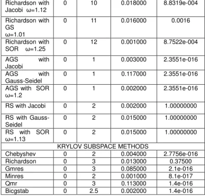
The results of the numerical experiments are presented in Tables 1 to 12. From Table 1 all the methods (the stationary methods, the accelerated schemes and the Krylov subspace acceleration methods) converged for the system considered. The Accelerated gradient scheme (AGS) converged faster than all the other methods (after just one or two iterations). The minimum and maximum optimal relaxation parameters for the stationary and acceleration schemes were 1.01 and 1.25 respectively. The number of iterations for both the acceleration schemes and Krylov subspace acceleration methods reduced drastically with the exception of that of Richardson with the stationary iterative methods. The speed indicates fast converges of the method even though it is relative, depending on the type of computer used. Each method has small relative residual which show that the approximation to the solution is stable and accurate.
Table 1 Banded System of size 4
ITERATIVE METHODS n = 4
Methods Flag Iteration Speed(sec) Relative Residual
Jacobi 0 10 0.109000 0.0020
Gauss-Seidel 0 7 0.063000 0.2500
SOR ω=1.11 0 5 0.015000 0.2500
ACCELERATION SCHEMES WITH ITERATIVE METHODS Chebyshev with
Jacobi
0 5 0.016000 2.7190e-004
Chebyshev with GS
0 6 0.031000 6.3746e-004
Chebyshev with SOR ω=1.22
0 6 0.023000 6.5033e-004
Richardson with Jacobi ω=1.12
0 10 0.018000 8.8319e-004
Richardson with GS ω=1.01
0 11 0.016000 0.0016
Richardson with SOR ω=1.25
0 12 0.001000 8.7522e-004
AGS with Jacobi
0 1 0.003000 2.3551e-016
AGS with Gauss-Seidel
0 1 0.117000 2.3551e-016
AGS with SOR ω=1.2
0 1 0.002000 2.3551e-016
RS with Jacobi 0 2 0.002000 1.00000000
RS with Gauss-Seidel
0 2 0.015000 1.00000000
RS with SOR ω=1.13
0 2 0.015000 1.00000000
KRYLOV SUBSPACE METHODS
Chebyshev 0 2 0.004000 2.7756e-016
Richardson 0 3 0.013000 0.37500
Gmres 0 3 0.085000 2.1e-016
Minres 0 2 0.001000 8.1e-017
Qmr 0 3 0.113000 1.4e-016
Bicgstab 0 2.5 0.002000 1.4e-016
From Table 2, the accelerated schemes and acceleration methods converged to a solution. For this type of problem, Residual smoothing (RS) converged faster than all the other methods. The minimum and maximum optimal relaxation parameters for the stationary and acceleration schemes are 0.9 and 1.25 respectively. Both the acceleration schemes and acceleration methods increased the rate of convergence of the stationary iterative methods with the exception of again the Richardson acceleration scheme. The computational time is relatively faster for each method. Each method had small relative residual which show that the solution is stable and accurate
Table 2 Banded System of size 6
ITERATIVE METHODS n = 6
Methods Flag Iteration Speed(sec) Relative Residual
Jacobi 0 18 0.027000
1.5033e-004 Gauss-Seidel 0 10 0.012000 0.2500 SOR ω=1.25 0 8 0.078000 0.2500 ACCELERATION SCHEMES WITH ITERATIVE METHODS Chebyshev with
Jacobi
0 5 0.022000
2.9888e-004 Chebyshev with
GS
0 7 0.006000
3.5396e-004 Chebyshev with
SOR ω=1.11
0 7 0.043000
4.5525e-004 Richardson with
Jacobi ω=0.9
0 20 0.072000 7.1319e-005 Richardson with
GS ω=1.11
0 19 0.043000 6.5047e-005 Richardson with
SOR ω=1.02
0 21 0.016000 8.0688e-005 AGS with Jacobi 0 6 0.109000
1.6249e-016 AGS with
Gauss-Seidel
0 6 0.010300
1.6249e-016 AGS with SOR
ω= 1.2
0 6 0.016000
1.7998e-420 016
RS with Gauss-Seidel
0 2 0.015000
1.7837e-016 RS with SOR
ω=1.13
0 2 0.005000
1.6794e-016 KRYLOV SUBSPACE METHODS
Chebyshev 0 2 0.015000
2.9199e-016
Richardson 0 6 0.016000 1.7e-016
Gmres 0 6 0.005000 1.6e-016
Minres 0 5 0.091000 4.5e-016
Qmr 0 6 0.048000 1.7e-016
Bicgstab 0 5 0.098000 5.7e-007
Table 3, indicates that all the methods (stationary, accelerated schemes and acceleration methods) converged to the approximate solution. Chebyshev acceleration and RS converges faster than the other methods. The minimum and maximum optimal relaxation parameters for the stationary iterative method and acceleration schemes are 0.9 and 1.12 respectively. The number of iteration for both the acceleration schemes and acceleration methods has decreased with the exception of Chebyshev with SOR and Richardson with the stationary iterative methods. The highest relative residual corresponds to Richardson acceleration scheme which does not improve the convergence of the stationary iterative methods.
Table 3 Banded System of size 9
ITERATIVE METHODS n = 9
Methods Flag Iteration Speed(sec) Relative Residual
Jacobi 0 24 0.050000
1.1630e-004 Gauss-Seidel 0 13 0.050000 0.25000 SOR ω=1.12 0 8 0.015000 0.25000
ACCELERATION SCHEMES WITH ITERATIVE METHODS Chebyshev with
Jacobi
0 5 0.021000
3.7993e-004 Chebyshev with
GS
0 9 0.017000
4.8422e-004 Chebyshev with
SOR ω=1.11
0 9 0.041000
9.5845e-004 Richardson with
Jacobi ω=0.9
0 26 0.021000 9.8621e-004 Richardson with
GS ω=1.11
0 25 0.015000 7.6202e-005 Richardson with
SOR w=1.11
0 28 0.015000 7.8968e-005 AGS with Jacobi 0 5 0.023000
2.5656e-016 AGS with
Gauss-Seidel
0 5 0.016000
2.5656e-016 AGS with SOR
ω= 0.9
0 5 0.015000
2.5656e-016 RS with Jacobi 0 2 0.031000
2.3024e-016 RS with
Gauss-Seidel
0 2 0.509000
1.1766e-016 RS with SOR
ω= 1.02
0 2 0.003000
8.8245e-017 KRYLOV SUBSPACE METHODS
Chebyshev 0 2 0.016000
1.2307e-016
Richardson 0 5 0.047000 2.7e-016
Gmres 0 5 0.005000 2.6e-016
Minres 0 5 0.005000 4.5e-016
Qmr 0 5 0.005000 2.7e-016
Bicgstab 0 4.5 0.004000 1.4e-016
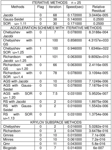
From Table 4, all the methods converged to an approximate solution except Chebyshev with Gauss-Seidel, Chebyshev with SOR and Richardson with Jacobi. RS and Chebyshev acceleration method converged faster than the remaining methods. The minimum and maximum optimal relaxation parameters for the stationary and acceleration schemes were 1.11 and 1.4 respectively. Richardson with SOR has converged but it does not improve stationary SOR method. The maxit for this problem is 1000 and still Chebyshev with Gauss-Seidel, Chebyshev with SOR and Richardson with Jacobi reached their maximum iteration with optimal relaxation parameters 1.25, 1.25 and 1.20 respectively.
Table 4 Banded System of size 25
ITERATIVE METHODS n = 25
Methods Flag Iteration Speed(sec) Relative Residual
Jacobi 0 68 0.172000 3.0440e-005
Gauss-Seidel 0 38 0.140000 0.2500 SOR ω= 1.11 0 30 0.171000 0.2500 ACCELERATION SCHEMES WITH ITERATIVE METHODS Chebyshev with
Jacobi
0 7 0.078000 8.3188e-004
Chebyshev with GS
1 100 0.858000 4.3157e+033
Chebyshev with SOR ω=1.25
1 100 0.946000 1.6346e+022
Richardson with Jacobi ω=1.25
1 101 0.063000 9.8092e+010
Richardson with GS ω=1.20
0 66 0.063000 2.4116e-005
Richardson with SOR ω=1.4
0 78 0.078000 3.1094e-005
AGS with Jacobi 0 10 0.015000 7.1249e-006 AGS with
Gauss-Seidel
0 10 0.078000 7.1876e-016
AGS with SOR ω= 1.20
0 7.5 0.031000 5.9520e-007
RS with Jacobi 0 2 0.015000 1.8975e-006 RS with
Gauss-Seidel
0 2 0.016000 1.5542e-006
RS with SOR ω=1.13
0 2 0.031000 1.3754e-006
KRYLOV SUBSPACE METHODS
Chebyshev 0 2 0.016000 5.0282e-016 Richardson 0 3 0.047000 3.6478e-016
Gmres 0 10 0.015000 7.1e-006
Minres 0 10 0.061000 7.2e-016
Qmr 0 11 0.043000 5.8e-016
Bicgstab 0 7 0.014000 6e-007
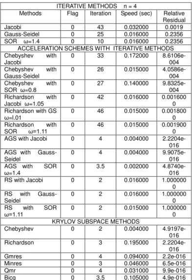
421 with the exception of that of RS scheme.
Table 5 SPD and Dense System of size 4
ITERATIVE METHODS n = 4
Methods Flag Iteration Speed (sec) Relative Residual
Jacobi 0 43 0.032000 0.0019
Gauss-Seidel 0 25 0.016000 0.2356
SOR ω=1.4 0 10 0.016000 0.2356 ACCELERATION SCHEMES WITH ITERATIVE METHODS Chebyshev with
Jacobi
0 33 0.172000 8.6106e-004 Chebyshev with
Gauss-Seidel
0 26 0.015000 4.0586e-004 Chebyshev with
SOR ω=0.8
0 27 0.140000 9.8325e-004 Richardson with
Jacobi ω=1.05
0 42 0.016000 0.001600 0 Richardson with GS
ω=l.01
0 46 0.015000 0.001800 0 Richardson with
SOR ω=1.11
0 46 0.015000 0.001900 0 AGS with Jacobi 0 4 0.004000
2.2204e-016 AGS with
Gauss-Seidel
0 4 0.004000
9.9075e-016 AGS with SOR
ω=1.4
0 3.5 0.002000 4.8740e-016 RS with Jacobi 0 2 0.016000 1.000000
0 RS with
Gauss-Seidel
0 2 0.016000 1.000000
0 RS with SOR
ω=1.11 0 2 0.015000 1.0000000
KRYLOV SUBSPACE METHODS
Chebyshev 0 2 0.004000
4.9197e-016
Richardson 0 3 0.195000
2.2204e-016
Gmres 0 4 0.094000 2.2e-016
Minres 0 3 0.046000 6.5e-016
Qmr 0 4 0.031000 9.9e-016
Bicg 0 3.5 0.105000 4.9e-016
Table 6 SPD System of size 6
ITERATIVE METHODS n = 6
Methods Flag Iteration Speed(sec) Relative Residual
Jacobi 0 34 0.082661
1.0859e-005 Gauss-Seidel 0 8 0.027405 2.1e-016 SOR ω=1.11 0 7 0.015000 0.0823
ACCELERATION SCHEMES WITH ITERATIVE METHODS Chebyshev with
Jacobi
0 6 0.035000
2.3993e-004 Chebyshev with
GS
0 6 0.015000
2.0110e-004 Chebyshev with
SOR ω=1.22
0 6 0.025000
2.6735e-004 Richardson with
Jacobi ω=0.60
0 16 0.067000
1.5153e-004 Richardson with
GS ω=0.90
0 13 0.003000
6.0218e-005 Richardson with
SOR ω=0.70
0 12 0.083000
5.2518e-005 AGS with Jacobi 0 6 0.007000
1.4413e-016 AGS with
Gauss-Seidel
0 6 0.005000
1.4413e-016
AGS with SOR ω= 1.25
0 6 0.005000
1.4413e-016 RS with Jacobi 0 2 0.009300 1.00000 RS with
Gauss-Seidel
0 2 0.007000 1.00000
RS with SOR ω=1.24
0 2 0.005000 1.00000
KRYLOV SUBSPACE METHODS
Chebyshev 0 2 0.005509 1.00000
Richardson 0 2 0.001440
1.0443e-016
Gmres 0 6 0.086621 5.2e-016
Minres 0 5 0.108678 1.3e-016
Qmr 0 6 0.079927 2.1e-016
Bicgstab 0 5.5 0.081156 1.3e-016
From Table 6, the methods converged to an approximate solution and Chebyshev with stationary have equal number of iteration (6). The RS scheme, Richardson and Chebyshev acceleration have equal and the fastest convergence. The minimum and maximum optimal relaxation parameters for the stationary and acceleration schemes are 0.6 and 1.25 respectively.
Table 7 SPD System of size 9 ITERATIVE METHODS n = 9
Methods Flag Iteration Speed(sec) Relative Residual
Jacobi 1 100 0.156000 1.5563e+02
3
Gauss-Seidel 0 6 0.047000 0.0825
SOR ω= 0.9 0 5 0.062000 0.0825 ACCELERATION SCHEMES WITH ITERATIVE METHODS Chebyshev with
Jacobi
0 8 0.094000 3.0967e-004
Chebyshev with GS
0 7 0.031000 9.3008e-004
Chebyshev with SOR ω=1.01
0 7 0.016000 0.0034
Richardson with Jacobi ω=1.25
1 101 0.067000 4.9336e+03 7 Richardson with
GS ω=1.01
1 101 0.047000 4.5069e+01 3 Richardson with
SOR ω=1.11
1 101 0.072100 8.0130e+01 2 AGS with Jacobi 0 5 0.031000 3.1592e-007 AGS with
Gauss-Seidel
0 5 0.015000 3.1592e-007
AGS with SOR ω= 0.9
0 5 0.016000 3.1592e-007
RS with Jacobi 0 2 0.031000 4.8449e-007 RS with
Gauss-Seidel
0 2 0.016000 4.3684e-007
RS with SOR ω=1.25
0 2 0.015000 3.8658e-007
KRYLOV SUBSPACE METHODS
Chebyshev 0 2 0.016000 2.7147e-016 Richardson 0 3 0.031000 3.0564e-008
Gmres 0 5 0.015000 3.2e-007
Minres 0 4 0.124000 3.2e-007
Qmr 0 5 0.124000 3.2e-007
Bicgstab 0 3.5 0.358000 2.4e-008
422 convergence. The minimum and maximum optimal relaxation
parameters for the stationary and acceleration schemes are 0.9 and 1.25 respectively.
Table 8 SPD System of size 25
ITERATIVE METHODS n = 25
Methods Flag Iteration Speed(sec) Relative Residual
Jacobi 0 95 0.952000
1.0182e-004
Gauss-Seidel 0 7 0.091000 0.0250
SOR ω= 0.9 0 6 0.063000 0.0250 ACCELERATION SCHEMES WITH ITERATIVE METHODS Chebyshev with
Jacobi
0 5 0.093000
1.2176e-004 Chebyshev with
GS
0 5 0.063000
1.0908e-004 Chebyshev with
SOR ω=0.9
0 4 0.031000
9.9137e-004 Richardson with
Jacobi w=0.6
0 8 0.054000
6.0392e-005 Richardson with
GS ω=0.6
0 8 0.013000
7.7639e-005 Richardson with
SOR ω=0.6
0 55 0.029000
9.5900e-005 AGS with Jacobi 0 4 0.088000
5.6974e-007 AGS with
Gauss-Seidel
0 4 0.045000
5.6974e-007 AGS with SOR
w= 0.6
0 4 0.018000
5.6974e-007 RS with Jacobi 0 2 0.046000 1.000000 RS with
Gauss-Seidel
0 2 0.032000 1.000000
RS with SOR ω=1.23
0 2 0.031000
8.5985e-007 KRYLOV SUBSPACE METHODS
Chebyshev 0 2 0.016000
6.5446e-017
Richardson 0 2 0.047000
1.0895e-007
Gmres 0 4 0.016000 5.7e-007
Minres 0 3 0.078000 5.7e-007
Qmr 0 4 0.016000 5.7e-007
Bicgstab 0 2.5 0.094000 4.6e-008
From Table 8, all the methods (stationary, accelerated schemes and acceleration methods) converged to an approximate solution. The RS scheme, Chebyshev and Richardson acceleration methods have the fastest convergence in terms of number of iterations. Even though Richardson with Gauss-Seidel and Richardson with SOR converged to an approximation solutions but they did not improve the convergence of the stationary iterative methods. The minimum and maximum optimal relaxation parameters for the stationary and acceleration schemes are 0.6 and 1.23 respectively
Table 9 Tridiagonal System of size 4
ITERATIVE METHODS n = 4
Methods Flag Iteration Speed(sec) Relative Residual
Jacobi 0 12 0.062000
1.8743e-004
Gauss-Seidel 0 7 0.015000 0.2000
SOR ω=1.12 0 5 0.016000 0.2000 ACCELERATION SCHEMES WITH ITERATIVE METHODS
Chebyshev with Jacobi
0 6 0.045000
4.1604e-004 Chebyshev with
GS
0 5 0.018000
7.1476e-004 Chebyshev with
SOR ω=1.3
0 0 0.009000
8.1091e-004 Richardson with
Jacobi ω=1.01
0 13 0.015000
1.2502e-004 Richardson with
GS ω=1.01
0 14 0.002000
6.0055e-005 Richardson with
SOR ω=1.05
0 12 0.016000
9.0377e-005 AGS with Jacobi 0 3.5 0.004000
1.9707e-016 AGS with
Gauss-Seidel
0 3.5 0.003000 1.9707e-016 AGS with SOR
ω= 1.12
0 3.5 0.003000 1.9707e-016 RS with Jacobi 0 2 0.094000 1.0000000 RS with
Gauss-Seidel
0 2 0.015000 1.0000000
RS with SOR ω=1.25
0 2 0.015000 1.0000000
ACCELERATION METHODS
Chebyshev 0 2 0.004000
2.6070e-016
Richardson 0 3 0.330000
9.8535e-017
Gmres 0 4 0.016000 9.9e-017
Minres 0 4 0.078000 0.00031
Qmr 0 4 0.078000 1.2e-016
Bicgstab 0 3.5 0.003000 2.9e-016
Table 9 indicates that the methods (stationary, accelerated schemes and acceleration methods) converged to an approximate solution. The RS scheme and Chebyshev acceleration method have the fastest convergence in terms of number of iterations. Richardson with stationary iterative methods converged to an approximate solution but did not improve the convergence of these stationary iterative methods.
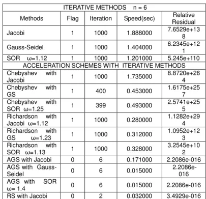
Table 10 Tridiagonal System of size 6
ITERATIVE METHODS n = 6
Methods Flag Iteration Speed(sec) Relative Residual
Jacobi 1 1000 1.888000 7.6529e+13
8
Gauss-Seidel 1 1000 1.404000 6.2345e+121
SOR ω=1.12 1 1000 1.201000 5.245e+110 ACCELERATION SCHEMES WITH ITERATIVE METHODS Chebyshev with
Jacobi 1 1000 1.735000
8.8720e+26 4 Chebyshev with
GS 1 400 0.453000
1.6175e+25 7 Chebyshev with
SOR ω=1.25 1 399 0.493000
2.5741e+25 5 Richardson with
Jacobi ω=1.12 1 1000 0.280000
1.1282e+29 4 Richardson with
GS ω=1.23 1 1000 0.312000
1.0952e+12 3 Richardson with
SOR ω=1.13 1 1000 0.328000
3.2545e+10 2 AGS with Jacobi 0 6 0.171000 2.2086e-016 AGS with
Gauss-Seidel 0 6 0.015000
2.2086e-016 AGS with SOR
ω= 1.4 0 6 0.015000 2.2086e-016
423 RS with
Gauss-Seidel 0 2 0.016000 1.5585e-015
RS with SOR
ω=1.13 0 2 0.014000 1.9939e-015
KRYLOV SUBSPACE METHODS
Chebyshev 0 2 0.003000 4.1012e-017
Richardson 0 2 0.008000 1.8069e-015
Gmres 0 6 0.160000 2.20e-016
Minres 0 6 0.088000 1.34e-.097
Qmr 0 6 0.347000 1.12e-015
Bicgstab 0 5.5 0.071000 3.90e-014
From Table 10, the methods converged to a solution except stationary iterative methods, Chebyshev with stationary iterative methods and Richardson with stationary iteration methods. The maxit was set to 1000 and still without converging to a solution. The minimum and maximum optimal relaxation parameters for the stationary and acceleration schemes are 1.12 and 1.4 respectively.
Table 11 Tridiagonal System of size 9
ITERATIVE METHODS n = 9
Methods Flag Iteration Speed(sec) Relative Residual
Jacobi 0 28 0.010000
2.1129e-005 Gauss-Seidel 0 16 0.010000 0.250000 SOR ω=1.12 0 11 0.025000 0.250000
ACCELERATION SCHEMES WITH ITERATIVE METHODS
Chebyshev with Jacobi
0 17 0.045000
6.0578e-004 Chebyshev with
GS
0 12 0.030000
8.7898e-004 Chebyshev with
SOR ω=0.60
0 10 0.050000
5.0506e-004 Richardson with
Jacobi ω=1.12
0 29 0.042000
1.3590e-005 Richardson with
GS ω=1.0
1 101 0.030000 5.2242e+0 08 Richardson with
SOR ω=1.20
1 101 0.040000 5.4020e+0 16 AGS with Jacobi 0 6 0.005000
4.6060e-016 AGS with
Gauss-Seidel
0 6 0.010000
4.6060e-016 AGS with SOR
ω= 0.9
0 6 0.005000
4.6060e-016 RS with Jacobi 0 2 0.006000
2.2480e-016 RS with
Gauss-Seidel
0 2 0.005000
4.8115e-016 RS with SOR
ω=1.13
0 2 0.005000
5.8376e-016 KRYLOV SUBSPACE METHODS
Chebyshev 0 2 0.000082 1.00000
Richardson 0 3 0.005000
1.1305e-016
Gmres 0 6 0.132780 7.5e-016
Minres 0 9 0.002641 1.8e-005
Qmr 0 6 0.002641 9.3e-016
Bicgstab 0 5.5 0.093143 1.6e-016
From Table 11, all the methods converged to an approximate solution with the exception of Richardson with Gauss-Seidel and Richardson with SOR and can be observed their relative residuals. The RS scheme and Chebyshev acceleration methods have the fastest convergence in terms of number of iterations. The minimum and maximum optimal relaxation
parameters for the stationary and acceleration schemes are 0.6 and 1.2 respectively.
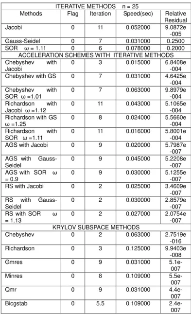
Table 12 Tridiagonal System of size 25
ITERATIVE METHODS n = 25
Methods Flag Iteration Speed(sec) Relative Residual
Jacobi 0 11 0.052000 9.0872e
-005
Gauss-Seidel 0 7 0.031000 0.2500
SOR ω = 1.11 0 6 0.078000 0.2000 ACCELERATION SCHEMES WITH ITERATIVE METHODS Chebyshev with
Jacobi
0 3 0.015000 6.8408e
-004 Chebyshev with GS 0 7 0.031000 4.6425e
-004 Chebyshev with
SOR ω =1.01
0 7 0.063000 9.8979e
-004 Richardson with
Jacobi ω =1.12
0 11 0.043000 5.1065e
-004 Richardson with GS
ω =1.25
0 8 0.024000 5.5660e
-004 Richardson with
SOR ω =1.11
0 11 0.016000 5.8001e
-004 AGS with Jacobi 0 9 0.020000 5.7987e
-007 AGS with
Gauss-Seidel
0 9 0.045000 5.2208e
-007 AGS with SOR ω
= 0.9
0 9 0.030000 5.1255e
-007 RS with Jacobi 0 2 0.025000 3.4609e
-007 RS with
Gauss-Seidel
0 2 0.030000 2.8579e
-007 RS with SOR ω
= 1.13
0 2 0.027000 2.0754e
-007 KRYLOV SUBSPACE METHODS
Chebyshev 0 2 0.063000 2.7519e
-016
Richardson 0 3 0.125000 9.9403e
-008
Gmres 0 9 0.031000
5.1e-007
Minres 0 8 0.109000
5.5e-007
Qmr 0 9 0.031000
4.4e-007
Bicgstab 0 5.5 0.109000
2.4e-007
From Table 12, all the methods (stationary iterative methods, the accelerated schemes and acceleration methods converged to an approximate solution. For this type of problem RS and Chebyshev acceleration methods converged faster than all the other methods in terms of number of iteration. The minimum and maximum optimal relaxation parameters for the stationary iterative methods and acceleration schemes are 0.9 and 1.25 respectively. For this problem only the acceleration methods, RS scheme and Chebyshev with Jacobi improved the convergence of the stationary iterative methods.
Conclusions
424 These were more so with Richardson with Gauss-Seidel,
Richardson with SOR, Chebyshev with Gauss-Seidel and Chebyshev with SOR. The iterative schemes were applied to Banded system, Tridiagonal systems and SPD system with varying dimensions. The Krylov subspace methods: GMRES, QMR, MINRES and BiCGSTAB converged to an approximate solutions less than or equal to the dimension of the coefficient matrix for each identified systems of linear equations. Again, Chebyshev and Richardson acceleration methods were the fastest convergence methods in terms of number of iterations. Again, Residual smoothing and the accelerated gradient schemes should be used for large and sparse systems of linear equations. The acceleration processes were very efficient when solving large and sparse systems of linear equation and therefore useful especially for systems resulting from the solution of partial differential equations.
REFERENCES
[1] Fink, K.D and Mathews, J.H. (2004). Numerical Methods Using Matlab 4th Edition. Person Education Inc, Upper Saddle River. New Jessey
[2] Iqbal J, Arif M, Ayaz M, (2013). Preconditioned Iterative methods for Linear Systems. Life Science Journal 10(3s): 467-470
[3] Santos, R. and Linhares (1986). Convergence of Chebyshev Semi-Iterative methods.Journal of Applied Mathematics 16(59-68).North-Holland.
[4] Wrigley, H.E. (1963). Accelerating the Jacobi method for solving simultaneous equations When the eigenvalue of iterative methods are complex.www.ams.org/mcom/1984-42-166/S0025-5718-1984-0736453-8
[5] Varga, R.S. (1962). Matrix Iterative Analysis. Prentice-Hall, Englewood Cliffs, N.J
[6] Hadjidimos A, (1978). Accelerated Overrelaxation Method. Mathematics of Computation. 32(141): 149-157
[7] Brezinski, C. (1996).Variations of Richardson’s methods and acceleration. Mathematics Subject Classification. 33-44
[8] Young D.M, Iterative Solution of Large Linear Systems, Academic Press, New York, NY, USA, 1971.
[9] Bai, Y. Xiao, Y. and Ma, W. (2013). The Preconditioned SOR Iterative methods for Positive Definite Matrices. A journal of Applied Mathematics.
www.hindawi.com/journals/jam/2013/732834.pdf
[10] Gutknecht, M.H. and Rolin, S. (2002) . Chebyshev
iterative Revisited. Parallel Computing. 26 (263 – 283).
[11] Duan, L. and Zheng, B. (2008). Chebyshev polynomial acceleration of SOR solving the rank of Deficient linear system.. Department of Mathematics, Lanzhou University
a. Lanzhou 730000, PR China. 1-16
[12] Kelley, C.T. (1995). Iterative methods for linear and Nonlinear Equations. Society for Industrial and Applied
Mathematics. http://www4.ncsu.edu/~ctk/fr16_book.pdf